Article

A Prediction Model of Water In Situ Data Change under the Influence of Environmental Variables in Remote Sensing Validation

1
Aerospace Information Research Institute, Chinese Academy of Sciences, Beijing 100101, China
2
School of Electronic, Electrical and Communication Engineering, University of Chinese Academy of Sciences, Beijing 100049, China
*
Author to whom correspondence should be addressed.
Remote Sens. 2021, 13(1), 70; https://doi.org/10.3390/rs13010070
Submission received: 27 November 2020 / Revised: 21 December 2020 / Accepted: 23 December 2020 / Published: 27 December 2020
(This article belongs to the Special Issue Earth Observations in Asia-Oceania)

Abstract

:
Validation is an essential process to evaluate the quality of waterbody remote sensing products, and the reliability and effective application of the in situ data of waterbody parameters are an important part of validation. Based on the in situ data of chlorophyll-a (Chl-a), total suspended solids (TSS) and other environmental variables (EVs) measured at the fixed station in Taihu Lake, we attempt to develop a prediction model to determine whether the in situ measurement has enough representativeness for validating waterbody remote sensing products. Key EVs that affect the changes of Chl-a and TSS are firstly identified by using correlation analysis, which participate in modeling as variables. In addition, three multi-parameter modeling approaches are selected to simulate the daily changes of Chl-a and TSS under different EVs configurations. The results indicate that the highest prediction accuracy can be achieved through the generalized regression neural network (GRNN) based model. In the all-valid dataset, the testing absolute average relative errors (AEs) of GRNN-based Chl-a and TSS prediction model are 11.4% and 11.3%, respectively, and in the sunny-day dataset, the testing AEs are 8.6% and 8.2%, respectively. Meanwhile, the application example proves that the prediction model in this paper can be effectively used to screen the in situ data and determine the time window for satellite-ground data matching.

1. Introduction

Affected by anthropogenic activities, especially in industrial areas, water pollution and other water environmental issues have become increasingly prominent, attracting more and more attention [1]. Conventional methods for water quality evaluation depend on costly, time and labor-intensive on-site sampling and data collection [2]. Satellite remote sensing can provide large-scale and long-term observational data, which provide the possibility to dynamically measure and monitor water environment. Chlorophyll-a concentration (Chl-a) and total suspended solids concentration (TSS) generated from remote sensing satellite data are two typical remote sensing products (RSPs), among which Chl-a is an important indicator for red tide monitoring and water eutrophication monitoring [3,4], and TSS is related to water transparency, total primary production, and fluxes of heavy metals and micro-pollutants [1,5]. Furthermore, these two RSPs are the basis of other more advanced products such as net primary productivity (NPP) and water quality [6]. However, the quality of RSPs has been questioned by many researchers, which also restricts their development and application [7]. Therefore, it is very important to evaluate and verify the quality and accuracy of RSPs, which is also called validation. The validation in remote sensing refers to analyzing the accuracy and uncertainty of RSPs by using relative truth values that can represent the characteristics of ground targets [8,9].
Over the past few decades, researchers all over the world have carried out much related work in remote sensing validation. The National Aeronautics and Space Administration (NASA) proposed the Earth Observation System (EOS) project after launching moderate resolution imaging spectroradiometer (MODIS) sensors, which firstly developed remote sensing validation systematically and laid the foundation for validation of RSPs [10]. In the early twentieth century, European Space Agency (ESA) launched the Validation of Land European Remote Sensing Instruments (VALERI) program, which acquired multi-scale and long-term earth observation data within Europe. These data have been widely used in the validation of terrestrial RSPs of MODIS, medium resolution imaging spectrometer (MERIS), and other sensors [11]. Based on these projects, the Committee Earth Observation Satellite (CEOS) set up the Land Product Validation (LPV) working group. The LPV group creatively raised cross-validation between RSPs of different sensors, which plays a guiding role in the global validation work [12,13]. In addition, there are many research institutions in different countries that have carried out validation-related work and made outstanding contributions, such as Canada’s Boreal Ecosystem Research and Monitoring Sites (BERMS), the Large Scale Biosphere-Atmosphere Experiment in Amazonia (LBA), etc. [14,15]. From 2007 to 2010, a number of Chinese institutions jointly carried out the Watershed Airborne Telemetry Experimental Research (WATER) project in Heihe river basin, laying the basis for the development of RSPs’ validation in China [16,17].
The validation of waterbody RSPs usually adopts direct-validation, that is, the product data retrieved by satellites are directly compared with the in situ data [18], and the accuracy of in situ data is of significance [9]. Not only the reliability of validation, but also the in situ data accuracy determines the model’s calibration reliability to retrieve the optically active components (OACs). In recent years, to ensure the accuracy of in situ data, many researchers have carried out a lot of work in in situ data measurement, such as designing sampling schemes and deploying wireless sensor networks to obtain long-term observation data, etc. [19,20,21]. However, most researches focus on land surface. Different from land, the high cost of equipment and complex water environment make it very difficult to deploy wireless sensor observation networks on water surface [22]. Usually, sampling observation with boat by experimenters is still the most commonly used method to obtain in situ data of waterbodies [23,24].
Generally, validation of RSPs requires real-time synchronized observing of ground data [25]. In fact, ground measurement takes more time, while satellite transit is almost instantaneous. Moreover, the number of samples should not be less than the necessary minimum sample size for statistical reliability [25], and the representativeness of the in situ data will be better with more samples measured in the experimental area. According to our experimental experience, waterbody sampling and measuring are extremely time-consuming. It usually takes about 5 min to measure waterbody parameters of one sampling site, and the sailing of the experimental ship between different sites also kills a lot of time. Therefore, the measurements of multiple sampling sites cannot be all completed in a short time before and after the satellite transits. Usually, to obtain high-quality in situ data at each sampling site, the measurements of waterbody parameters should be performed under clear skies, with no wind or low winds [26]. However, due to the long observing time, environmental factors such as temperature, wind speed, wind direction, humidity, and atmospheric pressure keep changing, leading to variations of waterbody parameters even at the same sampling site.
The fluctuation of in situ waterbody parameters during the measuring time will bring errors to validation. How to effectively use the in situ data within the measurement time is also an important issue in validation. In the current work of waterbody RSPs validation, the error is mainly controlled by limiting the spatiotemporal match-up window of satellite–ground data. Using the resolution of a 3 × 3 pixel box and ±3 h as the match-up window, Sun et al. validated Chl-a products of MODIS Aqua by using the in situ data collected in the Yellow Sea and the East China Sea in the spring and autumn of 2003 [27]. Zhao et al. verified the remote sensing reflectance and Chl-a products of the sea-viewing wide field-of-view sensor (SeaWiFS), MODIS, and MERIS in the South China Sea with the strict spatiotemporal match-up data [28]. The results showed that when the match-up criteria were relaxed, the assessment results degraded systematically. Bailey et al. also clearly indicated that the time lag between the satellite and in situ data should not exceed ±3 h [25]. Palmer assumed that the Chl-a of ±3 h would not change significantly. Based on this, the long-term observing in situ data of Lake Balaton was used to validate MERIS satellite data, demonstrating that MERIS satellite data is effective in retrieving Chl-a accurately [29]. In addition, some validation activities for algorithm models also limit sampling within a certain time window, such as the validation of Kd(490) and Chl-a estimation algorithm, to ensure that the time interval between satellite and in situ data will not be too long [30,31]. Although the spatiotemporal match-up window reduces the error of waterbody RSPs validation to some extent, these empirical methods do not solve the reliability problem of in situ data.
In order to cope with the uncertainty in validation caused by the changes of in situ data during the sampling period, we attempt to develop a prediction model of Chl-a and TSS based on the in situ measurement for determining whether the in situ measurement has enough representativeness or not for validating waterbody RSPs. We investigated the influences of complex environmental factors on the Chl-a and TSS variations at the temporal scale, tried to use numerical simulation methods to simulate the temporal pattern of Chl-a and TSS changes, and established a predictive analysis model. This prediction model is used to evaluate the reliability of in situ waterbody parameters and to provide a reference for the selection of in situ data and the matching of satellite–ground data.

2. Data and Preprocessing

2.1. Experimental Area and Instruments

Taihu Lake is a typical large-scale eutrophic shallow lake in China (30°55′040″–31°33′58″N, 119°52′32″–120°36′10″E). It has a mean depth of 1.9 m and Chl-a and TSS in the lake have obvious seasonal variations [32,33,34]. This obvious seasonal change has led to a very wide range of waterbody parameters and also contributed to the generalization of research results. The experimental measuring instruments are placed near the water quality monitoring platform (31.216667°N, 120.283333°E) of Taihu Lake, and the location and instruments are shown in Figure 1. The layout of these instruments strictly abides by the corresponding national standard. The waterbody spectrometer is installed on the platform, the buoy system equipped with a multi-variables water quality meter, and a portable weather station is fixed beside the platform, and the multi-variables water quality meter is set to collect data from a 30 cm water depth. These instruments have been calibrated in the laboratory of Ocean University of China before installation to ensure their measurement accuracy. At the same time, these instruments are recalibrated every three months to ensure the stability of long-term measurements. In addition, all the observation data will be uploaded to the server every day and be checked by professionals.
All of the above instruments adopt automatic observation mode, in which the waterbody spectrometer observes every 30 min from 10:00 to 15:00 of local time and takes a photo reflecting the weather conditions. The multiple parameter water quality meter and the portable weather station observe every 30 min throughout the day, and each observation is the average of five readings. The measured data includes WT (water temperature, °C), SpC (specific conductivity, μS/cm), Cond (conductivity, μS/cm), Sal (salinity, ppm), Chl-a (μg/L), PC (phycocyanin, μg/L), FDOM (fluorescent dissolved organic matter, ppb QSE), TSS (mg/L), AWD (average wind direction, °), AWS (average wind speed, m/s), AT (air temperature, °C), AH (air humidity, %), and AP (atmospheric pressure, hpa).

2.2. Data Preprocessing

From May 2019 to May 2020, a total of 3740 observed data were obtained between 10:00 a.m. and 15:00 p.m., local time. Data preprocessing was completed in three steps.
(1)
Firstly, the original data were screened to eliminate the invalid data caused by instrument calibration, damage, and maintenance, such as the data with Chl-a ≤0 and TSS equal to −9999. A total of 2166 effective measured data were collected after elimination.
(2)
Secondly, considering that some EVs (such as Sal, PC, FDOM, AWD, and AP) do not satisfy the normal distribution, we introduced the adjusted boxplot to eliminate the outliers, which take into account the medcouple (MC), a robust measure of skewness for a skewed distribution [35]. These outliers may be caused by other uncontrollable factors such as occlusion of floating objects or fishing boats passing by. After processing, a total of 1692 available Chl-a data were collected, accounting for 78.1% of the effective measured data. Because there are more outliers in TSS data during measurement, the available TSS data amounted to 1627, accounting for 75.1%. The available Chl-a data and TSS data both form the all-valid dataset. According to statistics, the range of Chl-a in all-valid dataset is between 0.46 μg/L and 8.19 μg/L, and the range of TSS is between 5.8 mg/L and 80.1 mg/L.
(3)
Finally, the data of sunny days were selected based on the photos taken by the waterbody spectrometer. A total of 403 Chl-a data and 382 TSS data were collected, forming the sunny-day dataset. According to statistics, Chl-a in the sunny-day dataset ranges from 0.62 μg/L to 6.15 μg/L, and TSS ranges from 16.3 mg/L to 80.0 mg/L.

3. Method

3.1. Correlation Analysis

The changes of Chl-a and TSS are closely related to environmental variables (EVs). In this paper, the Spearman rank correlation coefficient ( ρ , rho) was used to examine relationships among Chl-a, TSS, and EVs. The expression of ρ is shown in Formula (1), where d i represent the difference between the ranks of corresponding two variables, and n is the number of observations. The two variables are independent of each other when ρ equals to 0, and ρ > 0 indicates the variables are positively correlated, while ρ < 0 means negatively correlated. Usually, | ρ | ≤ 0.2 means very weak or negligible correlation, and | ρ | > 0.2 means that the correlation between two variables need to be considered [36].
ρ = 1 6   d i 2 n ( n 2 1 )

3.2. Multi-Variables Modeling Method

To comprehensively analyze the effects of various EVs on Chl-a and TSS, three multi-variables modeling methods including multiple linear regression (MLR), back propagation neural network (BPNN), and generalized regression neural network (GRNN) were used as modeling functions in this paper. Among them, MLR is a statistical technique that uses the optimal linear combination of several explanatory variables to predict the outcome of a dependent variable [37]. MLR is simple and efficient, which can effectively use the information of multiple related variables to achieve high prediction accuracy. However, MLR requires a high correlation between independent variables and dependent variables, and its performance is not as good as BPNN in nonlinear problems. BPNN is one of the basic neural networks, it has excellent performance in dealing with multivariate and nonlinear relationships. Up to now, BPNN has been widely used in the retrieval of remote sensing parameters [38,39,40,41]. However, two shortcomings of BPNN restrict its application: (1) Convergence is slow during training, and (2) BPNN is too sensitive to the initial network weights, and different initial weights help the model converge to different local minimums [42]. Compared to BPNN, GRNN, which is a special radial basis neural network, has superior positioning ability and convergence speed, and can converge to the global minimum [42]. Many studies in the remote sensing field can be accomplished with GRNN, such as the estimation of soil moisture, leaf area index, and mapping particulate matter (PM2.5, particulate matters with aerodynamic diameters less than 2.5 μm) distribution [43,44,45]. However, one of the disadvantages of GRNN is the growth of the hidden layer size, which would make it computationally expensive [46]. All the methods have its own advantages and disadvantages; we carried out modeling with three methods and selected the best models to predict the daily changes of in situ Chl-a and TSS.

3.3. Multi-Parameters Forecasting Model

In order to assess the stability of the in situ Chl-a and TSS, we tried to explore the changing rules of Chl-a and TSS on a daily time scale. In fact, the changes of EVs are continuous, and the waterbody parameters also show the characteristic of continuous changes under the influence of EVs. Therefore, in this paper, the in situ data measured every 30 min from 10:00 to 15:00 was used to train and fit the daily change patterns of Chl-a and TSS, and models were established to predict their changes. Chl-a and TSS predicted by the models can be expressed by following equations.
Chl-a tm = f ( Chl-a t 0 , Δ t , x 1 t , x 2 t , , x mt )
TSS tm = f ( TSS t 0 , Δ t , y 1 t , y 2 t , , y nt )
Δ t = t t 0 ,   and 5 h Δ t 5   h
where t0 represents the observation moment between 10:00 to 15:00, and t represents the moment needs to be predicted in the same time range, but it can not be equal to t0. Δ t represents the interval between the observation time and prediction time. Chl-a t 0 and TSS t 0 are the in situ Chl-a and TSS at the observation time t0, while Chl-a tm and TSS tm are the predicted Chl-a and TSS at other time t. x 1 t , x 2 t , , x mt , y 1 t , y 2 t , , y nt are the EVs at time t that cause changes in Chl-a and TSS, respectively, m and n are the number of variables, and f represents a function, which can be MLR, BPNN, or GRNN.
On this basis, we first calculated the time interval Δ t between any two observation moments in the same day, that are t and t0. Then many combinations of two different observation times of the same day were used for forming the data vectors [ Chl-a t 0 , Δ t , x 1 t , x 2 t , , x mt , Chl-a tr ] and [ TSS t 0 , Δ t , y 1 t , y 2 t , , y nt , TSS tr ] , where Chl-a tr and TSS tr are the measured Chl-a and TSS at time t.

3.4. Evaluation Index of Model Accuracy

In addition, coefficient of determination ( R 2 ), root mean square error (RMSE) and absolute average relative error (AE) are chosen as the indicators to evaluate the accuracy of the models. The calculation methods are as shown in the following formulas.
R 2 =   ( X m X m ¯ ) ( X r X r ¯ )   ( X m X m ¯ ) 2   ( X r X r ¯ ) 2
RMSE = i = 1 N ( X m ( i ) X r ( i ) ) 2 N
AE = | X m X r | ¯ | X r | ¯
where N is the number of data, X m is the predicted results, and X r is the in situ data.

3.5. Impact Factor Screening

In order to describe the relationship between Chl-a, TSS, and EVs, we firstly analyzed the correlation of Chl-a, TSS, and other variables, and selected the variables with higher correlations. Secondly, in order to reduce the redundancy of modeling variables and avoid the problem of multiple-collinearity, we conducted correlation analysis among the selected EVs. If the ρ of two variables is greater than 0.5, they cannot both be selected as modeling variables, and only the variables that have higher ρ with Chl-a or TSS can be selected.

4. Results

4.1. Correlation Analysis

4.1.1. Variable Correlation Analysis

The correlation between Chl-a, TSS, and other EVs were analyzed, and ρ was used to characterize the correlation, as shown in Table 1. Taking | ρ | > 0.2 as the criterion, WT, SpC, Cond, Sal, FDOM, AWS, AT, and AP are correlated with Chl-a, and WT has the highest ρ . The absolute value of ρ between the remaining variables and Chl-a are less than 0.2, which are weak correlation factors. Furthermore, WT, Cond, AWS, and AT are positively correlated with Chl-a, while SpC, Sal, FDOM, and AP are negatively correlated with Chl-a. According to Table 1, the EVs correlated with TSS are WT, Cond, FDOM, AWD, AWS, and AT. Among them, AWD and AWS are positively correlated with TSS, while WT, Cond, FDOM, and AT are negatively correlated with TSS. Besides them, the | ρ | of other variables and TSS are less than 0.2, which are not significant factors.

4.1.2. Correlation Analysis Among EVs

To reduce the redundancy of modeling variables, correlation analysis using ρ was performed among WT, SpC, Cond, Sal, FDOM, AWD, AWS, AT, and AP that correlated with Chl-a and TSS. From Table 2 we can see, WT, Cond, and AT are closely correlated with each other, and ρ values are all greater than 0.8. SpC is closely correlated with Sal, and their ρ equals to 0.98. AWD and AWS are weakly correlated with other EVs, all the ρ values are less than 0.2.

4.1.3. Environment Variable Filtering

According to the results of correlation analysis, the ρ between WT and Chl-a is the highest, which is 0.49. Actually, WT is related to light intensity and closely related to the growth of phytoplankton, so WT is one of the indispensable variables that affects changes of Chl-a [47]. Although AT and Cond are also correlated with Chl-a, these two variables have a strong correlation with WT, respectively, so AT and Cond are discarded during model construction in this paper. In addition, both AP and AWS are correlated with Chl-a, ρ is −0.43 and 0.33, respectively, and the ρ with other variables is less than 0.5, so both of them were selected as modeling variables. Finally, SpC is more closely correlated with Chl-a compared to Sal, ρ of which is −0.39 and −0.34, respectively, and the ρ between SpC and Sal is 0.98; therefore, we only chose SpC as one of modeling variables. FDOM is consisted of humic-like components, tryptophan-like components, autochthonous tyrosine-like components, etc. [47]. The main source of FDOM in the lake is from microbes and algae, and its distribution has high spatial heterogeneity in lakes [48]. Although FDOM is correlated with Chl-a, it was not considered as the input variable for the modeling due to its high spatial heterogeneity. In summary, WT, SpC, AWS, and AP were selected as the modeling variables to build the Chl-a prediction model.
For TSS, AWS has the highest correlation with TSS, the ρ equals to 0.37. The suspension of solid particles is inseparable from wind speed in the lake, especially in the shallow lake like Taihu, so AWS is an effective modeling variable. Secondly, the ρ between Cond and TSS, AWD, and TSS are −0.27 and 0.25, respectively. Additionally, Cond and AWD are weakly correlated with AWS, and ρ is only 0.03 and −0.02, respectively, so Cond and AWD can be used as modeling variables. WT and AT are correlated with TSS, but the correlation coefficients with the selected variable Cond are greater than 0.5, so they were excluded in this paper. Finally, considering the spatial heterogeneity, FDOM still did not participate in modeling. In summary, AWS, Cond, and AWD were selected as the modeling variables to build TSS prediction model.

4.2. Modeling Results in All-Valid Dataset

4.2.1. Model Results of Chl-a

In order to build the Chl-a prediction model, the selected WT, SpC, AWS, AP variables, and preprocessed Chl-a data were used to form data vectors according to the vector structure mentioned in 3.3, and the all-valid Chl-a dataset was built based on these data vectors. There are 1692 Chl-a records available after preprocessing, forming 15,113 data vectors in the dataset. Before modeling, we first counted the observation dates of all the data vectors, and then selected the data from the random 85% of the dates as the training dataset, and the remaining 15% as the testing dataset, to ensure that the testing dataset is perfectly separated from the training dataset. Both the training dataset and the testing dataset were used to build and verify the prediction models with MLR, BPNN, and GRNN method. The expression of the models and the accuracy evaluation results are shown in Table 3.
The accuracy evaluation results in Table 3 show that, except for the R 2 of MLR-based model are 0.78 and 0.72, respectively, which are lower than 0.8, R 2 of two neural network-based models are more than 0.8, the RMSE of three models are all less than 0.7, and all the AE are less than 20%. When comparing the accuracy of the three models, R 2 , RMSE, and AE in Table 3 all show that the model’s accuracy is improving gradually from MLR to BPNN and to GRNN. The most accurate of the three models is the GRNN-based prediction model; its modeling and testing AE are 8.2% and 11.4%, respectively. Considering the requirement of traditional RSPs validation issues, we assumed that AE less than 10% is the target accuracy of this paper. On this basis, the accuracy of the GRNN-based model is close to the target accuracy, which proves that the four environmental variables WT, SpC, AWS, and AP selected in Section 4.1 are very representative; the forecasting models based on them can predict the daily change of Chl-a well.
In addition, the coefficient of Chl-a t 0 is as high as 0.82 in MLR-based model, which can be attributed to two aspects. First, Chl-a t 0 and Chl-a t are of the same value ranges, so the coefficient of Chl-a t 0 is closer to 1, while the coefficients of other variables, such as WT, SpC, and AWS, are smaller. Second, larger coefficient shows that Chl-a t 0 has a greater contribution to the model, the measured Chl-a at time t0 is critical to predicting the changes of Chl-a at other moments of the same day.

4.2.2. Modeling Results of TSS

Regarding TSS, the selected AWS, Cond, AWD variables, and the 1627 pieces of available TSS were used to build data vectors according to the vector structure in 3.3. A total of 11,943 data vectors were collected to form the all-valid TSS dataset. Similarly, the data measured in the random 85% of the dates (10,078) were used for modeling, and the remaining 15% (1865) were used to test the accuracy of the models. The evaluation indexes in 3.4 were used to measure the accuracy of models, and the results are shown in Table 4.
In Table 4, the accuracy evaluation results of three TSS models show that all R 2 are higher than 0.85, RMSE are less than 9, AE are lower than 20%. The accuracy indicators prove that the method of multi-parameters forecasting model in this paper is suitable to TSS, and the three selected EVs, namely, Cond, AWS, and AWD are very representative. In addition, the equation coefficient of TSS t 0 in MLR model expression is up to 0.90, indicating that the dominant factor for the change of TSS at the same point is TSS t 0 . Similarly, the accuracy of BPNN-based model is higher than that of MLR-based, the accuracy of GRNN-based model is the highest, and AEs of GRNN-based model are 8.9% and 11.3%, respectively. According to the statistical results, the range of TSS in all-valid dataset is between 5.8 and 80.1 mg/L. For the TSS that varies within a large threshold range, a model with AE close to 10% is sufficient to predict the daily change of TSS.

4.3. Modeling Results in Sunny-Day Dataset

In Section 4.2, all-valid data with a one-year observation time span was used for modeling and testing, covering variables measured under various complex weather conditions. The models based on these data have good performance, which proves that the multi-parameter forecasting model method in this paper is effective. In fact, in order to obtain sufficient in situ data and high-quality satellite images, the validation experiments of waterbody RSPs usually choose sunny days with clear sky or few clouds. Therefore, the sunny-day dataset collected in Section 2.2 were used to conduct further analysis, and the results are as follows.

4.3.1. Environment Variable Filtering

Similarly, we carried out correlation analysis on the sunny-day data in order to select the EVs that have good correlation with Chl-a and TSS. The correlation analysis results are shown in Table 5. Taking | ρ | > 0.2 as the criterion, Table 5 shows that the variables correlated with Chl-a are WT, PC, AWS, AT, and AP, and the variables correlated with TSS are WT, Cond, PC, FDOM, AWS, and AT. Among them, PC is a pigment–protein complex from the light-harvesting phycobiliprotein family and is found in cyanobacteria, Rhodophyceae, and Cryptophyceae. Like FDOM, PC is related to the distribution of phytoplankton, and has high spatial heterogeneity in Taihu Lake [49]. Therefore, both of FDOM and PC are not suitable to be selected as modeling variables. Correlation analysis was then conducted among WT, Cond, AWS, AT, and AP, and the correlation coefficients are shown in Table 6.
Comprehensively considering the correlation between Chl-a/TSS and EVs, and also the correlation among EVs, three variables, namely, AWS, AP, and AT were selected to participate in the construction of Chl-a prediction model, and AWS, AT, and Cond were selected as modeling variables to build TSS prediction model.

4.3.2. Modeling Results

After preprocessing, a total of 3499 data vectors were built based on 403 records of valid sunny-day Chl-a dataset. The data vectors from the separated 85% of the dates, namely 2963 records of data, were randomly selected as the training set, and the remaining 536 records of data as the testing set. A total of 3246 data vectors were formed using 382 records of valid TSS data in the sunny-day dataset. Similarly, the data of the 85% dates were selected as modeling set, and the remaining 497 pieces were used as testing set. The accuracy evaluation results of Chl-a and TSS models are shown in Figure 2 and Figure 3, respectively.
From Figure 2, we can see the testing RMSE for MLR, BPNN, and GRNN-based Chl-a prediction models by using sunny-day Chl-a data are 0.51, 0.37 and 0.29, while the RMSE listed in Table 3 for three prediction models constructed using all-valid Chl-a data are 0.63, 0.54, and 0.41. The testing AEs for three Chl-a prediction models by using sunny-day data are 17.8%, 13.4%, and 8.6%, while the AEs listed in Table 3 for three prediction models constructed using all-valid Chl-a data are 18.9%, 15.6%, and 11.4%. So we can say that the performance of the MLR, BPNN, and GRNN-based models built with the sunny-day dataset are much better than those models base on the all-valid dataset. The same conclusion is satisfied with TSS prediction models.
GRNN-based forecasting models for Chl-a and TSS have the highest accuracy no matter what kinds of data are used to construct them. From Figure 2 and Figure 3, it can be seen that the in situ data and prediction data by using a GRNN-based model have more tight positive correlation than other models. RMSE of GRNN-based prediction models of Chl-a and TSS are 0.29 and 4.85, which is significantly lower than other models. In addition, the AEs of GRNN-based prediction models of Chl-a and TSS are only 8.6% and 8.2%; both are less than 10%, which can effectively predict the changes of Chl-a and TSS.
In addition, we performed statistical analysis on the residuals of the GRNN-based model built in the sunny-day dataset. The result shows that the mean values of the residuals of the GRNN-based Chl-a and TSS models were −0.0016 and −0.0131, respectively, both of which are close to zero, and the residuals of the two models basically satisfied the normal distribution, which proves that the models in this paper are reliable.4.4. Time Dependence of the Accuracy of GRNN-Based Prediction Model.
In order to evaluate the time dependence of the accuracy of GRNN-based prediction model, we divided the data vectors according to the standards of | Δ t | ≤ 1 h, 1 h < | Δ t | ≤ 2 h, 2 h < | Δ t | ≤ 3 h, 3 h < | Δ t | ≤ 4 h, and 4 h < | Δ t | ≤ 5 h, and preformed modeling analysis. The testing accuracy of the model is shown in Table 7, where Num. represents the amount of data.
It can be seen from the results in the table that for the all-valid and the sunny-day datasets, as | Δ t | increases, the values of the three accuracy indicators of R 2 , RMSE, and AE gradually increase, and the accuracy of the model gradually declines. When | Δ t | ≤ 1 h, the Chl-a and TSS prediction models built with two datasets all have the highest accuracy. When | Δ t | is between 1 and 3 h, the accuracy of the model basically meets our expectations and can accurately predict Chl-a and TSS. However, when | Δ t | is greater than 3 h, the accuracy of the model may not be sufficient to support effective prediction of Chl-a and TSS changes. It is worth noting that the amount of data used for modeling and testing is different when the values of | Δ t | are in different time ranges, which requires us to accumulate more data to further study the time dependence of the prediction model.

4.4. Model Prediction Results

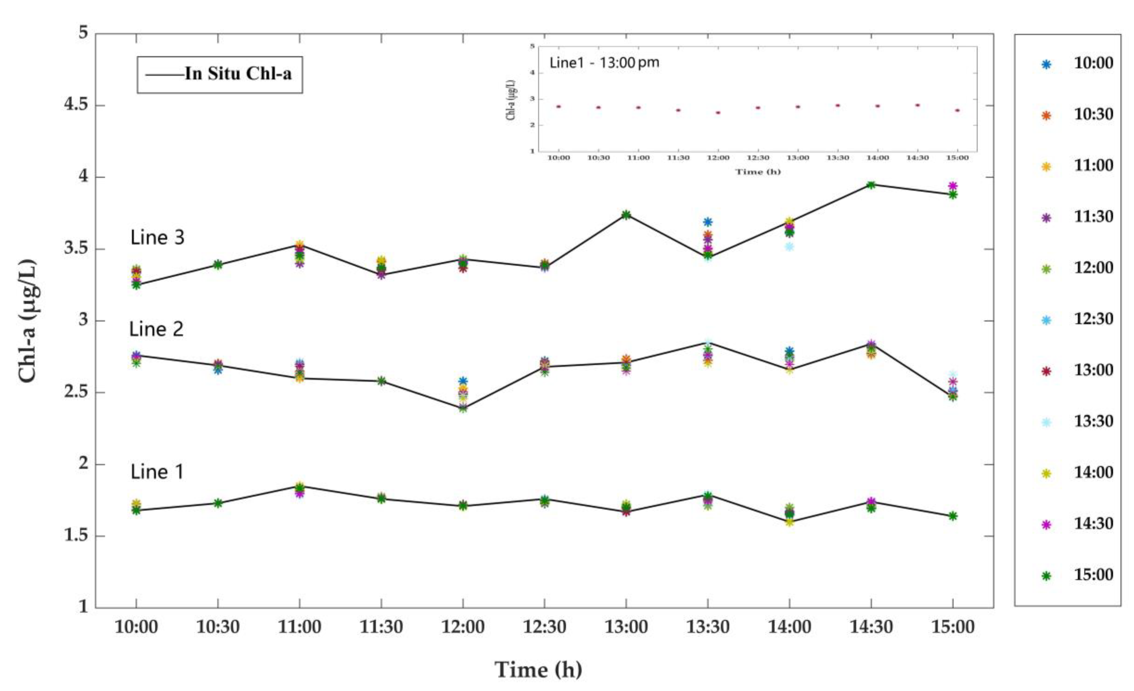
Figure 4 shows the prediction results of Chl-a using a GRNN-based model constructed under sunny weather conditions. In order to explore the applicability of this model in a different concentration range, the measured Chl-a around 1.5 (Line 1), 2.5 (Line 2), and 3.5 μg/L (Line 3) were selected as the baselines to predict the value in other moments. In this figure, in situ Chl-a are represented by black lines, and the predicted Chl-a are represented by colored dots. There are 11 observing moments between 10:00 and 15:00, the in situ Chl-a at each moment can be used as baseline to predict Chl-a at the other 10 moments. For example, if we want to predict the Chl-a at 11:00, we can take the Chl-a measured at 10:30 as the baseline, use the EVs at 11:00 as the input variables and set Δ t as 0.5 for the prediction model. Similarly, the in situ Chl-a at 11:00 can also be used as a baseline to predict the Chl-a at 10:30 by using EVs at 10:30 as the input variables and setting Δ t as −0.5. In the legend, the different colors of dot indicate the prediction results based on in situ Chl-a measured at different moments, such as the yellow dot indicating the prediction Chl-a based on the Chl-a measured at 11:00. In addition, the picture in the upper right corner of Figure 4 is one set of prediction results in Line 1, which is predicted based on the Chl-a measured at 13:00.
From it, we can see the predicted results of Chl-a (colored dots) were closely distributed around the observation lines created by in situ Chl-a value. As shown like Line 1 in Figure 4, if the fluctuation of the predicted Chl-a value is within an acceptable range, all in situ Chl-a measured at this sampling point from 10:00 to 15:00 can meet the requirements of the satellite validation on the ground true value. If the forecast results show that Chl-a has a large daily change, like Line 2 and 3 in Figure 4, we need to screen the in situ data when validating the RSPs. For example, we can strictly control the temporal match-up window of satellite–ground data in accordance with the requirements of the validation, such as the relative change of the in situ data should be less than 10%.
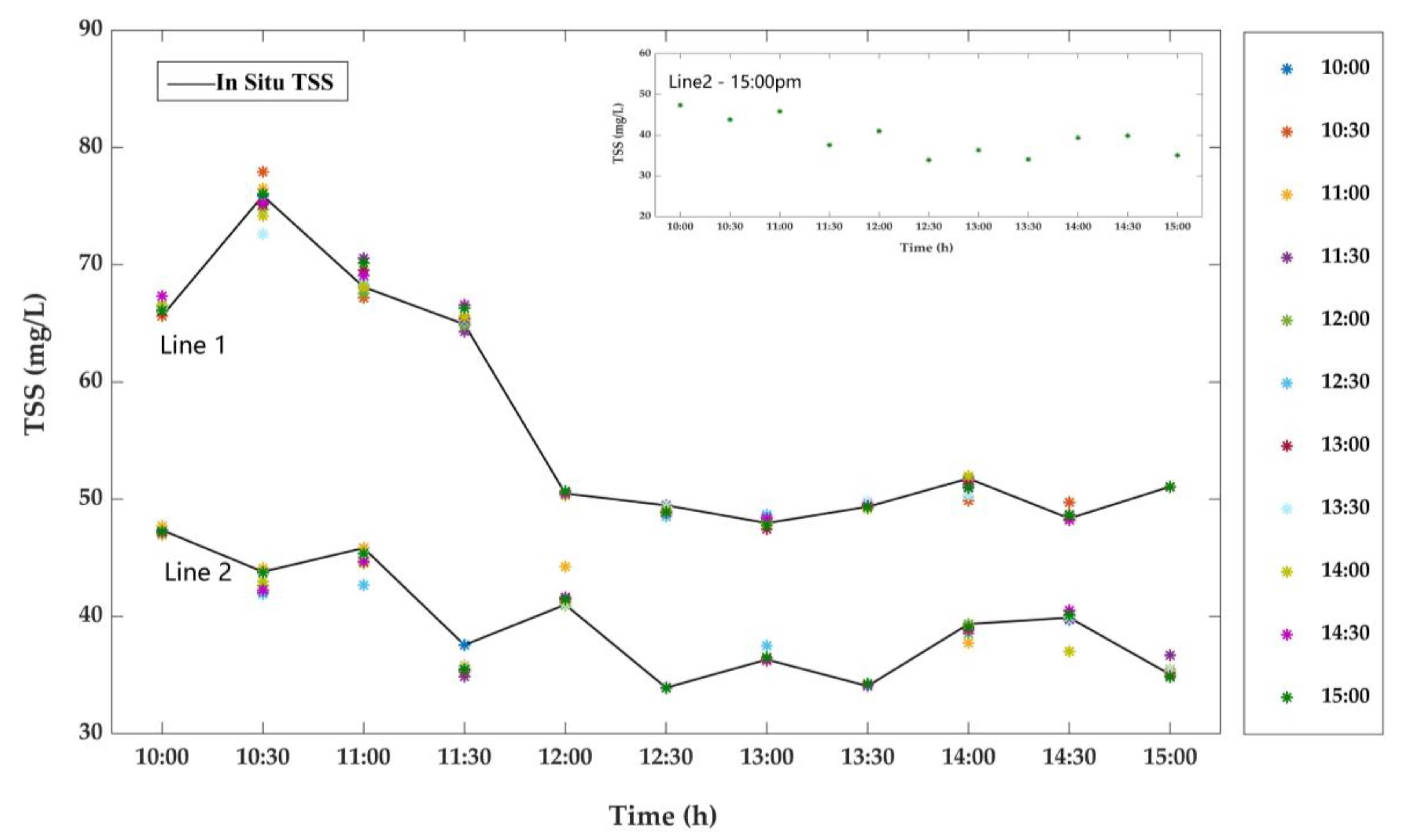
Figure 5 shows the prediction results of TSS using GRNN-based model constructed under sunny weather condition. In Figure 5, Line 1 and Line 2 show the predicted TSS at different value ranges, where TSS of Line 1 changes from 65 to 50 mg/L, Line 2 changes from 47 to 35 mg/L. The picture in the upper right corner of Figure 5 is one set of prediction results in Line 2, which is predicted based on the TSS measured at 15:00. It can be seen from Figure 5 that the GRNN-based multi-parameters forecasting model in this paper still predicts and tracks the changes of TSS well. Although some of the predicted values deviated relatively largely from the actual values, such as the predicted TSS of 10:30 and 11:00 in Line 1, this is acceptable, because the value of TSS itself is much larger and their AEs are less than 10%, which are within our tolerance range. In addition, Figure 5 shows that the daily changes of TSS are relatively large. Before validation, it is more necessary to predict the change of the in situ TSS, select the in situ TSS that meets the requirements, and find a suitable time window for the matching of satellite–ground data.

5. Discussion

5.1. Environmental Variables Affecting Chl-a and TSS

Through correlation analysis, the EVs that are closely correlated with Chl-a and TSS are used as variables to build a multi-parameter forecasting model. In fact, the effects of EVs on Chl-a and TSS are quite complex. The relationship between EVs and Chl-a/TSS are analyzed in this section, so as to better serve our model construction and lay a foundation for the subsequent research work.

5.1.1. Chl-a and Environmental Variables

According to the analysis in the all-valid dataset, WT, AWS, AT, and AP are correlated with Chl-a. Among them, WT and AT are determined by the light intensity on the water surface and are closely correlated with Chl-a. The increase of WT and AT can affect Chl-a by accelerating the rate of enzyme reaction, enhancing metabolism, and other processes of photosynthesis, so there will be a positive correlation between temperature and Chl-a [50]. According to correlation result, AWS shows a positive relationship with Chl-a. Actually, wind speed has a complicated influence on the changes of Chl-a [51]. On the one hand, wind and waves can cause resuspension of sediments in lakes. Shallow lakes like Taihu Lake are more susceptible to wind-induced waves and currents and easy to occur resuspension [52]. Resuspension will bring sedimentary particles rich in nutrients (nitrogen and phosphorus) into the water, causing the release of nutrients [53], thereby promoting the growth of phytoplankton, and corresponding Chl-a will increase. On the other hand, the change of wind speed will cause the drift of phytoplankton such as cyanobacteria, and the drift speed of cyanobacteria is increasing when AWS increases [54]. The change of AP may affect the exchange of CO 2 at the water–air surface, thereby influencing the growth of phytoplankton, and the correlation analysis result shows that AP is negatively correlated with Chl-a. In fact, the daily change of AP is quite weak when the weather condition is stable. In this paper, AP is introduced as one of modeling variables to reflect the impact of AP on changes of Chl-a on long time scales, such as seasonal changes.

5.1.2. TSS and Environmental Variables

According to the analysis in the all-valid dataset, Cond, AWS, AWD, and AT are correlated with TSS. Among them, the correlation between TSS and AWS is the most significant. For shallow lakes, wind and waves will not only accelerate the moving and mixing of lake water, but also lead to the resuspension of lake sediments, both of which will increase TSS. Therefore, there is a significant positive correlation between TSS and AWS [52]. Wind direction is related to the accumulation of phytoplankton and suspended particles, and mainly determines the spatial distribution of TSS in the lake. In different season, affected by different wind directions, the distribution of TSS is different in Taihu Lake [55]. According to the correlation analysis results, AWD and TSS show a positive correlation, but ρ is only 0.25, which is weaker than AWS. More data and researches are needed for analyzing the specific impact of AWD on TSS. In addition, Cond is a physical quantity used to characterize the conductivity of water, which will increase when there are more soluble particles such as inorganic acids, alkalis, salts, or organic conductors in water [56]. Early researches showed that conductivity is positively correlated with ion such as sulphate and nutrient such as nitrate [57]. The correlation analysis in this paper showed that Cond is negatively correlated with TSS. We believe this can be attributed to the subtle relationship between the contents of soluble and insoluble particles. Actually, the relationship between AT and TSS is indirect, changes in temperature first cause changes of phytoplankton growth. The primary production of phytoplankton generates organic particulate matter, and the suspension of organic particulate matter will increase the content of suspended solids in water [52]. TSS in this paper refers to the total suspended solids concentration in waterbodies; an increase in any one of the phytoplankton or particulate organic matter leads to an increase in TSS.

5.2. Application of Multi-Parameter Forecasting Model in Validaiton

Using long-term observation data from the site in Taihu Lake, this paper provides a model to predict the changes of Chl-a and TSS. Based on the long-term observation data of any lake site, a prediction model similar to this paper can be established. In the prediction models of Chl-a and TSS, the modeling variables are mainly composed of Chl-a t 0 , TSS t 0 , the key related EVs, and the time interval Δ t , and the selection of key EVs is most important when building the model. Although EVs such as FDOM and PC are also moderately correlated with Chl-a/TSS, they should not be considered when selecting modeling variables due to their high spatial heterogeneity in lakes [58,59]. Using the established model, we can predict the changes of the measured data in validation experiments, thereby completing the data screening and satellite–ground data matching.

5.2.1. Predicting the Changes of Chl-a and TSS

In this paper, EVs such as WT, Cond, AWS, AT, etc., used in the prediction model are all collected by buoy with a relatively fixed position. However, in actual validation experiments, the in situ data are measured by the experimental ship sailing among different sampling points, which means that the time for measuring EVs at each sampling point is different. How to use a multi-parameter forecasting model to predict the changes of in situ data in actual validation experiments is an important question.
In the validation for high- and medium-resolution satellite RSPs, the experimental areas are generally open and calm lakes and reservoirs, and the distance between sampling points is about 200–1000 m. For waterbodies, especially in open lakes, the changes of most EVs in the spatial dimension are much weaker than in the time dimension [60,61]. In this case, it is unlikely to form a small climatic field, and there will be little difference in the flow and diffusion of waterbodies between sampling points. Therefore, we can say the waterbody physical parameters such as WT, Sal, Cond, and SpC and the atmospheric environmental parameters like AT, AH, AWD, AWS, and AP measured at different sampling points are similar, and there will be very little spatial heterogeneity. Based on the above analysis, we can make the following assumptions: (1) these EVs measured at arbitrary sampling points in the experimental area can effectively represent the EVs of the whole area; (2) due to the different measuring times, these EVs measured at different sampling points can form continuous EVs of the whole experimental area. Based on these assumptions, the EVs like WT, Cond, AWS, AT, and AP, measured at different sampling points at time t, can represent the EVs of the whole experimental area and be used as input variables to predict the changes of in situ Chl-a and TSS data of a certain sampling point within the experimental area. In this kind of validation experiments, while observing water quality parameters, a portable weather station should be equipped to obtain atmospheric EVs to complete predictions.
In the validation for low-resolution satellites such as MODIS and MERIS, due to the large satellite footprint, the spacing between sampling points generally exceeds 2 km, and most of the measurements are carried out in sea and ocean. The excessive distance of sampling points and complex water environment will lead to a large difference in EVs among different points. Therefore, EVs observed at different points cannot represent the EVs of the whole experimental area. We suggest measuring EVs at all sampling points during the observed time period, so as to predict the changes of Chl-a and TSS in situ data over time on large spatial scales.

5.2.2. An Example for Screening In Situ Data

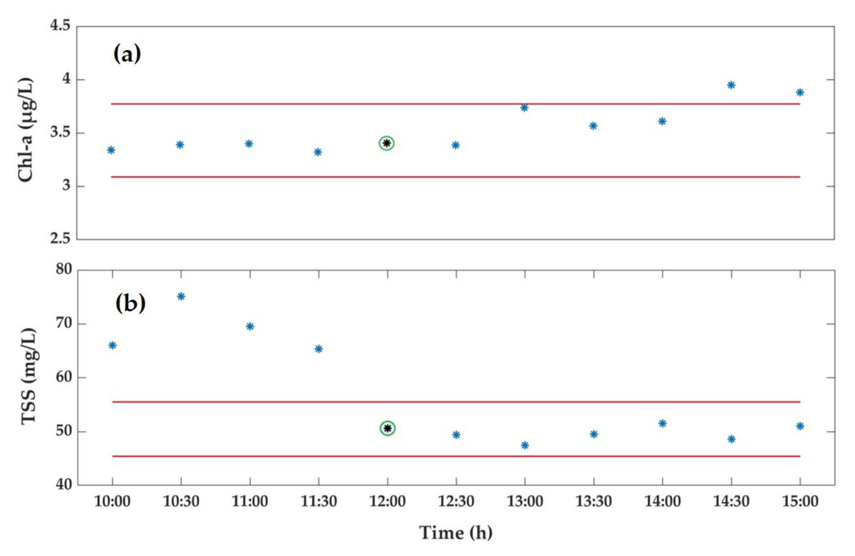
Many satellites are set to transit around 12:00 of local time, so we took the changes of in situ data measured at 12:00 as examples. In order to ensure the validating accuracy of RSPs, we assumed that the relative variations of in situ Chl-a and TSS should not exceed 10%. Figure 6 is a result of using a multi-parameter forecasting model in the sunny-day dataset to screen in situ data. In situ Chl-a and TSS measured at 12:00 are 3.42 and 50.49 mg/L, respectively. Taking them as baselines and draw boundaries with a relative change of ±10%, which are indicated by four red lines in Figure 6.
The blue dots in Figure 6a are the prediction results, which show the in situ Chl-a changes under the influence of different EVs. The corresponding EVs of that day were checked, and we found that the variations of AT and AP contributed to the increasing of Chl-a. From 10:00 to 15:00, AT was slightly increasing from 10.3 to 12.8 °C, and AP was slightly decreasing from 1018 to 1012 hpa. According to Figure 6a, the predicted values of Chl-a between 10:00 and 14:00 are within the boundary, while the Chl-a predicted at 14:30 and 15:00 exceed the boundary. Therefore, for this sampling point, the in situ Chl-a measured at 12:00 can meet the validation requirements of satellites transiting from 10:00 to 14:00, but cannot be used to verify the satellites transiting from 14:30 to 15:00.
Similarly, TSS also changes under the influence of EVs, and the changes in TSS are more dramatic. We checked the modeling EVs and found that both AWS and Cond had great changes in the morning on that day and kept small fluctuations in the afternoon. Among them, in the morning, AWS decreased from the highest 9.5 to 6 m/s and then maintained between 5 and 6 m/s in the afternoon, Cond increased from 380 to 440 μS/cm, and then maintained 430–440 μS/cm, which both explain the changes in TSS. In Figure 6b, it can be seen that the time window is 12:00–15:00 when the relative change of in situ TSS is less than 10%, which means that the in situ TSS measured at 12:00 at this sampling point can be used to verify the satellite transiting from 12:00 to 15:00, but cannot be used to validate satellites transiting before 12:00.
Correspondingly, the changes of the in situ data measured at each sampling point can be predicted. We can screen the in situ data that satisfy the relative changing criterion based on the prediction results and use it to verify the satellite that transit at a certain time. It is also possible to identify the applicable time ranges of in situ data, and to optimize the temporal window for satellite–ground data matching. The quality of in situ data can be controlled by filtering the data according to the relative changing requirements, so that the accuracy of satellite data and products can be verified more reasonably.

6. Conclusions

The reliability of in situ data is very important for the validation of remote sensing products. Under the complex environmental conditions, the constant changes of waterbody parameters over time challenge the traditional satellite–ground data matching method. In this paper, the long-term in situ data from the fixed observing site in Taihu Lake is used to analyze the environmental factors that affect the changes of Chl-a and TSS. Using the key influencing factors of each parameter obtained from the analysis, a model was constructed to predict the changes of Chl-a and TSS. At the same time, the accuracy of the model was evaluated by using the in situ data. The results show that the model based on GRNN simulation method has the highest accuracy. The prediction results of this model can intuitively show the changes of Chl-a and TSS between 10:00 and 15:00. The model in this paper is intended to provide a method for the screening of in situ data in validation of waterbody RSPs, which should not be regarded as a universal model for using EVs to fit the in situ data. By predicting the changes of Chl-a and TSS, the model can be well used for screening in situ data and providing a reference for the matching of satellite–ground data.
By establishing the prediction model, we have initially solved the reliability problem of the satellite–ground synchronization data in the validation of waterbody RSPs. However, there are some issues that require further research. First of all, due to factors such as the cost of the experimental instruments and the buoy system, we only collected in situ data from one site, so that the range of Chl-a and TSS may be not enough to represent the entire Taihu Lake. The model may lack representativeness in a large spatial range, and it may be insufficient to apply for the validation of low-resolution satellites. On the other hand, limited by the amount of data, some variables do not completely satisfy the normal distribution, and the influence of some environmental factors on the changes of Chl-a and TSS may not be sufficiently analyzed. In the future, we hope to set up more observing sites, accumulate the in situ data for a longer period of time, and analyze the relationship between EVs and Chl-a/TSS more deeply, so as to improve our model and increase the accuracy of prediction.

Author Contributions

X.Z., Z.T., and F.X. designed the research, carried out the experiments, as well as prepared the manuscript. All authors contributed to the scientific content, the interpretation of the results, and manuscript revisions. All authors have read and agreed to the published version of the manuscript.

Funding

This paper was funded by the Joint Validation of Multi-Source Remote Sensing Information and Sharing in BRICS Countries under contract No. 2018YFE0124200 and the Key Technologies for Collaborative Processing and Joint Verification of Basic Common Products of Quantitative Remote Sensing for the “Belt and Road” under contract No. 2020YFE0200700.

Institutional Review Board Statement

Not applicable.

Informed Consent Statement

Not applicable.

Data Availability Statement

The data presented in this study are available on request from the corresponding author. The data are not publicly available due to the limitation of data sharing in the fund projects.

Acknowledgments

We would like to thank the Land Observation Satellite Supporting Platform of National Civil Space Infrastructure Project for providing research data.

Conflicts of Interest

The authors declare no conflict of interest.

References

  1. Usali, N.; Ismail, M.H. Use of remote sensing and GIS in monitoring water quality. J. Sustain. Dev. 2010, 3, 228. [Google Scholar] [CrossRef]
  2. Dube, T.; Mutanga, O.; Seutloali, K.; Adelabu, S.; Shoko, C. Water quality monitoring in sub-Saharan African lakes: A review of remote sensing applications. Afr. J. Aquat. Sci. 2015, 40, 1–7. [Google Scholar] [CrossRef]
  3. Peppa, M.; Vasilakos, C.; Kavroudakis, D. Eutrophication Monitoring for Lake Pamvotis, Greece, Using Sentinel-2 Data. ISPRS Int. J. Geo Inf. 2020, 9, 143. [Google Scholar] [CrossRef] [Green Version]
  4. Zhang, Y.; Hou, Y.; Yang, X. Sea Level Rise and Coastal Infrastructure || Coastal Disasters and Remote Sensing Monitoring Methods; IntechOpen: London, UK, 2018; Chapter 8. [Google Scholar] [CrossRef]
  5. Zhang, Y.; Shi, K.; Zhang, Y.; Moreno-Madrinan, M.J.; Li, Y.; Li, N. A semi-analytical model for estimating total suspended matter in highly turbid waters. Opt. Express 2018, 26, 34094–34112. [Google Scholar] [CrossRef] [PubMed]
  6. Tao, Z.; Wang, Y.; Ma, S.; Lv, T.; Zhou, X. A Phytoplankton Class-Specific Marine Primary Productivity Model Using MODIS Data. IEEE J. Sel. Top. Appl. Earth Obs. Remote Sens. 2017, 10, 5519–5528. [Google Scholar] [CrossRef]
  7. Zheng, G.; DiGiacomo, P.M. Uncertainties and applications of satellite-derived coastal water quality products. Prog. Oceanogr. 2017, 159, 45–72. [Google Scholar] [CrossRef]
  8. Justice, C.; Belward, A.; Morisette, J.; Lewis, P.; Privette, J.; Baret, F. Developments in the ‘validation’ of satellite sensor products for the study of the land surface. Int. J. Remote Sens. 2000, 21, 3383–3390. [Google Scholar] [CrossRef]
  9. Zhang, R.; Tian, J.; Li, Z.; Su, H.; Chen, S.; Tang, X. Principles and methods for the validation of quantitative remote sensing products. Sci. China Earth Sci. 2010, 53, 741–751. [Google Scholar] [CrossRef]
  10. Privette, J.L.; Morisette, J.T.; Justice, C.; Starr, D. EOS global land validation network. In Proceedings of the IEEE 1999 International Geoscience and Remote Sensing Symposium. IGARSS’99 (Cat. No. 99CH36293), Hamburg, Germany, 28 June–2 July 1999; pp. 2587–2589. [Google Scholar]
  11. Baret, F.; Weiss, M.; Allard, D.; Garrigues, S.; Leroy, M.; Jeanjean, H.; Fernandes, R.; Myneni, R.; Privette, J.; Morisette, J. VALERI: A network of sites and a methodology for the validation of medium spatial resolution land satellite products. Remote Sens. Environ. 2005, 76, 36–39. [Google Scholar]
  12. Guillevic, P.C.; Nickeson, J.; Roman, M.; Wang, Z.; Schaepman-Strub, G. Global Land Product Validation Protocols: An Initiative of the CEOS Working Group on Calibration and Validation to Evaluate Satellite-derived Essential Climate Variables. AGUFM 2016, 2016, B33J-01. [Google Scholar]
  13. Morisette, J.T.; Privette, J.L.; Justice, C.O. A framework for the validation of MODIS land products. Remote Sens. Environ. 2002, 83, 77–96. [Google Scholar] [CrossRef]
  14. Barr, A.; Black, A.; McCaughey, H.; Amiro, B.; Hogg, T.; Murayama, S.; Iwashita, H.; Kljun, N.; Morgenstern, K.; Griffis, T. The Boreal Ecosystem Research and Monitoring Sites: A Synthesis of Results, 1994–2003. AGUSM 2004, 2004, B22A-01. [Google Scholar]
  15. Avissar, R.; Silva Dias, P.L.; Silva Dias, M.A.; Nobre, C. The large-scale biosphere-atmosphere experiment in Amazonia (LBA): Insights and future research needs. J. Geophys. Res. Atmos. 2002, 107, LBA 54-51–LBA 54-56. [Google Scholar] [CrossRef] [Green Version]
  16. Li, X.; Ma, M.; Wang, J.; Liu, Q.; Che, T.; Hu, Z.; Xiao, Q.; Liu, Q.; Su, P.; Chu, R. Simultaneous remote sensing and ground-based experiment in the Heihe River Basin: Scientific objectives and experiment design. Adv. Earth Sci. 2008, 23, 897–914. [Google Scholar]
  17. Li, X.; Liu, S.; Ma, M.; Xiao, Q.; Liu, Q.; Jin, R.; Che, T.; Wang, W.; Qi, Y.; Li, H. HiWATER: An integrated remote sensing experiment on hydrological and ecological processes in the Heihe River Basin. Adv. Earth Sci. 2012, 27, 481–498. [Google Scholar]
  18. Hu, S.; Cao, W.; Wang, G.; Xu, Z.; Lin, J.; Zhao, W.; Yang, Y.; Zhou, W.; Sun, Z.; Yao, L. Comparison of MERIS, MODIS, SeaWiFS-derived particulate organic carbon, and in situ measurements in the South China Sea. Int. J. Remote Sens. 2016, 37, 1585–1600. [Google Scholar] [CrossRef]
  19. Li, X.; Liu, Q.; Yang, R.; Wen, J.; Zhang, J.; Cai, E.; Zhang, H. The combination of ground-sensing network and satellite remote sensing in Huailai county. IEEE Sens. J. 2016, 16, 3819–3826. [Google Scholar] [CrossRef]
  20. Dou, B.; Wen, J.; Li, X.; Liu, Q.; Peng, J.; Xiao, Q.; Zhang, Z.; Tang, Y.; Wu, X.; Lin, X. Wireless sensor network of typical land surface parameters and its preliminary applications for coarse-resolution remote sensing pixel. Int. J. Distrib. Sens. Netw. 2016, 12, 9639021. [Google Scholar] [CrossRef] [Green Version]
  21. Rodeghiero, M.; Cescatti, A. Spatial variability and optimal sampling strategy of soil respiration. For. Ecol. Manag. 2008, 255, 106–112. [Google Scholar] [CrossRef]
  22. Pujar, P.M.; Kenchannavar, H.H.; Kulkarni, U.P. Wireless Sensor Network based Water Monitoring Systems: A survey. In Proceedings of the 2016 2nd International Conference on Applied and Theoretical Computing and Communication Technology (iCATccT), Bangalore, India, 21–23 July 2016. [Google Scholar]
  23. Kallio, K.; Koponen, S.; Ylöstalo, P.; Kervinen, M.; Pyhälahti, T.; Attila, J. Validation of MERIS spectral inversion processors using reflectance, IOP and water quality measurements in boreal lakes. Remote Sens. Environ. 2015, 157, 147–157. [Google Scholar] [CrossRef]
  24. Sharma, S.; Gray, D.K.; Read, J.S.; O’reilly, C.M.; Schneider, P.; Qudrat, A.; Gries, C.; Stefanoff, S.; Hampton, S.E.; Hook, S. A global database of lake surface temperatures collected by in situ and satellite methods from 1985–2009. Sci. Data 2015, 2, 1–19. [Google Scholar] [CrossRef] [PubMed] [Green Version]
  25. Bailey, S.W.; Werdell, P.J. A multi-sensor approach for the on-orbit validation of ocean color satellite data products. Remote Sens. Environ. 2006, 102, 12–23. [Google Scholar] [CrossRef]
  26. Lei, S.; Xu, J.; Li, Y.; Lyu, H.; Liu, G.; Zheng, Z.; Xu, Y.; Du, C.; Zeng, S.; Wang, H. Temporal and spatial distribution of Kd (490) and its response to precipitation and wind in lake Hongze based on MODIS data. Ecol. Indic. 2020, 108, 105684. [Google Scholar] [CrossRef]
  27. Sun, L.; Wang, X.; Guo, M.; Tang, J. MODIS ocean color product validation around the Yellow Sea and East China Sea. J. Lake Sci. 2009, 21, 298–306. [Google Scholar]
  28. Zhao, W.; Wang, G.; Cao, W.; Cui, T.; Wang, G.; Ling, J.; Sun, L.; Zhou, W.; Sun, Z.; Xu, Z. Assessment of SeaWiFS, MODIS, and MERIS ocean colour products in the South China Sea. Int. J. Remote Sens. 2014, 35, 4252–4274. [Google Scholar] [CrossRef]
  29. Palmer, S.C.; Hunter, P.D.; Lankester, T.; Hubbard, S.; Spyrakos, E.; Tyler, A.N.; Presing, M.; Horváth, H.; Lamb, A.; Balzter, H. Validation of Envisat MERIS algorithms for chlorophyll retrieval in a large, turbid and optically-complex shallow lake. Remote Sens. Environ. 2015, 157, 158–169. [Google Scholar] [CrossRef] [Green Version]
  30. Yu, G.; Yang, W.; Matsushita, B.; Li, R.; Oyama, Y.; Fukushima, T. Remote estimation of Chlorophyll-a in inland waters by a NIR-Red-based algorithm: Validation in Asian lakes. Remote Sens. 2014, 6, 3492–3510. [Google Scholar] [CrossRef] [Green Version]
  31. Zheng, Z.; Ren, J.; Li, Y.; Huang, C.; Liu, G.; Du, C.; Lyu, H. Remote sensing of diffuse attenuation coefficient patterns from Landsat 8 OLI imagery of turbid inland waters: A case study of Dongting Lake. Sci. Total Environ. 2016, 573, 39–54. [Google Scholar] [CrossRef]
  32. Cheng, C.; Wei, Y.; Lv, G.; Xu, N. Remote sensing estimation of chlorophyll-a concentration in Taihu Lake considering spatial and temporal variations. Environ. Monit. Assess. 2019, 191, 84. [Google Scholar] [CrossRef]
  33. Xia, R.; Li, Y.-M.; Wu, C.-Q.; Jin, X.; Wang, Y.-f. Spatial Distribution and Variation of Concentration of Suspended Solids in Taihu Lake based on HJ-1 Satellite Data. Sci. Geogr. Sin. 2011, 31, 197–203. [Google Scholar]
  34. Xu, Y.; Qin, B.; Zhu, G.; Zhang, Y.; Shi, K.; Li, Y.; Shi, Y.; Chen, L. High temporal resolution monitoring of suspended matter changes from GOCI measurements in Lake Taihu. Remote Sens. 2019, 11, 985. [Google Scholar] [CrossRef] [Green Version]
  35. Seo, S. A Review and Comparison of Methods for Detecting Outliers in Univariate Data Sets. Master’s Thesis, University of Pittsburgh, Pittsburgh, PA, USA, 2006. [Google Scholar]
  36. Senthilnathan, S. Usefulness of Correlation Analysis. SSRN Electron. J. 2019, 1–9. [Google Scholar] [CrossRef]
  37. Jones, M.P. Indicator and Stratification Methods for Missing Explanatory Variables in Multiple Linear ReGression. Pub. Am. Stat. Assoc. 1996, 91, 222–230. [Google Scholar] [CrossRef]
  38. Panda, S.; Amatya, D.M.; Jackson, R.; Sun, G.; Noormets, A. Automated geospatial models of varying complexities for pine forest evapotranspiration estimation with advanced data mining. Water 2018, 10, 1687. [Google Scholar] [CrossRef] [Green Version]
  39. Wang, W.; Zhao, S.; Jiao, L.; Taylor, M.; Zhang, B.; Xu, G.; Hou, H. Estimation of PM2. 5 concentrations in China using a spatial back propagation neural network. Sci. Rep. 2019, 9, 1–10. [Google Scholar]
  40. Yang, L.; Jia, K.; Liang, S.; Wei, X.; Yao, Y.; Zhang, X. A robust algorithm for estimating surface fractional vegetation cover from landsat data. Remote Sens. 2017, 9, 857. [Google Scholar] [CrossRef] [Green Version]
  41. Zhang, Z.; Gong, Y.; Wang, Z. Accessible remote sensing data based reference evapotranspiration estimation modelling. Agric. Water Manag. 2018, 210, 59–69. [Google Scholar] [CrossRef]
  42. Yuan, Q.; Shen, H.; Li, T.; Li, Z.; Li, S.; Jiang, Y.; Xu, H.; Tan, W.; Yang, Q.; Wang, J. Deep learning in environmental remote sensing: Achievements and challenges. Remote Sens. Environ. 2020, 241, 111716. [Google Scholar] [CrossRef]
  43. Özerdem, M.S.; Acar, E.; Ekinci, R. Soil moisture estimation over vegetated agricultural areas: Tigris Basin, Turkey from Radarsat-2 data by polarimetric decomposition models and a generalized regression neural network. Remote Sens. 2017, 9, 395. [Google Scholar] [CrossRef] [Green Version]
  44. Xiao, Z.; Liang, S.; Wang, J.; Chen, P.; Yin, X.; Zhang, L.; Song, J. Use of general regression neural networks for generating the GLASS leaf area index product from time-series MODIS surface reflectance. IEEE Trans. Geosci. Remote Sens. 2013, 52, 209–223. [Google Scholar] [CrossRef]
  45. Li, T.; Shen, H.; Zeng, C.; Yuan, Q.; Zhang, L. Point-surface fusion of station measurements and satellite observations for mapping PM2.5 distribution in China: Methods and assessment. Atmos. Environ. 2017, 152, 477–489. [Google Scholar] [CrossRef] [Green Version]
  46. Al-Mahasneh, A.J.; Anavatti, S.G.; Garratt, M.A. Review of Applications of Generalized Regression Neural Networks in Identification and Control of Dynamic Systems. arXiv 2018, arXiv:1805.11236. [Google Scholar]
  47. Chen, M.; Fan, M.; Liu, R.; Wang, X.; Yuan, X.; Zhu, H. The dynamics of temperature and light on the growth of phytoplankton. J. Theor. Biol. 2015, 385, 8–19. [Google Scholar] [CrossRef] [PubMed]
  48. Chen, J.Y.; Wang, S.H.; Jiang, X.; Huang, X.F.; Zhao, L. Fluorescence Spectral Characteristics of Fluorescent Dissolved Organic Matter (FDOM) in the Surface Sediments from Lihu Lake. Huanjing Kexue 2017, 38, 70–77. [Google Scholar]
  49. Wang, J.; Shi, R.; Gao, W. Retrieval of phycocyanin concentration in the eutrophic Taihu Lake. In Proceedings of the Remote Sensing and Modeling of Ecosystems for Sustainability XI, San Diego, CA, USA, 8 October 2014; p. 92210Z. [Google Scholar]
  50. Wu, Q.; Xia, X.; Li, X.; Mou, X. Impacts of meteorological variations on urban lake water quality: A sensitivity analysis for 12 urban lakes with different trophic states. Aquat. Sci. 2014, 76, 339–351. [Google Scholar] [CrossRef]
  51. Chiswell, S.M.; Zeldis, J.R.; Hadfield, M.G.; Pinkerton, M.H. Wind-driven upwelling and surface chlorophyll blooms in Greater Cook Strait. N. Z. J. Mar. Freshw. Res. 2017, 51, 465–489. [Google Scholar] [CrossRef]
  52. Tammeorg, O.; Niemistö, J.; Möls, T.; Laugaste, R.; Panksep, K.; Kangur, K. Wind-induced sediment resuspension as a potential factor sustaining eutrophication in large and shallow Lake Peipsi. Aquat. Sci. 2013, 75, 559–570. [Google Scholar] [CrossRef]
  53. Søndergaard, M.; Jensen, J.P.; Jeppesen, E. Role of sediment and internal loading of phosphorus in shallow lakes. Hydrobiologia 2003, 506, 135–145. [Google Scholar] [CrossRef]
  54. Yu, M.-L.; Hong, G.-X.; Zhu, G.-W.; Quan, Q.-M.; Xu, H.; Zhu, M.-Y.; Ding, W.-H.; Li, W.; Wu, T.-F. Wind Field Influences on the Spatial Distribution of Cyanobacterial Blooms and Nutrients in Meiliang Bay of Lake Taihu, China. Huanjing Kexue 2019, 40, 3519. [Google Scholar]
  55. Shi, K.; Zhang, Y.; Zhu, G.; Liu, X.; Zhou, Y.; Xu, H.; Qin, B.; Liu, G.; Li, Y. Long-term remote monitoring of total suspended matter concentration in Lake Taihu using 250 m MODIS-Aqua data. Remote Sens. Environ. 2015, 164, 43–56. [Google Scholar] [CrossRef]
  56. Company, H. Hach Water Analysis Handbook; Hach Company: Loveland, CO, USA, 1992. [Google Scholar]
  57. Shuhaimi-Othman, M.; Lim, E.C.; Mushrifah, I. Water quality changes in Chini lake, Pahang, west Malaysia. Environ. Monit. Assess. 2007, 131, 279–292. [Google Scholar] [CrossRef] [PubMed]
  58. Kim, J.; Kim, G. Inputs of humic fluorescent dissolved organic matter via submarine groundwater discharge to coastal waters off a volcanic island (Jeju, Korea). Sci. Rep. 2017, 7, 7921. [Google Scholar] [CrossRef] [PubMed] [Green Version]
  59. Randolph, K.; Wilson, J.; Tedesco, L.; Li, L.; Pascual, D.L.; Soyeux, E. Hyperspectral remote sensing of cyanobacteria in turbid productive water using optically active pigments, chlorophyll a and phycocyanin. Remote Sens. Environ. 2008, 112, 4009–4019. [Google Scholar] [CrossRef]
  60. Xu, X.; Tao, R.; Zhao, Q.; Wu, T. Wave characteristics and sensitivity analysis of the wind field in a large shallow lake- Lake Taihu. J. Lake Sci. 2013, 25, 55–64. [Google Scholar]
  61. Wang, W.; Xiao, W.; Cao, C.; Gao, Z.; Hu, Z.; Liu, S.; Shen, S.; Wang, L.; Xiao, Q.; Xu, J. Temporal and spatial variations in radiation and energy balance across a large freshwater lake in China. J. Hydrol. 2014, 511, 811–824. [Google Scholar] [CrossRef]
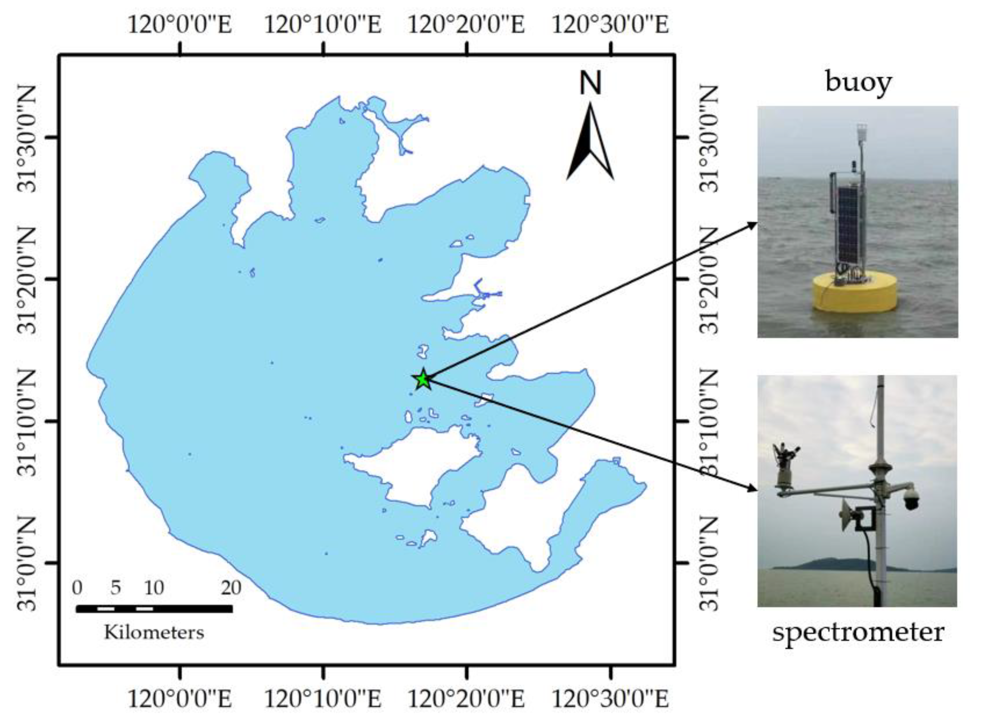
Figure 1. Location of the experimental area and the measuring instruments in Taihu Lake.
Remotesensing 13 00070 g001
Figure 2. Accuracy evaluation of multi-parameters forecasting models for sunny-day Chl-a based on (a) MLR, (b) BPNN, and (c) GRNN.
Remotesensing 13 00070 g002
Figure 3. Accuracy evaluation of multi-parameters forecasting models for sunny-day TSS based on (a) MLR, (b) BPNN, and (c) GRNN.
Remotesensing 13 00070 g003
Figure 4. Prediction of Chl-a by GRNN-based multi-parameters forecasting model in sunny-day dataset. Lines 1, 2, and 3 show predicted Chl-a at different concentration ranges, respectively.
Remotesensing 13 00070 g004
Figure 5. Prediction of TSS by GRNN-based multi-parameters forecasting model in a sunny-day dataset. Lines 1 and 2 show predicted TSS at different concentration ranges, respectively.
Remotesensing 13 00070 g005
Figure 6. An example of in situ data screening using the multi-parameters forecasting model of (a) Chl-a and (b) TSS, where the black dots represent in situ Chl-a and TSS, and the blue dots refer to the predicted Chl-a and TSS based in situ Chl-a and TSS, respectively. In addition, the red lines represent the boundary of ±10% relative change, which are drawn based on in situ Chl-a and TSS measured at 12:00 (marked with green circles in the figure).
Remotesensing 13 00070 g006
Table 1. Correlation analysis of the available variables WT, SpC, Cond, Sal, PC, FDOM, AWD, AWS, AT, AH, and AP in all-valid dataset.
ρ of Chl-a
and others
WTSpCCondSalPCFDOM
0.49−0.390.48−0.340.08−0.25
TSSAWDAWSATAHAP
0.08−0.100.330.47−0.08−0.43
ρ of TSS
and others
WTSpCCondSalChl-aPC
−0.25−0.01−0.27−0.030.090.08
FDOMAWDAWSATAHAP
−0.290.250.37−0.250.060.14
Table 2. Correlation analysis among selected variables WT, SpC, Cond, Sal, FDOM, AWD, AWS, AT, and AP in all-valid dataset, and several key correlation coefficients are shown in bold in the table.
WTSpCCondSalFDOMAWDAWSATAP
WT1.00
SpC−0.321.00
Cond0.90−0.311.00
Sal−0.550.98−0.181.00
FDOM−0.180.08−0.160.091.00
AWD−0.120.13−0.080.10−0.061.00
AWS0.110.070.030.01−0.17−0.021.00
AT0.96−0.400.89−0.44−0.16−0.140.071.00
AP−0.330.24−0.320.320.330.11−0.11−0.251.00
Table 3. Accuracy evaluation of multi-parameters forecasting models for all-valid Chl-a.
MethodModel ExpressionAccuracy R 2 RMSEAE
MLR Chl-a tm   =   0.82     Chl-a t 0   +   0.0126     Δ t   +   0.0154
WT + 0.0002 SpC + 0.0265 AWS +
0.0023     AP     2.9163
Train (12,653)0.780.4817.2%
Test (2460)0.720.6318.9%
BPNN Chl-a tm   =   BPNN ( Chl-a t 0 , Δ t , WT , SpC , AWS , AP )   Train (12,653)0.880.3613.2%
Test (2460)0.810.5415.6%
GRNN Chl-a tm   =   GRNN ( Chl-a t 0 , Δ t , WT , SpC , AWS , AP )   Train (12,653)0.980.188.2%
Test (2460)0.850.4111.4%
Table 4. Accuracy evaluation of multi-parameters forecasting models for all-valid TSS.
MethodModel ExpressionAccuracy R 2 RMSEAE
MLR TSS tm = 0.90 TSS t 0 0.5367 Δ t 0.0106
Cond + 0.0016 AWD + 0.5157 AWS +
5.4838
Train (10,078)0.887.8217.2%
Test (1865)0.868.6717.3%
BPNN TSS tm = BPNN ( TSS t 0 , Δ t , Cond , AWD , AWS )   Train (10,078)0.936.5214.4%
Test (1865)0.896.8614.6%
GRNN TSS tm = GRNN ( TSS t 0 , Δ t , Cond , AWD ,   AWS )   Train (10,078)0.964.278.9%
Test (1865)0.906.2011.3%
Table 5. Correlation analysis of the available variables WT, SpC, Cond, Sal, PC, FDOM, AWD, AWS, AT, AH, and AP in sunny-day dataset.
ρ of Chl-a
and others
WTSpCCondSalPCFDOM
0.30−0.070.13−0.090.44−0.19
TSSAWDAWSATAHAP
0.25−0.150.370.310.16−0.33
ρ of TSS
and others
WTSpCCondSalChl-aPC
−0.26−0.08−0.21−0.040.240.51
FDOMAWDAWSATAHAP
−0.32−0.070.38−0.31−0.140.17
Table 6. Correlation analysis among selected variables WT, Cond, AWS, AT, and AP in sunny-day dataset, and several key correlation coefficients are shown in bold in the table.
WTCondAWSATAP
WT1.00
Cond0.631.00
AWS0.230.061.00
AT0.860.240.201.00
AP−0.29−0.26−0.28−0.241.00
Table 7. The testing accuracy of GRNN-based model built according to different | Δ t | in the all-valid and the sunny-day datasets
| Δ t | . | Δ t |     1   h 1   h   <   | Δ t |     2   h 2   h   <   | Δ t |     3   h 3   h   <   | Δ t |     4   h 4   h   <   | Δ t |     5   h
ParameterChl-aTSSChl-aTSSChl-aTSSChl-aTSSChl-aTSS
All-validNum.53544217414132332967238218491460802651
R20.940.950.930.940.900.920.870.860.850.85
RMSE0.234.610.294.970.315.560.345.820.406.01
AE7.4%8.2%9.3%9.1%9.9%10.4%10.3%11.5%11.9%12.3%
Sunny-dayNum.12491133965894675657417394193168
R20.970.950.960.820.930.900.890.890.880.86
RMSE0.204.280.224.690.264.870.295.750.305.96
AE5.9%6.3%7.2%7.1%8.1%7.7%8.5%8.3%9.1%8.7%
Publisher’s Note: MDPI stays neutral with regard to jurisdictional claims in published maps and institutional affiliations.