Individual Tree Diameter Estimation in Small-Scale Forest Inventory Using UAV Laser Scanning

Abstract

Unmanned aerial vehicle laser scanning (UAVLS) systems present a relatively new means of remote sensing and are increasingly applied in the field of forest ecology and management. However, one of the most essential parameters in forest inventory, tree diameter at breast height (DBH), cannot be directly extracted from aerial point cloud data due to the limitations of scanning angle and canopy obstruction. Therefore, in this study DBH-UAVLS point cloud estimation models were established using a generalized nonlinear mixed-effects (NLME) model. The experiments were conducted using Larix olgensis as the subject species, and a total of 8364 correctly delineated trees from UAVLS data within 118 plots across 11 sites were used for DBH modeling. Both tree- and plot-level metrics were obtained using light detection and ranging (LiDAR) and were used as the models’ independent predictors. The results indicated that the addition of site-level random effects significantly improved the model fitting. Compared with nonparametric modeling approaches (random forest and k-nearest neighbors) and uni- or multivariable weighted nonlinear least square regression through leave-one-site-out cross-validation, the NLME model with local calibration achieved the lowest root mean square error (RMSE) values (1.94 cm) and the most stable prediction across different sites. Using the site in a random-effects model improved the transferability of LiDAR-based DBH estimation. The best linear unbiased predictor (BLUP), used to conduct local model calibration, led to an improvement in the models’ performance as the number of field measurements increased. The research provides a baseline for unmanned aerial vehicle (UAV) small-scale forest inventories and might be a reasonable alternative for operational forestry.

1. Introduction

Forests, as one of the essential elements of a terrestrial ecosystem, have a crucial role in terms of regulating fluxes and stores of carbon and water, contributing to biodiversity conservation, and regulating the global climate system [1,2]. To quantitatively assess the amount and map the distribution of forest and its changes, a timely and accurate forest resource inventory is needed [2].

Traditionally, forest inventories depend on the sampling of the ground truth (in situ measurements), where each selected individual’s attributes are obtained through tree-by-tree measurements [3,4]. Such inventories are not cost-effective since the field measurements are often labor-intensive and time-consuming, consequently limiting the sampling intensity and number of tree attributes measured [4]. Developments in remote sensing technologies have brought about massive breakthroughs in terms of improving the performance of forest inventory, specifically with respect to the measurement scale and efficiency [5]. Airborne LiDAR is capable of reconstructing the detailed 3D structure of the entire forest landscape using airplane-mounted high-frequency laser scanners, which might potentially overtake traditional in situ forest inventory since they can collect more information at a high resolution and accuracy in a relatively brief period [6,7,8]. Furthermore, advanced sensors and computational technology are able to accurately detect and quantify the crown dimensions of a single tree depending on the crown delineation algorithms utilized [9]. The detailed single tree-level attributes can now be directly measured, which may fundamentally shift our way of censusing forests [9,10].

In the last few years, unmanned aerial vehicles (UAVs), as a small-scale, low-cost, remote sensing alternative to satellite and airborne platforms, have provided a unique combination of high temporal and spatial resolution and have gradually become one of the most powerful tools for 3D forest mapping [11,12]. The miniaturized laser scanning sensors on UAV platforms have earned a good reputation in the field of forest inventory and surveying due to their various benefits, such as increased point densities, lower cost, flight route flexibility, and simple operation [13,14]. Compared with airborne laser scanning, UAVLS systems can obtain higher-density point cloud data at a local scale with a smaller bias and standard deviation when quantifying the crown structures, and thus have been increasingly applied for monitoring and estimating forest attributes [15,16,17].

Tree diameter at breast height (DBH) is universally known as one of the most crucial elements in forest inventories. DBH is important both ecologically and economically, in that its distribution characterizes the growth, structure, and economic merit of the stand and plays a critical role in forestry practitioners’ decision-making [18,19]. However, the utilization of aerial point clouds to measure DBH is still inadequate in terms of accuracy, since tree stems are normally occluded by canopy obstruction [20]. Without DBH measurements, established models such as tree height, taper, stem volume, biomass, and carbon storage equations can no longer be used, since DBH mostly acts as the key predictor [21,22]. Thus, estimating individual tree diameter has been a key concern in the field of forestry remote sensing [23].

Recently, an increasing number of studies have applied LiDAR data to estimate DBH [24,25]. LiDAR-derived tree height is often utilized as the preferred predictor for DBH estimation due to the strong relationship between DBH and tree height and the robustness of LiDAR height measurements [23,26]. However, using tree height as the sole predictor was found to be unreliable in predicting the DBH of large trees, since trees with a similar height might vary highly in terms of diameter [21,22]. This might be caused by the tree’s natural traits: a tree rapidly gains height to escape the understory position but then resumes expanding in diameter throughout its whole life after reaching its maximum height [27]. Thus, some researchers have suggested using crown metrics as an additional predictor for LiDAR-derived DBH estimation [22,28,29]. Furthermore, Lo and Lin (2013) proposed competition indices for evaluating whether the surrounding trees (i.e., competitors) had a significant effect on the DBH growth in an old-growth stand [25]. The environment and competition of trees indeed play vital roles in the size of an individual tree’s DBH, which should be considered when developing a DBH model [24,30,31].

With respect to LiDAR-based DBH modeling approaches, linear equations or equations that are transferable into linear forms such as exponential or power functions are often applied as regression models [21]. However, these equations may be simplistic and applicable to only a limited range of tree sizes and stand conditions [21]. Furthermore, ordinary least squares (OLS) approaches are often used to estimate parameters in these equations. Modeling data are often hierarchically/longitudinally structured, and individual trees are nested within the block level. It is difficult to satisfactorily regress the error hypothesis simultaneously, which may cause significantly biased variance estimates [32,33]. In addition, many studies have focused on using nonparametric approaches for DBH estimation. Vauhkonen et al. (2010) applied k-most similar neighbors (MSN) imputation and random forest methods to predict DBH and other attributes in Finland [34]. Yu et al. (2011) predicted tree-level attributes from airborne LiDAR point clouds using random forest approaches and achieved a similar performance with a linear regression method [35]. Although nonparametric approaches involve fewer assumptions and could achieve a higher prediction accuracy, they are not a suitable tool to understand the relationship between LiDAR metrics and forest inventory attributes [36].

One of the inherent problems with using remote sensing data as predictors is the calibration and transferability of the established equations [37,38]. Models generally perform well in regions where the modeling data are located [39]. However, practical inventories are mostly performed using different sensors or imaging parameters, and the structure of the stand- and tree-level attributes can be remarkably varied between sites [38]. Different laser scanning devices, modes, and operational parameters may generate notably distinctive point clouds [40,41,42]. Point cloud-based estimations produced by a particular device or parameter might have a higher accuracy in some sites than in others [39]. Thus, the utilization of established equations often leads to bias and is less accurate; on some occasions, the decrease is trivial and still acceptable [39]. Furthermore, forest structure can also be a source of transferability problems, mainly if there is a considerable difference between the source and the target locations, or if the model fitting data do not properly cover the variations in the data used for model validation [38,39].

In UAVLS-based forest inventories, more attention should be paid to the transferability of the model, since UAVLS acquisition is primarily affected by several environmental factors. Moreover, UAVLS is more suitable for inventorying small forest areas with a high accuracy, and it is practical to use the existing models and the new UAVLS acquisition for predicting certain variables. Our study thus focuses on developing a DBH estimation model for UAVLS-based forest inventories. The aims of the present research were to (1) delineate individual trees and extract various tree- and plot-level metrics derived from UAVLS data, (2) present a nonlinear mixed-effects (NLME) modeling framework for estimating individual tree DBH using UAVLS-derived metrics and random effects, (3) calibrate and assess the established NLME model using the field data from a different region, and (4) compare the accuracies and transferability of the DBH estimation with alternative modeling approaches. This study could provide a baseline and new perspective for DBH modeling using UAVLS for small forest inventories.

2. Materials and Methods

2.1. Study Area and UAVLS Data Acquisition

This research was conducted in Mengjiagang Forest Farm (130°32′0″–130°52′6″ E, 46°20′20″–45°30′16″ N), which is located along the western fringes of Wanda mountain in the northeastern part of Huanan County, Heilongjiang province, China. The terrain mainly features gentle slopes and low-elevation hills, with an average elevation of approximately 250 m a.s.l. [43]. The forest vegetation in the area is dominated by coniferous plantations, predominantly Pinus sylvestris var. mongolica, Pinus koraiensis, Larix olgensis, and Picea asperata.

In the present study, we used larch, one of the most abundant and economically important species in northeast China, for DBH modeling. A total of 11 sites of larch plantations of different age groups, stand densities, and forest conditions were selected to represent all larch stands in the study area (Figure 1). All the sites were dominantly covered by Larix olgensis plantations with an initial planting spacing of 2 × 1.5 m (3300 stems/ha). The stand densities were adjusted by thinning practice depending on the growth stage and site quality, which were about 3000, 2000, 1000, 700, and 500 stems/ha for young, middle-aged, near-mature, mature, and over-mature forests, respectively.

UAVLS data were acquired for these 11 sites from 10 to 12 July 2019, using a RIEGL mini VUX-1UAV LiDAR scanner (www.riegl.com/products/unmanned-scanning/riegl-minivux-1uav) carried by a Feima D200 UAV platform. The LiDAR sensor operated at a 100 kHz pulse repetition rate with a maximum scan speed of 100 scans per second. The scanner’s maximum measurement range was 250 m with an accuracy of 15 mm. All the flights were designed as crossed transects with 80 m swath overlaps at 80 m altitude and 5.0 m/s speed, conditions which are commonly used in UAVLS data collection [13,15]. The sensor provides a 360° field of view. In interpreting the point cloud data, the scanning angle was specifically set to different sites depending on the trajectory and overlaps, but all were within ±60° to avoid measurement errors caused by excessive angle. The average pulse densities for each site ranged from about 120 to 220 pulses/m², and the final point densities were about 150 to 270 pt/m², with up to five echoes. The descriptions of forest characteristics and UAVLS point densities are listed in

Table 1. Description of the forest characteristics and unmanned aerial vehicle laser scanning (UAVLS) data for a total of 11 sites.

Site	Number of Plots	Area (ha)	Structure	DBH Range (cm)	DBH Mean (cm)	CD Range (m)	CD Mean (m)	H Range (m)	H Mean (m)	Point Density (pt/m2)
1	8	9.8	Mid	5.0–23.5	11.4	1.1–6.2	2.6	5.0–19.7	12.9	155.2
2	10	9.4	Ma	18.4–40.2	27.1	1.5–8.7	4.1	18.5–30.5	25.4	187.3
3	6	6.4	Mid, Y	5.1–29.6	11.8	0.7–6.6	2.7	7.0–21.3	13.4	165.8
4	9	9.5	NM	10.5–35.2	20.8	1.2–8.5	3.4	12.0–26.3	20.3	202.1
5	14	16.3	Ma, Y	5.0–37.8	12.4	0.6–7.8	3.3	6.0–32.5	20.4	214.6
6	10	9.7	OM, Y	5.0–37.4	18.0	0.7–8.6	3.4	5.2–33.3	22.3	267.0
7	9	10.0	Ma, Mid	7.8–34.8	20.4	1.2–7.2	3.3	5.5–28.9	21.1	221.3
8	6	8.9	Ma	8.1–39.4	18.8	1.3–8.3	3.6	10.2–26.6	21.5	165.7
9	13	11.9	Nm	10.2–35.1	18.4	1.1–6.0	2.8	11.3–28.0	22.2	200.6
10	14	9.6	Y, Mid	5.0–26.1	10.6	0.7–5.0	2.4	5.1–23.6	11.5	189.9
11	19	22.4	Mid, Y	5.1–25.0	12.0	0.8–5.2	2.4	5.5–21.7	14.9	222.0
Total	118	123.7	Y, Mid, NM, Ma, OM	5.0–39.4	14.9	0.6–8.7	2.7	5.0–33.3	14.7	203.6

Note: DBH: tree diameter at breast height; CD: crown diameter; H: total tree height; Y, Mid, NM, Ma, and OM present young, middle-aged, near-mature, mature, and over-mature forests, respectively.

for each site.

2.2. In Situ Measurements

A total of 118 plots (30 m × 30 m) across 11 experimental sites were established in July 2019. The sample plots were evenly distributed in each site, excluding the edge of the stand and large forest gaps. The distance between plots was larger than twice each site’s average tree height. The number of plots for each site is listed in Table 1. DBH and crown width measurements were conducted for all trees with DBH more than 5 cm using a diameter tape. Meanwhile, the height of the first live branch position (at crown base) and the total tree height were measured using a Vertex IV instrument with a height resolution of 0.1 m (Haglöfs, Sweden). The trees’ coordinates were recorded by measuring their relative position to the corner of plots. Furthermore, the geographical coordinates of the individual trees and four corners of each plot were determined with a real-time kinetic (RTK) global navigation satellite system (GNSS) (UniStrong G10A, Beijing, China) with a positioning error of approximately 0.1 m. Trees under poor GNSS signals were georeferenced by their relative coordinates, the positioning accuracy of which was estimated to be about 0.3‒0.5 m.

2.3. LiDAR Metrics Extraction

In this study, both tree- and plot-level metrics were extracted from the UAVLS data. The tree-level metrics include the basic characteristics of each individual and their competitive status within the sample plot. In addition, stand conditions also affect individual stem diameter growth and size distribution. The plot-level metrics were used to describe the crown structural and topography characteristics that were introduced as auxiliary information.

2.3.1. UAVLS Data Preprocessing

Firstly, the noise points were manually removed from the raw LiDAR point clouds. The cloth simulation filtering was utilized to categorize the remaining points into nonground and ground points [44]. Due to the dense canopy cover, the ground point cloud density is about 10 pt/m² on average. Then, the Kriging method with a 0.5 m pixel size was used to interpolate the ground points into digital terrain models (DTMs) [45]. DTM values were subtracted to obtain the normalized height of each point [46,47]. As mentioned in early studies, data pits in the canopy height models (CHMs) disrupt the crowns’ integrity and smoothness (Figure a), which negatively affects the individual crown delineation and parameter extraction [47,48]. We therefore applied graph-based progressive morphological filtering (GPMF), a canopy filtering technique, to generate CHMs from the UAVLS data [47]. This algorithm employs an adaptive morphological operation to eliminate depression points from all returns in progressive filtering. All the remaining surface points were then interpolated by triangulated irregular networks. Many studies have generated CHM from UAVLS data with various spatial resolutions, ranging 0.1 to 1 m [10,16,49,50]. Yin and Wang (2019) have recommended that spatial resolution should be finer than one fourth of the crown diameter to correctly delineate crown boundaries and characterize the crown shapes. The grid cell should also not be much smaller than the average pulse spacing [51]. In our study, the CHMs were therefore generated at a resolution of 0.1 m, which could recognize the minimum crown diameter of 0.6 m recorded in the field survey (Table 1) and was sufficiently supported by the lowest pulse spacing of 0.09 m. As shown in Figure 2b, canopy surfaces could be characterized clearly and with few data pits.

2.3.2. Individual Tree Delineation

In recent years, two main categories of individual tree delineation methods (point cloud- and CHM-based) have been developed for ALS data [9]. Although point cloud-based algorithms are capable of capturing the understory trees under main canopies, a huge amount of computation and complex parameters limit the application’s efficiency, especially for high-density UAVLS point clouds. CHM-based individual tree delineation methods were applied in this study since, in a larch plantation, there are only a few understory trees. Zhao et al. (2017) constructed a single-tree automatic detection algorithm called region-based hierarchical cross-section analysis [52]. This particular algorithm used horizontal relationships between the crown within the vertical direction, and the CHM was considered as a mountain-like topographic surface for detecting an individual tree. In order to avoid the influence of shrubs in the segmentation process, the height of the crown for automatic segmentation was limited to 3 m.

2.3.3. Tree-to-Tree Matching

All the sample trees that met the modeling’s requirements were screened using a tree-to-tree matching procedure, harmonizing the field-measured data and the segmented trees based on spatial locations and height differences [53]. The segmented trees were assigned as candidates of a reference tree if the horizontal distance from the reference was less than the corresponding crown radius (with an upper limit of 3 m); meanwhile, the height difference from the reference was less than 20% of the top height of the plot [54]. A unique candidate or the closest one among multiple candidates was selected as a match with the reference tree [47]. Segmented trees without a link to references were considered commission errors (Figure 3). Conversely, reference trees that were not matched to any segmented trees were classified as omission errors (Figure 3). In total, 8785 trees were correctly matched with the field measurements; 56–100% (mean 76%) of the trees were detected among a total of 118 plots with commission errors of 17–45% (mean 28%). As shown in Figure 3, the relatively high commission errors in our study were mainly due to the trees outside the plot, but their crowns extending into plot boundaries were mistaken as individual trees. After the matching was completed, all irrelevant trees, such as dead trees, miscellaneous trees, and incomplete segmented crowns along plot boundaries, were manually removed from the matching tree datasets. Overall, 8364 trees were selected for further modeling.

2.3.4. Tree- and Plot-Level Metrics Generation

In this study, a total of 100 UAVLS-based tree- and plot-level variables were calculated as potential predictors for future modeling. The laser returns falling within each segment were masked to clip out an individual tree and utilized to determine a set of tree-level metrics. The total height ($H$) of each individual tree was defined as the maximum height of all LiDAR pulses. The relative root mean square error between the LiDAR-derived and field-measured height was about 7% (Supplementary Materials Figure S1). A 2D convex hull of projected individuals’ points on the x‒y plane was constructed as a crown polygon [55]. Crown diameter ($CD$) was calculated by $2\times \sqrt{crown area/\pi }$, where $crown area$ was the area of the individual convex hull [56]. Moreover, the crown volume and surface area [26,47] and a series of point distribution and density metrics were also applied as candidates to characterize the structure of the detected trees [35,38,57].

The DBH growth of a tree at a particular site is generally influenced by its competitive status. A crown area competition-based measure was evaluated at a certain percentage of crown length to be expanded and calculated using LiDAR data [58]. In this study, the ratio between the crown area and the computed reference height, equal to $p\%$ (25%, 50%, 75%, and 100%) of the tree’s height and the total crown area, was calculated as a competition index and marked as $C{C}_{p25}, C{C}_{p50}, C{C}_{p75}, C{C}_{p100}$ (see Supplementary Material Table S1 for a detailed description). Other relative dimensions of the crown projection area and tree height derived from the LiDAR data were also generated as potential competitive indicators.

The plot-level metrics were extracted and coded using FUSION and MATLAB 2016a, respectively. The canopy surface height distribution (canopy rugosity ($Cn{p}_R$), mean canopy height ($Cn{p}_H$), and canopy openness ($Cn{p}_O$)) was imputed from pit-free CHMs to present the canopy structural heterogeneity [59]. The commonly used point cloud metrics such as height and distribution statistics were also calculated as candidates [35]. Additionally, nine topographic parameters were applied to reflect the variations in topographic conditions [24,30]. A detailed description of all tree- and plot-level metrics, along with the corresponding references in the literature, is given in Supplementary Material Table S1.

2.4. NLME Modeling

2.4.1. Base Model Selection

The most common approach to predicting diameter from LiDAR data is using LiDAR-derived tree height ($H$) as a sole predictor or adding delineated crown attributes as other predictors [60,61]. Thus, we first fitted the DBH-$H$ function as the base model. Six candidate equation forms were evaluated and the combination of power and exponential function (Equation (1)) was chosen as the base model for future NLME modeling. The detailed selection and evaluation of the candidate base models are presented in Supplementary Material Figure S2. A logical constraint was incorporated to ensure a zero DBH when the tree height equals the breast height (1.3 m).

$$D_{ij}=a{\left(H_{ij}-1.3\right)}^b{e}^{c\left(H_{ij}-1.3\right)}+{\epsilon }_{ij}.$$

(1)

Here, $D_{ij}$ and $H_{ij}$ represent the DBH and LiDAR-derived tree heights, respectively, for the $j$th tree in the $i$th site. $a$, $b$, and $c$ are the parameters to be estimated. ${\epsilon }_{ij}$ is the error term. Due to the residual variance increasing with respect to the prediction, a power-type variance function (Equation (2)) was applied for correcting the variance heterogeneity [62,63]:

$$var\left({\epsilon }_{ij}\right)={\sigma }^2{H}_{ij}{}^{2\delta },$$

(2)

where ${\sigma }^2$ is a scaling factor for error dispersion and $\delta$ is the estimated parameter in model fitting. The model was fitted using all observations (8364 correctly detected individual trees) and nonlinear weighted least-square regressions in the R software (www.r-project.org).

2.4.2. Extension of a Base Model

Then, the selected base model was expanded as a generalized model through the inclusion of various covariate predictors. Besides tree height, DBH is also influenced by the tree’s size, competition status, and stand characteristics [24,25,63]. We assessed the influence of other LiDAR-derived parameters on DBH by a two-step covariate selection approach for the generalized DBH estimation modeling. First, each plot data was fitted using the selected base model (Equation (1)) to obtain the corresponding parameter estimation values [31,64,65]. The relationships between model coefficients and the extracted LiDAR metrics (see Section 2.3.4) and their logarithmic transformations were then scrutinized by graphical and correlation analyses [64,66]. As with many studies of LiDAR-derived DBH modeling, crown diameter ($CD$) was introduced as a predictor to explain the DBH size variation under the same tree height. In addition, the correlation analysis indicated that the competition and site condition had a relatively large impact on the model parameters. To stabilize the overparameterization and collinearity effects, we selected one competition index ($C{C}_{p75}$) and one plot-level metric ($Cn{p}_R$) as predictors to construct the generalized DBH estimation model. These three variables ($CD$, $C{C}_{p75}$, and $Cn{p}_R$) were applied for the parameterization of $a$ in the base model as $a=f\left(CD,C{C}_{p75},Cn{p}_R\right)$. The generalized model can be expanded and rewritten as Equation (3):

$$D_{ij}=a{\left(H_{ij}-1.3\right)}^b{e}^{c\left(H_{ij}-1.3\right)}+{\epsilon }_{ij},wherea=a_{0}C{D}_{ij}{}^{a_1}Cn{p}_R{{}_{ij}}^{a_2}{e}^{a_{3}C{C}_{p75}{}_{ij}},$$

(3)

where $C{D}_{ij}$ is the crown diameter of $j$th tree in the $i$th site; $Cn{p}_R{}_{ij}$ is the canopy rugosity of the plot where the $j$th tree in the $i$th site is located; and $C{C}_{p75}{}_{ij}$ is the competition index of the $j$th tree in the $i$th site. $a_0$, $a_1$, $a_2$, and $a_3$ are the parameters to be estimated; other parameters were the same as those defined in Equation (1). This expanded generalized model was also fitted by weighted nonlinear least-square regressions and with the variance function in Equation (2).

2.4.3. Nonlinear Mixed-Effects Modeling

The entire dataset contained 11 UAVLS sampling sites; the tree-level attributes were nested in the site-level ones, which could be considered longitudinal data for DBH modeling. We therefore set the sample sites as random effects to account for the DBH variation. For the six parameters ($a_0$-$a_3,b,c$) in Equation (3), there are 63 combinations to construct a structural model with site-level random effects. Considering the largest logarithm likelihood values (LL) and the smallest Akaike information criterion (AIC) among the converged models, the generalized model (Equation (3)) was expanded by adding in $a_0$, $a_1$, and $a_3$ to represent the site-level random effects. The final NLME model was:

$$\begin{gathered} D_{ij}=\left(a_0+u_{i0}\right)C{D}_{ij}{}^{\left(a_1+u_{i1}\right)}Cn{p}_R{{}_{ij}}^{a_2}{\left(H_{ij}-1.3\right)}^b{e}^{c\left(H_{ij}-1.3\right)+\left(a_3+u_{i3}\right)C{C}_{p75}{}_{ij}}+{\epsilon }_{ij}, \\ {u}_i~N\left(0,\Psi \right),\Psi =\left(\begin{array}{ccc}{\sigma }_{u_{i0}}^2& {\sigma }_{u_{i0},u_{i1}}& {\sigma }_{u_{i0},u_{i3}}\\ {\sigma }_{u_{i1},u_{i0}}& {\sigma }_{u_{i1}}^2& {\sigma }_{u_{i1},u_{i3}}\\ {\sigma }_{u_{i3},u_{i0}}& {\sigma }_{u_{i3},u_{i1}}& {\sigma }_{u_{i3}}^2\end{array}\right), \\ {\epsilon }_i~N\left(0,R_i\right),R_i={\mathsf{\sigma }}^2{G}_i{}^{1/2}{\Gamma }_i{G}_i{}^{1/2}, \end{gathered}$$

(4)

where $a_0$‒$a_3,b,c$ are the fixed-effects parameters and $u_{i0}$, $u_{i1}$, and $u_{i3}$ are the site-level random-effects parameters. $u_i$ is the random-effects parameter vector of the $i$th site, which is assumed to be normally distributed with zero mean and an unstructured variance-covariance matrix of $\Psi$, where ${\sigma }_{u_{i0}}^2$ and ${\sigma }_{u_{i0},u_{i1}}$ represent the variance-covariance components of the site-level random effects [62,67]. ${\epsilon }_i$ is the within-group error, following a normal distribution with an average value vector of zero and a variance‒covariance matrix $R_i$ [32]. ${\sigma }^2$ is the scaling factor for residual dispersion common to all sites; $G_i$ is a diagonal matrix of within-sample site heteroskedasticity variances in which diagonal elements were provided by the variance function Equation (2); ${\Gamma }_i$ is simplified as an identity matrix, considering no correlation patterns within the same sample site [63]. The NLME models were fitted to all observations using the NLME package [68] in the R environment (www.r-project.org) by the method of restricted maximum likelihood (REML).

2.4.4. Prediction and Calibration of the NLME Model

In the prediction phase of the mixed-effects model, two different situations—fixed-effects or a combination of fixed and random effects—can be considered for DBH estimation [69,70]. The model without estimated random effects is known as the mean response or uncalibrated prediction. Conversely, the model with estimated random effects from the measurement of a response variable is known as a subject-specific or calibrated prediction [69,71,72].

• Prediction of mean response:

For the prediction of mean response, there is no need to conduct new in situ field measurements of response variables. The prediction only utilizes fixed values of the mixed-effects model [63,64].

• Prediction with local calibration:

For subject-specific prediction, the tree-level attributes measured from validation sites were used to predict the site effects in the model calibration process. The best linear unbiased predictions (BLUPs) method was then used to calculate the parameter of random effects [73]. A vector of random effects parameters of sampled plot $i$ was calculated with Equation (5):

$${\widehat{u}}_i=\widehat{\Psi }{Z}_i^T{\left({\widehat{R}}_i+Z_i\widehat{\Psi }{Z}_i^T\right)}^{-1}{e}_i=\widehat{\Psi }{Z}_i^T{\left({\widehat{R}}_i+Z_i\widehat{\Psi }{Z}_i^T\right)}^{-1}\left(y_i-{\widehat{y}}_{i_{fixed}}\right),$$

(5)

where ${\widehat{u}}_i$ is a vector of the random-effects of the $i$th sampled site, $\widehat{\Psi }$ is the estimated variance-covariance matrix for the random effects, ${\widehat{R}}_i$ is the variance-covariance matrix of within-group errors, $Z_i$ is the design matrix of the partial derivatives of the nonlinear function corresponding to the random parameters, and $Z_i^T$ represents the transposition of $Z_i$. $e_i$ is the dimensional error terms of the $i$th sampled site predicted by the fixed effects parameters of the mixed-effects model.

Generally, the more measured trees are used for estimating the random-effects parameters, the higher the prediction accuracy [70]. Thus, we had two strategies for resampling calibration, considering both measurement costs and estimation accuracy:

(1)

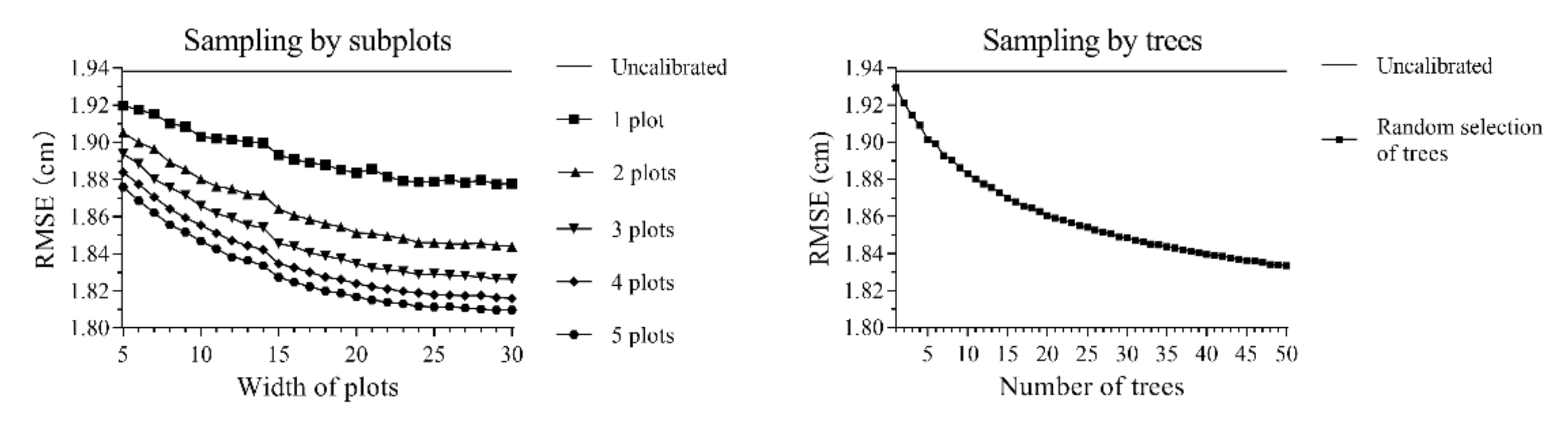
Random selection of 1‒50 individual sample trees across a validation site.

(2)

Random selection of 1‒5 square subsample plots with various sizes (length of 5‒30 m) within a validation site. Furthermore, all trees located in the subsample plots were selected for calibration.

2.5. Benchmarking with Nonparametric Models

Nonparametric modeling methods have been used to estimate forest attributes from LiDAR-derived data which involve fewer assumptions and could achieve higher prediction accuracy [36,74]. In the present study, the two most common nonparametric modeling methods (random forest and k-Nearest Neighbors) were applied for further comparison with the NLME models.

2.5.1. Random Forest

Random forest (RF) is a technique that creates a set of decision trees and then aggregates the results for classification and regression [75]. Each tree is generated independently using bootstrap samples from the training dataset called “in-bag samples” (usually two-thirds of the data). Meanwhile, the remaining “out-of-bag” (OOB) samples are used for internal cross-validation. The relative importance of each metric was ranked by quantifying the mean square error increase when each variable of the OOB samples is randomly permuted [75]. Depending on the variable importance ranking, an iterative backward elimination procedure is used for stepwise variable selection [76]. All the variables were first added in an RF, and the less important variable was eliminated; the variable importance was then recalculated using the remaining variables. This procedure was iteratively repeated until a given number of variables was obtained. Herein, 15 predictors were selected from all extracted variables for RF modeling since some additional variables could not significantly decrease the OOB error (mean square error of the OOB samples); see Supplementary Materials Figure S3. Two parameters in the RF modeling, $n_{tree}$ and $m_{try}$, were set as 400 and 1/3, respectively.

2.5.2. k-Nearest Neighbors

The k-Nearest Neighbors (k-NN) algorithm is a nonparametric estimation method based on the statistical difference between the predictor values and the reference samples. The nearest neighbors used for prediction have been widely applied and discussed for forest applications [77,78]. Variable selection strategies and parameter optimization methods for nearest neighbor imputation have been discussed in detail in [76,78]. In this study, the variables obtained from the RF method were also applied for the k-NN method, as in [76]. For the k-NN computation, the most similar neighbor (MSN) distance metric was used with a canonical correlation analysis based weighting matrix to choose the most similar neighbors [79]. The neighbor number was set to five.

2.6. Model Evaluation and Validation

The extrapolation and transferability of the DBH estimation (via the base, generalized, NLME, RF, and k-NN models) were assessed using the observed data from independent regions (outside the scope of the modeling data). The leave-one-out cross-validation (LOOCV) was employed to avoid overestimations [80,81]. In particular, we adapted the site-level LOOCV method (named leave-one-site-out cross-validations) instead of the commonly used tree- and plot-level. It was run by iteratively leaving out one site (N − 1) from the full dataset, aiming to simulate the estimations’ expansibility bias across different sites [39]. The mean error (BIAS, in cm) and root mean square error (RMSE, in cm) were computed using the predicted and observed DBH in the site-level LOOCV as follows:

$$\mathrm{BIAS}=\frac{{{\displaystyle \sum }}_{i=1}^m{{\displaystyle \sum }}_j^{n_i}\left(D_{ij}-{\widehat{D}}_{ij,-i}\right)}{{{\displaystyle \sum }}_{i=1}^m{n}_i},$$

(6)

$$\mathrm{RMSE}=\sqrt{\frac{{{\displaystyle \sum }}_{i=1}^m{{\displaystyle \sum }}_j^{n_i}{\left(D_{ij}-{\widehat{D}}_{ij,-i}\right)}^2}{{{\displaystyle \sum }}_{i=1}^m{n}_i}},$$

(7)

where $D_{ij}$ is the observed DBH value of the $j$th tree in the $i$th sample site; ${\widehat{D}}_{ij,-i}$ is the predicted value of the model, which was fitted using all observations without the $i$th sample site; $m$ is the number of sample sites; and $n_i$ is the number of observations in the $i$th sample sites. Simultaneously, relative BIAS and RMSE (BIAS% and RMSE%) were also applied for evaluation.

Both estimation types (with and without local calibration) were included for validating the NLME prediction. The single- or multivariable (base and generalized model in the NLME modeling) weighted nonlinear least square regression and nonparametric methods (RF and k-NN) were compared with the NLME model for DBH estimation.

3. Results

3.1. Model Fitting

The parameter estimates and fitting performances of the one-variable base model (Equation (1)), multivariable generalized model (Equation (3)) and NLME model (Equation (4)) are presented in

Table 2. Parameter estimates and fitting statistics for the base, generalized, and nonlinear mixed-effects (NLME) models.

	Parameter	Base	Generalized	NLME
Fixed Parameters	$a_0$ ($a$ in base model)	3.0560	2.8457	2.0063
	$a_1$		0.3337	0.3289
	$a_2$		0.0168	0.0198
	$a_3$		−0.1933	−0.1933
	$b$	0.3623	0.3848	0.5851
	$c$	0.0398	0.0235	0.0119
Variance parameters	${\sigma }_{u_0}^2$			0.0589
	${\sigma }_{u_1}^2$			0.0032
	${\sigma }_{u_3}^2$			0.0098
	${\sigma }_{u_0,u_1}$			−0.0094
	${\sigma }_{u_1,u_3}$			0.0007
	${\sigma }_{u_0,u_3}$			−0.0176
	${\sigma }^2$	0.3102	0.4199	0.6102
	$\mathsf{\gamma }$	0.5787	0.4049	0.3131
Fitting Statistics	$R_a^2$	0.8105	0.9026	0.9132
	RMSE	2.6397	1.8926	1.7872
	AIC	39,976.27	34,415.39	33,385.81
	LL	−19,986.13	−17,200.69	−16,678.90

. The base model described about 81% of variation while applying tree height as a sole predictor. After adding covariates ($CD$, $C{C}_{p75}$, and $Cn{p}_R$) into the univariable base model, there was a considerable enhancement in model fitting; the RMSE decreased by about 30% (from 2.6397 to 1.8926) and the $R_a^2$ increased by about 10% (from 0.8105 to 0.9026). Meanwhile, both the AIC and LL in Equation (3) had a 14% decrease and increase, respectively. These results show that the fitting performance of Equation (3) is more generalized than that of the base model. Furthermore, there was a further improvement in the model fitting after introducing site random effect parameters of $u_0$, $u_1$, and $u_5$; the NLME model achieved a higher $R_a^2$ and LL and a lower RMSE and AIC than the generalized model. In addition, the result of LRT between the generalized and NLME models was statistically significant (p < 0.0001), which implied that there were significant site-level random effects on the variation in DBH.

3.2. Evaluation and Comparison

3.2.1. Different Calibration for NLME Model

We applied two strategies (subplots’ and trees’ random sampling) to locally calibrate the NLME model and calculate the site-level random effects for predicting DBH. Both of the calibration methods were repeated continuously 1000 times. The average RMSE is presented in Figure 4. For each method, the subject-specific prediction with local calibrated random effects could achieve lower RMSE than the uncalibrated NLME model (mean response prediction by the fixed parameters presented in Table 2). The RMSE values decreased with the increasing number of sampling blocks and the width of blocks. In addition, the RMSE also decreased as the number of trees increased. Overall, the prediction accuracy has a positive correlation with the sampling number, indicating that more trees being used for estimating the random-effects parameters will yield a higher prediction accuracy. Considering the time and cost of the in situ measurements, we herein applied the feasible scheme of sampling 20 trees at a particular calibration site as a baseline for NLME prediction to compare with other methods.

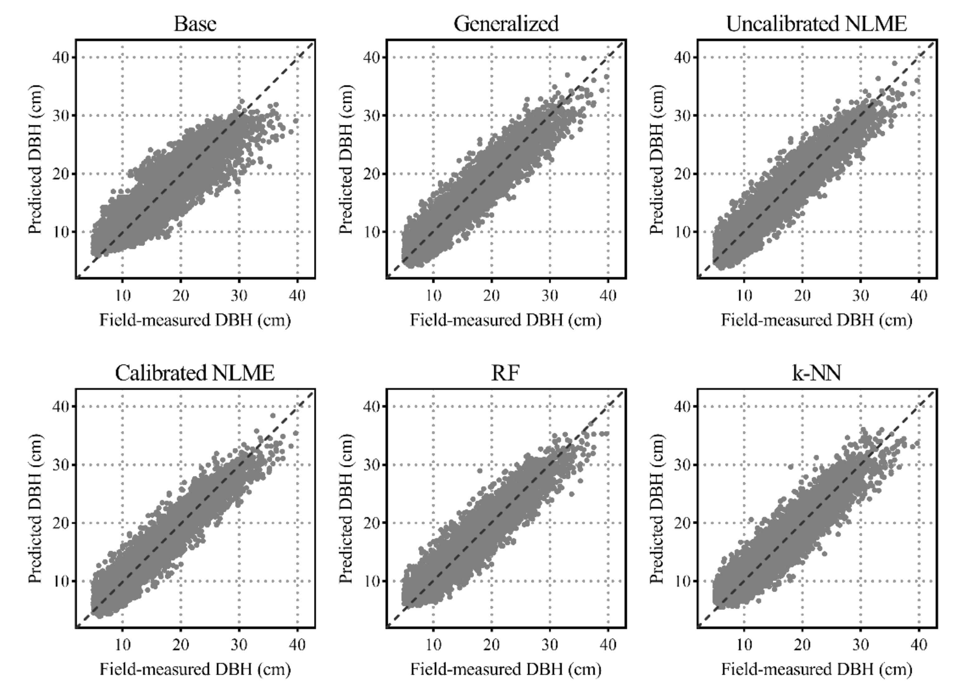
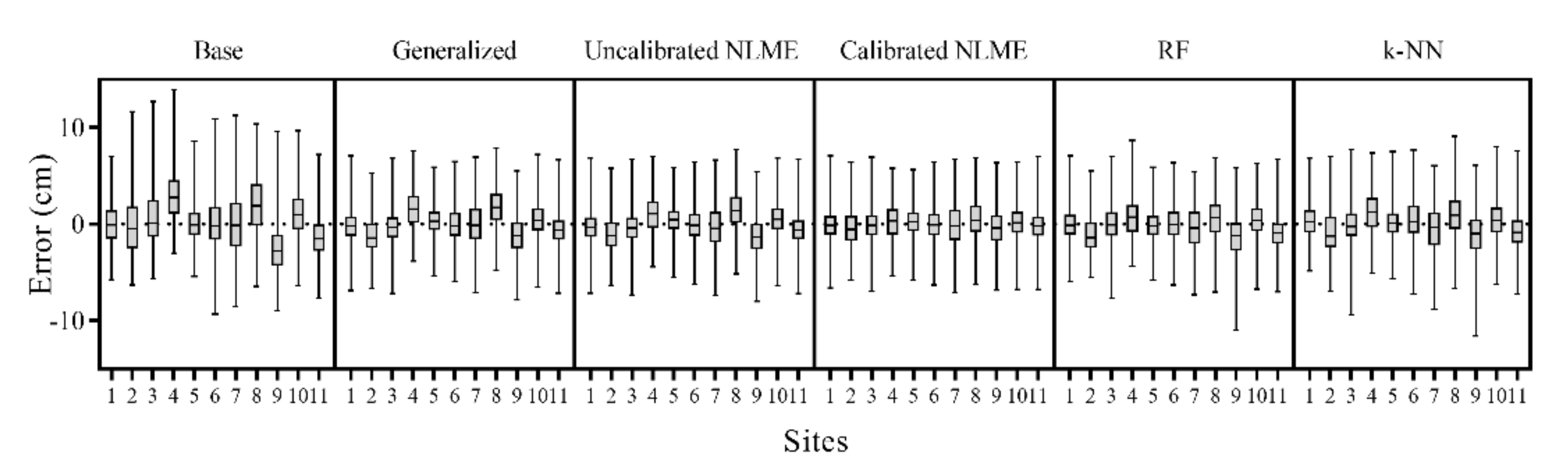
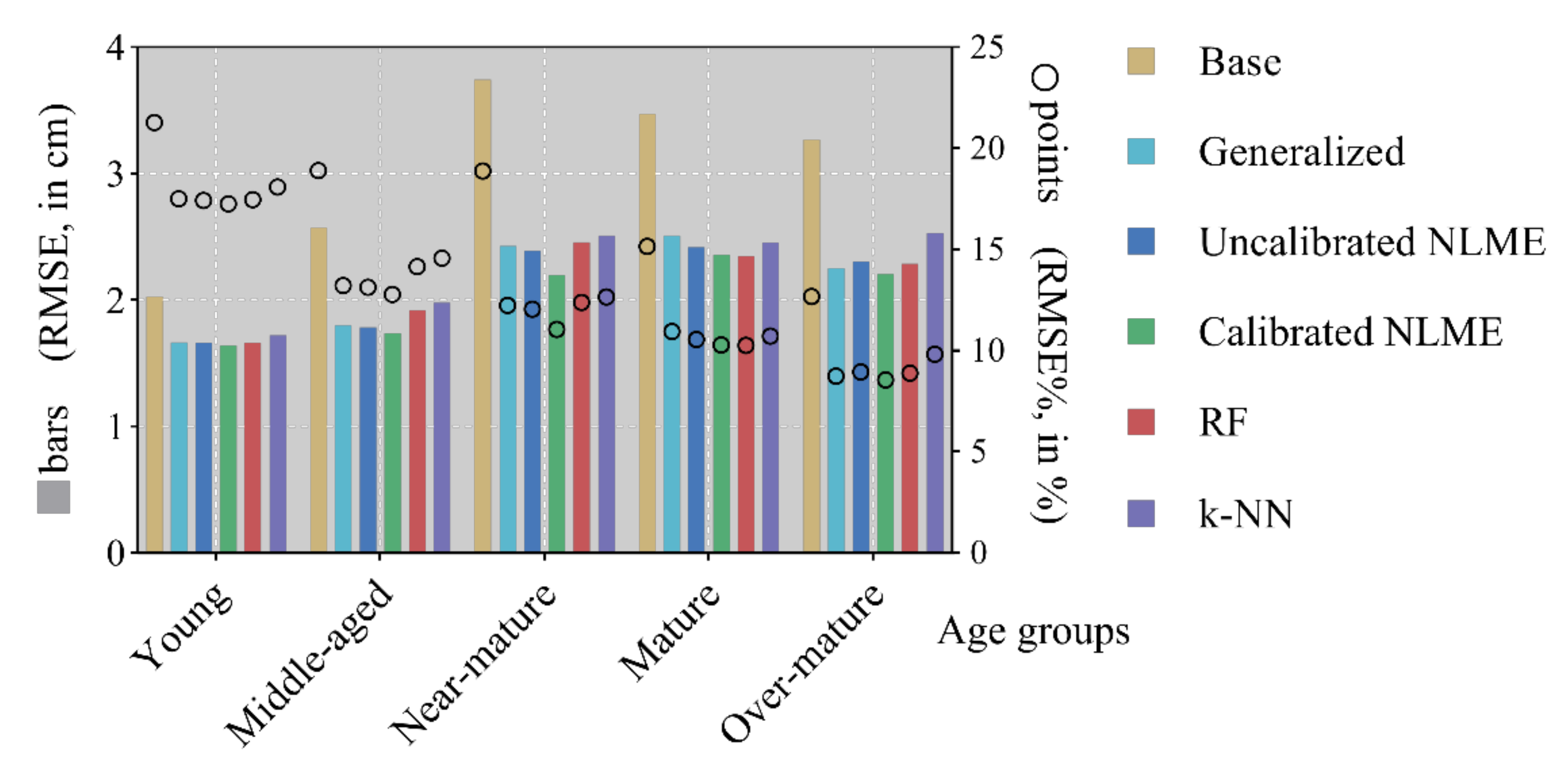
3.2.2. Comparison of Prediction

The results of the six DBH estimators are shown in

Table 3. Prediction accuracies of diameter at breast height (DBH) for the different models.

Model	BIAS (cm)	BIAS% (%)	RMSE (cm)	RMSE% (%)
Base	−0.14	−0.93	2.76	18.58
Generalized	−0.05	−0.36	1.96	13.17
Uncalibrated NLME	−0.08	−0.56	1.94	13.03
Calibrated NLME	0.02	0.10	1.86	12.51
RF	−0.28	−1.89	2.00	13.42
k-NN	−0.10	−0.67	2.08	13.97

and Figure 5. The base univariable model with the LiDAR-derived tree height data as the only predictor had a relatively poorer performance than the other multivariable equations. This indicated that using tree height as a sole predictor is insufficient to explain the variation in DBH. The NLME prediction calibrated with 20 sampling trees exhibited the lowest BIAS (0.02 cm) and RMSE (1.86 cm). Compared to the generalized model and the uncalibrated NLME model, the insertion of site-level random effects led to an improvement in the prediction accuracy. The generalized and uncalibrated model performed slightly better than the two nonparametric models (RF and k-NN). The accuracy assessments based on leave-one-site-out cross-validation showed the transferability of the multivariable parametric model across different sites. Figure 5 presents the relationship between the predicted and the field-measured diameter at breast height (DBH) calculated with six different methods, which shows that the calibrated NLME method has more compact and uniformly distributed points on both sides of the $y = x$ trend line.

The predictions across 11 different sites were separately assessed, and the RMSE values are given in

Table 4. The root mean square error (RMSE, in cm) of the six methods across the 11 sites.

Site	Base	Generalized	Uncalibrated NLME	Calibrated NLME	RF	k-NN
1	2.21	1.67	1.68	1.64	1.67	1.78
2	3.39	2.37	2.29	2.14	2.32	2.60
3	2.75	1.79	1.81	1.77	1.86	1.93
4	3.99	2.53	2.24	2.01	2.25	2.54
5	1.94	1.68	1.71	1.66	1.68	1.70
6	2.86	1.94	1.91	1.89	2.00	2.17
7	3.55	2.38	2.41	2.37	2.42	2.51
8	3.84	2.81	2.63	2.22	2.29	2.49
9	3.63	2.38	2.45	2.15	2.54	2.50
10	2.53	1.87	1.85	1.78	1.90	2.01
11	2.46	1.75	1.73	1.64	1.94	1.97

. The univariable base model always had the worst accuracy at every site, while the multivariable parametric and nonparametric models achieved more reliable results. Meanwhile, the NLME model with local calibration always achieved the highest prediction accuracy, with the RMSE values ranging from 1.64 to 2.37. Using 20 sample trees per site for local calibration might decrease the RMSE value by 0.02‒0.41 with respect to the uncalibrated prediction. The six models’ residuals were plotted across 11 sites in Figure 6. The error range of the calibrated NLME model was relatively stable compared with other methods across all 11 sites, which indicated a more stable prediction accuracy and better transferability between different sites. The calibrated NLME model indicates the robustness of the mixed-effects modeling technique, which is suitable when the predictor properties are highly varied. The mixed-effects model comprises both fixed- and random-effects parameters, which can express not only the mean response of the whole population but also the variation between individuals.

In addition, the prediction results of the six approaches were assessed across different forest structures (age groups). The RMSE and RMSE% values are plotted in Figure 7. The RMSE% values were the worst in young stands and decreased with the increase in age for all methods. The univariable base model always exhibited the worst performance, while the multivariable parametric and nonparametric models had substantial improvements in the RMSE and RMSE% values in each age group. Furthermore, the calibrated NLME model almost presented the best prediction accuracies across different age groups. The calibrated NLME model decreased the RMSE and RMSE% values by 1‒8% compared with the uncalibrated prediction and achieved the smallest improvement in young stands.

4. Discussion

In recent years, miniaturized laser scanning sensors on unmanned aerial vehicle platforms have gained an outstanding reputation in practical forest inventory [10,82,83]. Using remotely sensed data for individual tree DBH estimation is an appealing prospect, providing a new way to quantify the stand’s volume, biomass, and carbon stock and to reconstruct other forest attributes (e.g., stem diameter distributions [18,19,20]). To address the issue of DBH prediction from UAVLS data, herein we utilized a multi-echo RIEGL UVX1-mini sensor to scan 11 plantation sites of larch, one of the most abundant and economically important species in northeast China. We applied the NLME modeling approach to establish the generalized individual tree DBH equation. The accuracy of the developed equation was evaluated and compared with the weighted nonlinear least squares model and nonparametric regressions through leave-one-site-out cross-validation.

LiDAR-derived tree height data are often utilized to estimate DBH because of the robustness of the LiDAR-derived height measurements and the strong relationship between DBH and tree total height [21,22,63]. In this study, we also used tree height as a basic predictor for NLME modeling. The covariates and random effects were then introduced for model generalization. The results show that the base univariable model performed less well than the multivariable model. This finding corroborates previous research conducted by Jucker et al. (2017), which reported difficulties in using LiDAR-derived tree height data as a sole predictor to reflect the DBH variation [22]. Although some studies have achieved relatively a good performance and high accuracy, the diameter ranges and species information should be taken into account in developing the model for a proper comparison [21,60]. On most occasions, each species has a maximum growth limit of the tree height, and the relationship between DBH and tree height across various ranges of tree size is generally nonlinear [27,63]. The inclusion of crown attributes is essential in order to differentiate trees of a similar height with substantially different diameter sizes. Several crown attributes, such as crown project area, crown surface area, and crown volume, have been reported to have a significant influence on increasing the prediction accuracy of DBH [28,29,63]. In the present study, adding these crown attributes to the model did not lead to any significant improvement compared to using crown diameter.

The diameter growth of individual trees is also affected by the growing environment and stand conditions [30,31]. Hence, our study introduced the LiDAR-derived competition index ($C{C}_{p75}$) and plot-level metrics ($Cn{p}_R$) into DBH modeling. $C{C}_{p75}$ represents the competition status, which has a negative effect on DBH growth. $Cn{p}_R$ is the canopy rugosity within each plot, which could be considered as the explanation of the stand density and reflects the variation in the canopy surface’s height; the smaller the overlaps between crowns, the greater the variation. The proposed multivariable generalized model shows a high flexibility, which could further explain the DBH variation under similar height and crown sizes. In previous studies, Paris and Bruzzone (2019) also took topography metrics to improve the DBH estimation [24]. However, due to the small terrain difference in our study area, no particular topographical metrics were incorporated in the generalized model. The features selected for stepwise selection using the random forest nonparametric are the height, crown, and competition metrics of the individual tree- and plot-level canopy height metrics (Supplementary Material Figure S3), which emphasizes the importance of the abovementioned variables in describing the DBH variation. With respect to the comparison of predictions among different age groups, all the methods performed the worst in the young stand. This might be because height measurements were taken as the main predictor for DBH estimation, but DBH variation may not be explained well by tree height variation in young stands compared with other stands (see the RMSE% values of the base model in Figure 7). The DBH of larch grows fast at a young stage, so factors reflecting the tree’s vigor (such leaf area, site index) may be helpful and should be tried in studies focusing on young stands.

A lot of previous studies have applied nonparametric models to predict DBH utilizing LiDAR-derived variables [34,35]. In our studies, the benchmark from nonparametric models (RF and k-NN) had a relatively reliable performance (see Table 4). However, they still showed slightly higher RMSE values than both uncalibrated and calibrated NLME models in site-level LOOCV, which confirmed the advantage of the parametric model for extrapolating data outside the coverage of the model fitting data [36].

The inclusion of random-effects parameters led to a further improvement in both the model fitting and prediction. Specifically, the calibrated NLME prediction with a small number of resampling field measurements led to more stability and a better accuracy than other methods across all UAVLS-inventoried areas. Although using more variables can improve the generalization of the model, the site environmental variation and the uncertainty in the data acquirement process reduce the model transferability [39,57]. Many studies have attempted to analyze the transferability of airborne LiDAR-based models. Breidenbach et al. (2008) employed mixed-effects models across separate datasets. They found that the mixed-effects model (with both fixed and random effects) was able to more precisely predict DBH using stand attributes from two different inventory areas than the fixed-effects model [84]. Korhonen et al. (2019) applied an established mixed-effects model to other inventory areas outside the scope of the data used in the model’s development process [57]. Their results revealed that measuring a small number of calibration trees could decrease systematic errors, which increases the model’s transferability. The mixed-effects model includes both fixed and random effects parameters, and so can be adapted to a specific site. It can reflect not only the general trend of the sites but also the variation between individuals. The mixed-effect model’s transferability can be utilized to calibrate the models for further purposes, providing a new way to improve the model’s portability and ductility, especially for UAV-based small-scale forest applications.

Different from previous studies, which mainly applied plot-level mixed-effects models [57,63,85], in the current study we introduced a site-level NLME model to explain the site variability in the tree growth using both LiDAR point clouds and field data. Even after applying similar scanning and flight parameters, different UAVLS devices may produce remarkably different point clouds due to the various forest conditions [6,41]. For small-area forest inventories using UAV platforms, high-precision point clouds could obtain the individual tree information at a 1 km² coverage per scan, breaking the spatial limitation of traditional forest survey sample plots [14,86]. After establishing the models, site-level random effects can be directly and easily used to calibrate the entire UAV flight site, without needing to establish plot-level mixed-effects models for independent calibration. Although a higher prediction accuracy can be obtained by using a smaller scale of mixed effects, a shift from the sample plot survey to focus on the whole stand is needed when UAV is used for small-area forest surveys. The approach proposed in this study might provide a more affordable option for operational forestry.

Using an optimal number of sample trees in mixed-effects model calibration will deliver a relatively high prediction accuracy and appears to be a more efficient strategy for forest management [37,85]. Both of the sampling strategies (based on subplots and individual trees) behaved logically in relation to the amount of calibration information (Figure 4), as corroborated by previous studies on forest modeling [63,65,66]. In the field measurements, plot delineation often required extra labor compared to random tree sampling. As a result, when comparing the prediction accuracy (Section 3.2.2) we only selected 20 sample trees for local calibration, which is more realistic in the actual application. From the prediction results among different age groups, the calibration performance exhibits the lowest improvements in the young stand because the higher stand density in young forests leads to a lower calibration quantity. Proportional resampling methods may obtain more consistent improvements in forests with different densities, but increase the workload of high-density stands. Extending the sample quantity will improve the model’s accuracy in a linear correlation with the increasing inventory cost; thus, the optimum practical calibration approach should be determined based on a compromise between accuracy and efficiency [85].

From the perspective of practical applications, another problem that needs to be addressed is the impact of individual tree segmentation errors. It seems that there were relatively high commission errors in our study for larch plantations compared with others; this is mainly due to the fact that the segmentation methods was sensitive to the outer trees with their crowns extending into the plot boundaries, as shown in Figure 3. However, this indeed has few impacts on the subsequent parameter extraction and DBH modeling in our study, since we only used matched trees and the incomplete segmented crowns along plot boundaries were also excluded for model development. In practical application in forest inventory, commission and omission errors may lead to potential errors in the applications of established DBH estimation models [20]. In particular, segmentation errors and DBH estimation bias may cause error transfer from individual tree to plot-level forest parameter estimation such as stem diameter distribution and forest biomass estimation [18,19,87]. An edge-tree correction could have a significant contribution for the following individual as well as plot-level application of the developed models, as in [88] and [89]. On the other hand, many studies have revealed that stand densities and dominant positions may strongly affect the performance of individual tree delineation. More segmentation errors brought about greater challenges in DBH estimation for small trees and high-density young forests [90,91]. Together with the relatively poor prediction accuracy in young stands (Figure 7), it is necessary to further explore the proposed method for application in young trees. In addition, our study only proposed a species-specific DBH estimation modeling method. In practical applications, it is often necessary to classify tree species in the first step and then choose the modeling approach depending on the tree species, as in [55].

With the development of LiDAR technology, many studies have attempted to directly extract DBH from high-density UAV‒LiDAR point clouds. The previously published study of Wieser et al. (2017) focused on utilizing UAVLS point cloud data to estimate DBH from manually delineated tree stems during the leaf-off season in a deciduous forest [92]. Kuželka et al. (2020) applied an automatic diameter measurement and tree stem detection procedure in mixed Norway spruce and Scots pine forests with a stand density of less than 500 stems/ha; they achieved a relative RMSE value of 19% for DBH estimation [93]. Liang et al. (2019) compared the results of manual and automatic DBH measurements using UAVLS. The relative RMSE of automated and manual measurements was around 15‒30% with different stand complexities [86]. These studies implied that DBH direct measurements lacked robustness, as the performance was affected by the penetration of laser sensors and forest conditions [86]. Overall, we are looking forward to using direct extracted UAVLS point cloud DBH for calibration in future research, minimizing the burden of field measurement and model application.

5. Conclusions

This study introduces a framework for model-based individual tree diameter at breast height (DBH) estimation in UAVLS forest inventories. The tree- and plot-level LiDAR-derived metrics ($H$, $CD$,$C{C}_{p75}$, and $Cn{p}_R$) were found to be statistically significant, and hence were included in the DBH model development process. Although the selected variables improved the model’s generalization ability, there are still several unexplained sources of variation, which can be further described by adding the site-level random effects. The site-calibrated NLME model showed a more stable performance across different sites and achieved a higher prediction accuracy than other approaches, such as uncalibrated NLME, uni- or multivariable weighted nonlinear least square regression, and nonparametric regressions (random forest and k-nearest neighbors). Furthermore, the calibration led to logical behavior with respect to the amount of calibration information. The practitioners could realistically choose the sample sizes and calibration method according to the trade-off between the accuracy requirements and field-measurement costs. Utilizing site-level random effects improved the transferability of the LiDAR-based DBH estimation model, leading to a breakthrough in how we interact with forests in the future. The mixed-effect modeling approach is a flexible method and provides a foundation for UAVLS-based inventories in small-scale forests.

References

1. Pan, Y.; Birdsey, R.A.; Fang, J.; Houghton, R.; Kauppi, P.E.; Kurz, W.A.; Phillips, O.L.; Shvidenko, A.; Lewis, S.L.; Canadell, J.G.; et al. A Large and Persistent Carbon Sink in the World’s Forests. Science 2011, 333, 988–993. [Google Scholar] [CrossRef] [PubMed] [Green Version]
2. Forest Resources Assessment (FAO). Global Forest Resources Assessment 2015: How are the World’s Forests Changing? FAO: Rome, Italy, 2015. [Google Scholar]
3. White, J.C.; Wulder, M.A.; Varhola, A.; Vastaranta, M.; Coops, N.C.; Cook, B.D.; Pitt, D.; Woods, M. A Best Practices Guide for Generating Forest Inventory Attributes from Airborne Laser Scanning Data Using an Area-Based Approach; Natural Resources Canada: Victoria, BC, Canada, 2013. [Google Scholar]
4. Liang, X.; Hyyppä, J.; Kaartinen, H.; Lehtomäki, M.; Pyörälä, J.; Pfeifer, N.; Holopainen, M.; Brolly, G.; Francesco, P.; Hackenberg, J.; et al. International benchmarking of terrestrial laser scanning approaches for forest inventories. ISPRS J. Photogramm. Remote Sens. 2018, 144, 137–179. [Google Scholar] [CrossRef]
5. Tomppo, E.; Olsson, H.; Ståhl, G.; Nilsson, M.; Hagner, O.; Katila, M. Combining national forest inventory field plots and remote sensing data for forest databases. Remote Sens. Environ. 2008, 112, 1982–1999. [Google Scholar] [CrossRef]
6. Næsset, E. Predicting forest stand characteristics with airborne scanning laser using a practical two-stage procedure and field data. Remote Sens. Environ. 2002, 80, 88–99. [Google Scholar] [CrossRef]
7. Wulder, M.A.; White, J.C.; Nelson, R.F.; Næsset, E.; Ørka, H.O.; Coops, N.C.; Hilker, T.; Bater, C.W.; Gobakken, T. Lidar sampling for large-area forest characterization: A review. Remote Sens. Environ. 2012, 121, 196–209. [Google Scholar] [CrossRef] [Green Version]
8. Asner, G.P.; Mascaro, J. Mapping tropical forest carbon: Calibrating plot estimates to a simple LiDAR metric. Remote Sens. Environ. 2014, 140, 614–624. [Google Scholar] [CrossRef]
9. Zhen, Z.; Quackenbush, L.J.; Zhang, L. Trends in automatic individual tree crown detection and delineation-evolution of LiDAR data. Remote Sens. 2016, 8, 333. [Google Scholar] [CrossRef] [Green Version]
10. Yin, D.; Wang, L. Individual mangrove tree measurement using UAV-based LiDAR data: Possibilities and challenges. Remote Sens. Environ. 2019, 223, 34–49. [Google Scholar] [CrossRef]
11. Bhardwaj, A.; Sam, L.; Akanksha; Martín-Torres, F.J.; Kumar, R. UAVs as remote sensing platform in glaciology: Present applications and future prospects. Remote Sens. Environ. 2016, 175, 196–204. [Google Scholar] [CrossRef]
12. Kotivuori, E.; Kukkonen, M.; Mehtätalo, L.; Maltamo, M.; Korhonen, L.; Packalen, P. Forest inventories for small areas using drone imagery without in-situ field measurements. Remote Sens. Environ. 2020, 237, 111404. [Google Scholar] [CrossRef]
13. Guo, Q.; Su, Y.; Hu, T.; Zhao, X.; Wu, F.; Li, Y.; Liu, J.; Chen, L.; Xu, G.; Lin, G.; et al. An integrated UAV-borne lidar system for 3D habitat mapping in three forest ecosystems across China. Int. J. Remote Sens. 2017, 38, 2954–2972. [Google Scholar] [CrossRef]
14. Jaakkola, A.; Hyyppä, J.; Yu, X.; Kukko, A.; Kaartinen, H.; Liang, X.; Hyyppä, H.; Wang, Y. Autonomous collection of forest field reference—The outlook and a first step with UAV laser scanning. Remote Sens. 2017, 9, 785. [Google Scholar] [CrossRef] [Green Version]
15. Wallace, L.; Musk, R.; Lucieer, A. An assessment of the repeatability of automatic forest inventory metrics derived from UAV-borne laser scanning data. IEEE Trans. Geosci. Remote Sens. 2014, 52, 7160–7169. [Google Scholar] [CrossRef]
16. Wallace, L.; Lucieer, A.; Watson, C.S. Evaluating tree detection and segmentation routines on very high resolution UAV LiDAR ata. IEEE Trans. Geosci. Remote Sens. 2014, 52, 7619–7628. [Google Scholar] [CrossRef]
17. Quan, Y.; Li, M.; Zhen, Z.; Hao, Y.; Wang, B. The Feasibility of Modelling the Crown Profile of Larix olgensis Using Unmanned Aerial Vehicle Laser Scanning Data. Sensors 2020, 20, 5555. [Google Scholar] [CrossRef] [PubMed]
18. Xu, Q.; Hou, Z.; Maltamo, M.; Tokola, T. Calibration of area based diameter distribution with individual tree based diameter estimates using airborne laser scanning. ISPRS J. Photogramm. Remote Sens. 2014, 93, 65–75. [Google Scholar] [CrossRef]
19. Hou, Z.; Xu, Q.; Vauhkonen, J.; Maltamo, M.; Tokola, T. Species-specific combination and calibration between area-based and tree-based diameter distributions using airborne laser scanning. Can. J. For. Res. 2016, 46, 753–765. [Google Scholar] [CrossRef]
20. Xu, Q.; Li, B.; Maltamo, M.; Tokola, T.; Hou, Z. Predicting tree diameter using allometry described by non-parametric locally-estimated copulas from tree dimensions derived from airborne laser scanning. For. Ecol. Manag. 2019, 434, 205–212. [Google Scholar] [CrossRef]
21. Bi, H.; Fox, J.C.; Li, Y.; Lei, Y.; Pang, Y. Evaluation of nonlinear equations for predicting diameter from tree height. Can. J. For. Res. 2012, 42, 789–806. [Google Scholar] [CrossRef]
22. Jucker, T.; Caspersen, J.; Chave, J.; Antin, C.; Barbier, N.; Bongers, F.; Dalponte, M.; van Ewijk, K.Y.; Forrester, D.I.; Haeni, M.; et al. Allometric equations for integrating remote sensing imagery into forest monitoring programmes. Glob. Chang. Biol. 2017, 23, 177–190. [Google Scholar] [CrossRef]
23. Popescu, S.C. Estimating biomass of individual pine trees using airborne lidar. Biomass Bioenergy 2007, 31, 646–655. [Google Scholar] [CrossRef]
24. Paris, C.; Bruzzone, L. A Growth-Model-Driven Technique for Tree Stem Diameter Estimation by Using Airborne LiDAR Data. IEEE Trans. Geosci. Remote Sens. 2019, 57, 76–92. [Google Scholar] [CrossRef]
25. Lo, C.S.; Lin, C. Growth-competition-based stem diameter and volume modeling for tree-level forest inventory using airborne LiDAR data. IEEE Trans. Geosci. Remote Sens. 2013, 51, 2216–2226. [Google Scholar] [CrossRef]
26. Tao, S.; Guo, Q.; Li, L.; Xue, B.; Kelly, M.; Li, W.; Xu, G.; Su, Y. Airborne Lidar-derived volume metrics for aboveground biomass estimation: A comparative assessment for conifer stands. Agric. For. Meteorol. 2014, 198–199, 24–32. [Google Scholar] [CrossRef]
27. King, D.A. Linking tree form, allocation and growth with an allometrically explicit model. Ecol. Modell. 2005, 185, 77–91. [Google Scholar] [CrossRef]
28. Yao, W.; Krzystek, P.; Heurich, M. Tree species classification and estimation of stem volume and DBH based on single tree extraction by exploiting airborne full-waveform LiDAR data. Remote Sens. Environ. 2012, 123, 368–380. [Google Scholar] [CrossRef]
29. Chen, Q.; Gong, P.; Baldocchi, D.; Tian, Y.Q. Estimating basal area and stem volume for individual trees from lidar data. Photogramm. Eng. Remote Sens. 2007, 73, 1355–1365. [Google Scholar] [CrossRef] [Green Version]
30. Ma, Q.; Su, Y.; Tao, S.; Guo, Q. Quantifying individual tree growth and tree competition using bi-temporal airborne laser scanning data: A case study in the Sierra Nevada Mountains, California. Int. J. Digit. Earth 2018, 11, 485–503. [Google Scholar] [CrossRef]
31. Uzoh, F.C.C.; Oliver, W.W. Individual tree diameter increment model for managed even-aged stands of ponderosa pine throughout the western United States using a multilevel linear mixed effects model. For. Ecol. Manag. 2008, 256, 438–445. [Google Scholar] [CrossRef]
32. Pinheiro, J.C.; Bates, D.M. Mixed-Effects Models in S and S-PLUS; Springer: New York, NY, USA, 2000. [Google Scholar]
33. West, P.W.; Ratkowsky, D.; Davis, A. Problems of hypothesis testing of regeressions with multiple measurements from individual sampling units. For. Ecol. Manag. 1984, 7, 207–224. [Google Scholar] [CrossRef]
34. Vauhkonen, J.; Korpela, I.; Maltamo, M.; Tokola, T. Imputation of single-tree attributes using airborne laser scanning-based height, intensity, and alpha shape metrics. Remote Sens. Environ. 2010, 114, 1263–1276. [Google Scholar] [CrossRef]
35. Yu, X.; Hyyppä, J.; Vastaranta, M.; Holopainen, M.; Viitala, R. Predicting individual tree attributes from airborne laser point clouds based on the random forests technique. ISPRS J. Photogramm. Remote Sens. 2011, 66, 28–37. [Google Scholar] [CrossRef]
36. White, J.C.; Tompalski, P.; Vastaranta, M.; Saarinen, N.; Stepper, C. A Model Development and Application Guide for Generating an enhanced Forest Inventory Using Airborne Laser Scanning Data and an Area-Based Approach; Natural Resources Canada: Victoria, BC, Canada, 2017. [Google Scholar]
37. Hou, Z.; Mehtätalo, L.; McRoberts, R.E.; Ståhl, G.; Tokola, T.; Rana, P.; Siipilehto, J.; Xu, Q. Remote sensing-assisted data assimilation and simultaneous inference for forest inventory. Remote Sens. Environ. 2019, 234, 111431. [Google Scholar] [CrossRef]
38. Karjalainen, T.; Korhonen, L.; Packalen, P.; Maltamo, M. The transferability of airborne laser scanning based tree-level models between different inventory areas. Can. J. For. Res. 2019, 49, 228–236. [Google Scholar] [CrossRef] [Green Version]
39. Kotivuori, E.; Korhonen, L.; Packalen, P. Nationwide airborne laser scanning based models for volume, biomass and dominant height in Finland. Silva Fenn. 2016, 50, 1–28. [Google Scholar] [CrossRef] [Green Version]
40. Næsset, E. Effects of different sensors, flying altitudes, and pulse repetition frequencies on forest canopy metrics and biophysical stand properties derived from small-footprint airborne laser data. Remote Sens. Environ. 2009, 113, 148–159. [Google Scholar] [CrossRef]
41. Korpela, I.; Ørka, H.; Maltamo, M. LiDAR–Effects of Stand and Tree Parameters, Downsizing of Training Set, Intensity Normalization, and Sensor Type. Silva Fenn. 2010, 44, 319–339. [Google Scholar] [CrossRef] [Green Version]
42. Keränen, J.; Maltamo, M.; Packalen, P. Effect of flying altitude, scanning angle and scanning mode on the accuracy of ALS based forest inventory. Int. J. Appl. Earth Obs. Geoinf. 2016, 52, 349–360. [Google Scholar] [CrossRef]
43. Gao, H.; Bi, H.; Li, F. Modelling conifer crown profiles as nonlinear conditional quantiles: An example with planted Korean pine in northeast China. For. Ecol. Manag. 2017, 398, 101–115. [Google Scholar] [CrossRef]
44. Zhang, W.; Qi, J.; Wan, P.; Wang, H.; Xie, D.; Wang, X.; Yan, G. An easy-to-use airborne LiDAR data filtering method based on cloth simulation. Remote Sens. 2016, 8, 501. [Google Scholar] [CrossRef]
45. Guo, Q.; Li, W.; Yu, H.; Alvarez, O. Effects of topographie variability and lidar sampling density on several DEM interpolation methods. Photogramm. Eng. Remote Sens. 2010, 76, 701–712. [Google Scholar] [CrossRef] [Green Version]
46. Li, W.; Guo, Q.; Jakubowski, M.K.; Kelly, M. A new method for segmenting individual trees from the lidar point cloud. Photogramm. Eng. Remote Sens. 2012, 78, 75–84. [Google Scholar] [CrossRef] [Green Version]
47. Hao, Y.; Zhen, Z.; Li, F.; Zhao, Y. A graph-based progressive morphological filtering (GPMF) method for generating canopy height models using ALS data. Int. J. Appl. Earth Obs. Geoinf. 2019, 79, 84–96. [Google Scholar] [CrossRef]
48. Khosravipour, A.; Skidmore, A.K.; Isenburg, M.; Wang, T.; Hussin, Y.A. Generating pit-free canopy height models from airborne lidar. Photogramm. Eng. Remote Sens. 2014, 80, 863–872. [Google Scholar] [CrossRef]
49. Puliti, S.; Breidenbach, J.; Astrup, R. Estimation of Forest Growing Stock Volume with UAV Laser Scanning Data: Can It Be Done without Field Data? Remote Sens. 2020, 12, 1245. [Google Scholar] [CrossRef] [Green Version]
50. Corte, A.P.D.; Souza, D.V.; Rex, F.E.; Sanquetta, C.R.; Mohan, M.; Silva, C.A.; Zambrano, A.M.A.; Prata, G.; Alves de Almeida, D.R.; Trautenmüller, J.W.; et al. Forest inventory with high-density UAV-Lidar: Machine learning approaches for predicting individual tree attributes. Comput. Electron. Agric. 2020, 179, 105815. [Google Scholar] [CrossRef]
51. Khosravipour, A.; Skidmore, A.K.; Isenburg, M. Generating spike-free digital surface models using LiDAR raw point clouds: A new approach for forestry applications. Int. J. Appl. Earth Obs. Geoinf. 2016, 52, 104–114. [Google Scholar] [CrossRef]
52. Zhao, Y.; Hao, Y.; Zhen, Z.; Quan, Y. A Region-Based Hierarchical Cross-Section Analysis for Individual Tree Crown Delineation Using ALS Data. Remote Sens. 2017, 9, 1084. [Google Scholar] [CrossRef] [Green Version]
53. Zhao, K.; Suarez, J.C.; Garcia, M.; Hu, T.; Wang, C.; Londo, A. Utility of multitemporal lidar for forest and carbon monitoring: Tree growth, biomass dynamics, and carbon flux. Remote Sens. Environ. 2018, 204, 883–897. [Google Scholar] [CrossRef]
54. Amiri, N.; Polewski, P.; Heurich, M.; Krzystek, P.; Skidmore, A.K. Adaptive stopping criterion for top-down segmentation of ALS point clouds in temperate coniferous forests. ISPRS J. Photogramm. Remote Sens. 2018, 141, 265–274. [Google Scholar] [CrossRef]
55. Dalponte, M.; Coomes, D.A. Tree-centric mapping of forest carbon density from airborne laser scanning and hyperspectral data. Methods Ecol. Evol. 2016, 7, 1236–1245. [Google Scholar] [CrossRef] [PubMed] [Green Version]
56. Coomes, D.A.; Dalponte, M.; Jucker, T.; Asner, G.P.; Banin, L.F.; Burslem, D.F.R.P.; Lewis, S.L.; Nilus, R.; Phillips, O.L.; Phua, M.H.; et al. Area-based vs tree-centric approaches to mapping forest carbon in Southeast Asian forests from airborne laser scanning data. Remote Sens. Environ. 2017, 194, 77–88. [Google Scholar] [CrossRef] [Green Version]
57. Korhonen, L.; Repola, J.; Karjalainen, T.; Packalen, P.; Maltamo, M. Transferability and calibration of airborne laser scanning based mixed-effects models to estimate the attributes of sawlog-sized scots pines. Silva Fenn. 2019, 53, 1–18. [Google Scholar] [CrossRef] [Green Version]
58. Biging, G.S.; Dobbertin, M. Evaluation of competition indexes in individual tree growth models. For. Sci. 1995, 41, 360–377. [Google Scholar] [CrossRef]
59. Almeida, D.R.A.; Stark, S.C.; Chazdon, R.; Nelson, B.W.; Cesar, R.G.; Meli, P.; Gorgens, E.B.; Duarte, M.M.; Valbuena, R.; Moreno, V.S.; et al. The effectiveness of lidar remote sensing for monitoring forest cover attributes and landscape restoration. For. Ecol. Manag. 2019, 438, 34–43. [Google Scholar] [CrossRef]
60. Salas, C.; Ene, L.; Gregoire, T.G.; Næsset, E.; Gobakken, T. Modelling tree diameter from airborne laser scanning derived variables: A comparison of spatial statistical models. Remote Sens. Environ. 2010, 114, 1277–1285. [Google Scholar] [CrossRef]
61. Yao, W.; Krull, J.; Krzystek, P.; Heurich, M. Sensitivity analysis of 3D individual tree detection from LiDAR point clouds of temperate forests. Forests 2014, 5, 1122–1142. [Google Scholar] [CrossRef] [Green Version]
62. Sharma, R.P.; Bílek, L.; Vacek, Z.; Vacek, S. Modelling crown width–diameter relationship for Scots pine in the central Europe. Trees Struct. Funct. 2017, 31, 1875–1889. [Google Scholar] [CrossRef]
63. Fu, L.; Duan, G.; Ye, Q.; Meng, X.; Luo, P.; Sharma, R.P.; Sun, H.; Wang, G.; Liu, Q. Prediction of individual tree diameter using a nonlinear mixed-effects modeling approach and airborne LiDAR Data. Remote Sens. 2020, 12, 1066. [Google Scholar] [CrossRef] [Green Version]
64. Fu, L.; Sun, H.; Sharma, R.P.; Lei, Y.; Zhang, H.; Tang, S. Nonlinear mixed-effects crown width models for individual trees of Chinese fir (Cunninghamia lanceolata) in south-central China. For. Ecol. Manag. 2013, 302, 210–220. [Google Scholar] [CrossRef]
65. Fu, L.; Sharma, R.P.; Hao, K.; Tang, S. A generalized interregional nonlinear mixed-effects crown width model for Prince Rupprecht larch in northern China. For. Ecol. Manag. 2017, 389, 364–373. [Google Scholar] [CrossRef]
66. Xie, L.; Widagdo, F.R.A.; Dong, L.; Li, F. Modeling height-diameter relationships for mixed-species plantations of Fraxinus mandshurica rupr. and Larix olgensis henry in Northeastern China. Forests 2020, 11, 610. [Google Scholar] [CrossRef]
67. Sharma, R.P.; Vacek, Z.; Vacek, S.; Kučera, M. Modelling individual tree height–diameter relationships for multi-layered and multi-species forests in central Europe. Trees Struct. Funct. 2019, 33, 103–119. [Google Scholar] [CrossRef]
68. Pinheiro, J.; Bates, D.; DebRoy, S.; Sarkar, D. Nlme: Linear and Nonlinear Mixed Effects Models. Available online: https://cran.r-project.org/package=nlme (accessed on 8 October 2020).
69. Calama, R.; Montero, G. Multilevel Linear Mixed Model for Tree Diameter Increment in Stone Pine (Pinus pinea): A Calibrating Approach. Silva Fenn. 2005, 39, 37–54. [Google Scholar] [CrossRef] [Green Version]
70. Yang, Y.; Huang, S.; Meng, S.X.; Trincado, G.; Vanderschaaf, C.L. A multilevel individual tree basal area increment model for aspen in boreal mixedwood stands. Can. J. For. Res. 2009, 39, 2203–2214. [Google Scholar] [CrossRef]
71. Meng, S.X.; Huang, S. Improved calibration of nonlinear mixed-effects models demonstrated on a height growth function. For. Sci. 2009, 55, 238–248. [Google Scholar] [CrossRef]
72. de-Miguel, S.; Mehtätalo, L.; Shater, Z.; Kraid, B.; Pukkala, T. Evaluating marginal and conditional predictions of taper models in the absence of calibration data. Can. J. For. Res. 2012, 42, 1383–1394. [Google Scholar] [CrossRef]
73. Robinson, G.K. That BLUP is a good thing: The estimation of random effects. Stat. Sci. 1991, 6, 15–32. [Google Scholar] [CrossRef]
74. Brosofske, K.D.; Froese, R.E.; Falkowski, M.J.; Banskota, A. A review of methods for mapping and prediction of inventory attributes for operational forest management. For. Sci. 2014, 60, 733–756. [Google Scholar] [CrossRef]
75. Breiman, L. Random Forests. Mach. Learn. 2001, 45, 5–53. [Google Scholar] [CrossRef] [Green Version]
76. Packalén, P.; Temesgen, H.; Maltamo, M. Variable selection strategies for nearest neighbor imputation methods used in remote sensing based forest inventory. Can. J. Remote Sens. 2012, 38, 557–569. [Google Scholar] [CrossRef]
77. Chirici, G.; Mura, M.; McInerney, D.; Py, N.; Tomppo, E.O.; Waser, L.T.; Travaglini, D.; McRoberts, R.E. A meta-analysis and review of the literature on the k-Nearest Neighbors technique for forestry applications that use remotely sensed data. Remote Sens. Environ. 2016, 176, 282–294. [Google Scholar] [CrossRef]
78. McRoberts, R.E.; Næsset, E.; Gobakken, T. Optimizing the k-Nearest neighbors technique for estimating forest aboveground biomass using airborne laser scanning data. Remote Sens. Environ. 2015, 163, 13–22. [Google Scholar] [CrossRef]
79. Maltamo, M.; Packalén, P.; Suvanto, A.; Korhonen, K.T.; Mehtätalo, L.; Hyvönen, P. Combining ALS and NFI training data for forest management planning: A case study in Kuortane, Western Finland. Eur. J. For. Res. 2009, 128, 305–317. [Google Scholar] [CrossRef]
80. Dong, L.; Zhang, L.; Li, F. Developing two additive biomass equations for three coniferous plantation species in northeast China. Forests 2016, 7, 136. [Google Scholar] [CrossRef] [Green Version]
81. Dong, L.; Zhang, Y.; Zhang, Z.; Xie, L.; Li, F. Comparison of tree biomass modeling approaches for larch (Larix olgensis Henry) trees in Northeast China. Forests 2020, 11, 202. [Google Scholar] [CrossRef] [Green Version]
82. Brede, B.; Calders, K.; Lau, A.; Raumonen, P.; Bartholomeus, H.M.; Herold, M.; Kooistra, L. Non-destructive tree volume estimation through quantitative structure modelling: Comparing UAV laser scanning with terrestrial LIDAR. Remote Sens. Environ. 2019, 233, 111355. [Google Scholar] [CrossRef]
83. Almeida, D.R.A.; Broadbent, E.N.; Zambrano, A.M.A.; Wilkinson, B.E.; Ferreira, M.E.; Chazdon, R.; Meli, P.; Gorgens, E.B.; Silva, C.A.; Stark, S.C.; et al. Monitoring the structure of forest restoration plantations with a drone-lidar system. Int. J. Appl. Earth Obs. Geoinf. 2019, 79, 192–198. [Google Scholar] [CrossRef]
84. Breidenbach, J.; Kublin, E.; McGaughey, R.J.; Andersen, H.-E.; Reutebuch, S.E. Mixed-effects models for estimating stand volume by means of small footprint airborne laser scanner data. Photogramm. J. Finl. 2008, 21, 4–15. [Google Scholar]
85. Maltamo, M.; Mehtätalo, L.; Vauhkonen, J.; Packalén, P. Predicting and calibrating tree attributes by means of airborne laser scanning and field measurements. Can. J. For. Res. 2012, 42, 1896–1907. [Google Scholar] [CrossRef]
86. Liang, X.; Wang, Y.; Pyörälä, J.; Lehtomäki, M.; Yu, X.; Kaartinen, H.; Kukko, A.; Honkavaara, E.; Issaoui, A.E.I.; Nevalainen, O.; et al. Forest in situ observations using unmanned aerial vehicle as an alternative of terrestrial measurements. For. Ecosyst. 2019, 6, 20. [Google Scholar] [CrossRef] [Green Version]
87. Xu, Q.; Man, A.; Fredrickson, M.; Hou, Z.; Pitkänen, J.; Wing, B.; Ramirez, C.; Li, B.; Greenberg, J.A. Quantification of uncertainty in aboveground biomass estimates derived from small-footprint airborne LiDAR. Remote Sens. Environ. 2018, 216, 514–528. [Google Scholar] [CrossRef]
88. Packalen, P.; Strunk, J.L.; Pitkänen, J.A.; Temesgen, H.; Maltamo, M. Edge-Tree Correction for Predicting Forest Inventory Attributes Using Area-Based Approach With Airborne Laser Scanning. IEEE J. Sel. Top. Appl. Earth Obs. Remote Sens. 2015, 8, 1274–1280. [Google Scholar] [CrossRef]
89. Pascual, A. Using tree detection based on airborne laser scanning to improve forest inventory considering edge effects and the co-registration factor. Remote Sens. 2019, 11, 2675. [Google Scholar] [CrossRef] [Green Version]
90. Wang, Y.; Hyyppa, J.; Liang, X.; Kaartinen, H.; Yu, X.; Lindberg, E.; Holmgren, J.; Qin, Y.; Mallet, C.; Ferraz, A.; et al. International Benchmarking of the Individual Tree Detection Methods for Modeling 3-D Canopy Structure for Silviculture and Forest Ecology Using Airborne Laser Scanning. IEEE Trans. Geosci. Remote Sens. 2016, 54, 5011–5027. [Google Scholar] [CrossRef] [Green Version]
91. Vauhkonen, J.; Ene, L.; Gupta, S.; Heinzel, J.; Holmgren, J.; Pitkanen, J.; Solberg, S.; Wang, Y.; Weinacker, H.; Hauglin, K.M.; et al. Comparative testing of single-tree detection algorithms under different types of forest. Forestry 2012, 85, 27–40. [Google Scholar] [CrossRef] [Green Version]
92. Wieser, M.; Mandlburger, G.; Hollaus, M.; Otepka, J.; Glira, P.; Pfeifer, N. A case study of UAS borne laser scanning for measurement of tree stem diameter. Remote Sens. 2017, 9, 1154. [Google Scholar] [CrossRef] [Green Version]
93. Kuželka, K.; Slavík, M.; Surový, P. Very High Density Point Clouds from UAV Laser Scanning for Automatic Tree Stem Detection and Direct Diameter Measurement. Remote Sens. 2020, 12, 1236. [Google Scholar] [CrossRef] [Green Version]
Figure 1. The site locations in the study area (coordinate system: WGS 1984 UTM Zone 52N).
Remotesensing 13 00024 g001
Figure 2. The comparison of canopy height models generated by (A) traditional first-echoes interpolation and (B) a graph-based progressive morphological filtering method.
Remotesensing 13 00024 g002
Figure 3. Examples of tree-to-tree matching. (A) Young forests with a stand density of about 3000 stems/ha; (B) mature forests with a stand density of about 700 stems/ha.
Remotesensing 13 00024 g003
Figure 4. Root mean squared error (RMSE, in cm) for the uncalibrated prediction and local calibrated prediction of the nonlinear mixed-effects model with two sampling strategies (based on subplots and trees).
Remotesensing 13 00024 g004
Figure 5. The predicted vs. field-measured diameter at breast height (DBH) for 8364 correctly delineated trees calculated using six different methods.
Remotesensing 13 00024 g005
Figure 6. The boxplots of errors (cm) among different models and 11 sites.
Remotesensing 13 00024 g006
Figure 7. The root mean square error (RMSE) and relative RMSE (RMSE%) of the six methods across different age groups. The left axis represents RMSE (bars) in cm and the right axis represents the RMSE% (points) in percentage.
Remotesensing 13 00024 g007