1. Introduction
Australia was seriously affected by the fire events known as “Black Summer” during the 2019–2020 summer season [
1]. At least 46 million acres of land burnt [
2] and “fires near me” became Google’s most searched words in Australia during that fire season [
3]. This fire disaster has raised a vital question regarding to what extent the wildfires’ occurrence can be linked to various climate, environmental, and social factors.
Nowadays, wildfire disaster risks are being heightened globally due to climate changes. High temperatures and prolonged dry seasons might result in unprecedented bushfire activities globally [
4]. The state temperature dataset, originating in 1910, reveals that Australia’s warmest year on record was in 2019, with the annual national mean temperature 1.52 °C above average. Australia’s climate in 2019 was the driest year on record, with significant heatwaves in January and December [
5]. However, human activities might be predominant rather than natural phenomena in wildfire ignition, as a recent study showed in Portugal [
6]. In this study, most wildfires were most likely triggered by human activities, as spatial patterns of wildfire ignition were strongly linked with human access to the natural landscape, with the proximity to urban areas and roads found to be the most important contributory factors. In respect to environmental and topography variables, the study conducted for the Mediterranean region showed that these variables were the main driving factors [
7]. The meteorological variables were strongly linked to the wildfires events in the U.S., especially in the West Coast over decades, where storms with lighting strike initially triggered a large number of fires and air temperature, drought, and wind leveraged fires to extreme burning [
8].
Satellite remote sensing has become a common tool for large-scale monitoring of ecosystems as well as spotting threats, e.g., wildfires, across the globe [
9]. Multiple studies have been already conducted using remote sensing and applied various approaches, such as kernel logistic regression or spatial logistic regression [
10,
11]. However, recently, machine learning (ML) approaches have rapidly progressed and achieved promising results in the environmental sciences [
12].
Significant studies have quantified the influence of natural and anthropogenic drivers of wildland fire ignitions with ML approaches [
13,
14,
15,
16] but they were conducted at regional–national level and without generating their own dataset of geographical location of fire occurrences. Thus, this study implemented an approach for generating a dataset including areas of previous fire occurrences at the continental level, i.e., the study site of Australia, and to train a model that observes the link between fire-conditioning factors and determines those that contribute to wildfires. This approach uses multiple state-of-the-art, openly available, satellite datasets and ML to obtain precise fire locations obtained from the Fire Information for Resource Management System (FIRMS) dataset and Sentinel-2 mission and reveal high-risk fire-prone landscape zones at the continental level. The study directly compared ML methods, including Random Forest (RF), Naïve Bayes (NB), and Classification and Regression Tree (CART) for wildfire mapping, and subsequently, a method with the best achieved performance in both model training and validation was used for mapping the wildfire susceptibility in Australia. Moreover, this study aimed to explore a set of causal variables, i.e., predictor variables, and to identify the dominant factors behind the recent wildfires in Australia. Modelling many complex environmental and socio-economic independent variables is often a difficult task due to large resource requirements, i.e., complexity as well as heterogeneous data formats. In that respect, most predictor variables, e.g., temperature, precipitation, population, etc., were gathered from the Google Earth Engine (GEE) data catalogue.
A training dataset in ML algorithms is an essential input supporting the model’s ability to learn [
17]. The process of generating a training dataset for supervised learning is frequently manual. Due to the extensive area and wide timeframe of the fire season, it is crucial to create an automated process for generating the most representative dataset for model training. Therefore, this study proposes an extensive automated workflow for generating a large training dataset across the entire Australia.
The wildfire challenges are related to some of the Sustainable Development Goals adopted in 2015 by the United nations with the aim to balance the economic, environmental, and social needs [
18]. The rising enhancement of geographic information technologies help to achieve the Sustainable Development Goals in many ways. Firstly, goal number 3 (Good Health and Well-being) as wildfire smoke contributes to air pollution and irritates the human respiratory system. Secondly, goal number 13, namely Climate Action, is considered due to the emitting carbon dioxide from wildfires along with other greenhouse gasses which accelerate global warming. Lastly, the goal 15 presents Life on Land, which is referred to by a massive impact of wildfires on land, which can lead to a short-term economic decline.
2. Materials and Methods
2.1. Study Area
The study area was the Australian mainland where the wildfires occurred over the 2019–2020 fire season. The Australian mainland includes five states, i.e., New South Wales, Queensland, South Australia, Victoria, Western Australia and major mainland territories, the Australian Capital Territory, and the Northern Territory. The map showing the area of interest is presented in
Figure 1. Australia, with a heavily concentrated population along the eastern and southeastern coasts, has a wide variety of landscapes, ranging from snow-capped mountains to large deserts. The eastern part of Australia is one of the most fire-prone areas in the world [
19].
The previously undertaken wildfire studies were not conducted on a state level due to the lack of computing power or absence of seamless datasets over the entire Australia. Thanks to the remarkable spatial and image-based analysis of GEE as well as its multi-petabyte of satellite images, it is possible to perform such a large scale and seamless analysis.
2.2. Exploratory Data Analysis—Active Fires
This section presents the exploratory analysis of Australian fires in the 2019–2020 season and compares them with the wildfires from the previous years to outline the main characteristics. The employed datasets for exploratory data analysis include different satellite missions, e.g., VIIRS, MODIS, which collect data regularly across the globe.
To perform this analysis, the European Center for Medium-Range Weather Forecast Reanalysis (ERA5) dataset was used. This dataset is freely available and offers a detailed overview of the atmosphere. The dataset covers the Earth on a 30 km grid and the atmosphere is divided into 137 levels from the surface up to a height of 80 km. This advanced product was released by The European Center for Medium-Range Weather Forecasts (ECMWF) [
20]. The ERA5 is part of GEE’s datasets consisting of air temperature band as a monthly average at 2 m height with availability from 1979 to present.
Figure 2 presents the mean annual temperature across Australia from 1979 to 2019. As can be seen, the mean annual temperature during these 40 years was the highest in 2019. The difference between the lowest mean annual temperature measured in 2000 and the highest measured in 2019 is approximately 1.8 °C. It is also important to note the highest mean temperature record was broken three times during the last two decades, in 2005, 2013, and 2019. This might suggest that Australia is becoming an increasingly warmer place, which is most likely a direct impact of global warming [
21].
For calculation of the total fire occurrences, the GEE’s Fire Information for Resource Management System (FIRMS) dataset was used. FIRMS distribute satellite-derived near real-time data within 3 h of satellite observation. FIRMS is part of NASA’s Land, Atmosphere Near real-time Capability (LANCE) for EOS and provides both the Moderate Resolution Imaging Spectroradiometer (MODIS) with Terra and Aqua EOS and the Visible Infrared Imaging Radiometer Suite (VIIRS) data [
22].
The active fires shown in
Figure 3 and
Figure 4 are presented as pixels covering 1 km
2 on the ground. Therefore, this pixel may contain one or more fire locations within a 500 m radius. Furthermore, the minimum detectable fire size depends on many variables, e.g., scan angle, land surface temperature, amount of smoke, etc. Generally, MODIS can detect both flaming and smoldering fires over 1000 m
2 size, but under extremely clean observing conditions smaller flaming fires can be detected (50 m
2) [
22]. Besides, the thermal anomalies, e.g., human activities, factories, and volcanoes, can be identified as active fires. The FIRMS dataset includes active fire locations via the pixel value, which determines the temperature of the surface in terms of Kelvin [
23].
Figure 3 presents the total number of pixels presenting the active fires in Australia each year from 2001 to 2019. The last year, 2019, compared to the previous 18 years does not present outstanding numbers. Both 2011 and 2012 stand for the worst years in terms of fire activity. Recorded active fires in 2017 and 2018 had both approximately 200,000 fires more than in 2019.
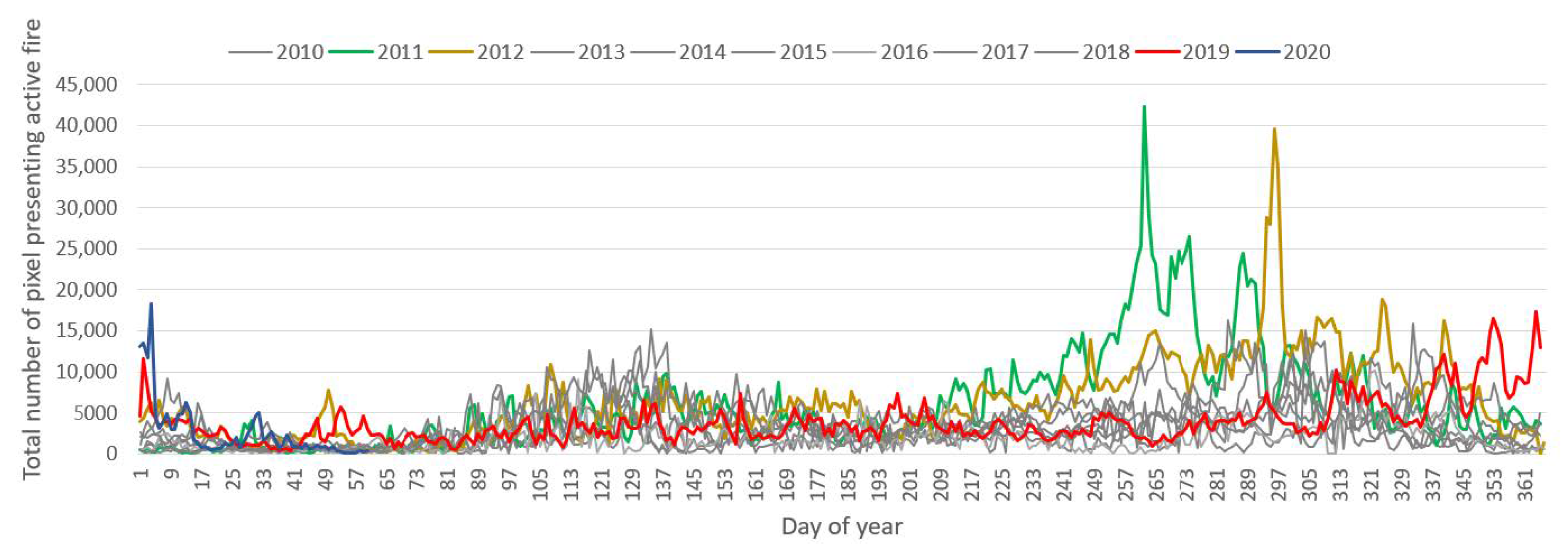
The detailed overview showing the fire activity over a year is required to uncover anomalies over months. Thus,
Figure 4 shows active fires over a year from 2010 to March 2020 in Australia. The 2011 and 2012 years had a significant number of active fires compared to other years. However, the satellite-driven fire data revealed that the most active fires during December and January throughout the last decade happened in 2019 and 2020, respectively. MODIS recorded about 400,000 active fire indicators over Australia between December 2019 and February 2020.
Figure 5 shows a spatial distribution map of active fire locations from January 2019 to February 2020. The shown fire locations were remarkably occurring in the north and east coast of Australia, while the south and west Australia witnessed slightly fewer fire events. The inland territory was less affected than the coastal area.
2.3. Methods
The following section describes the methodology used for fulfilling the two main objectives of this study. The entire structure is divided into three parts: (a) data mining and preprocessing, (b) classification, and (c) validation. This structure is presented in the flowchart in
Figure 6 and was intended to summarize the essential processes employed in this study.
The first step of the flowchart is creating the training dataset consisting of the historical fire events (as dependent variable) and the four main driver factors, including topographic, meteorological, anthropological, and vegetation factors (as independent variables). Subsequently, the historical fire events dataset was divided into training and testing datasets. The training dataset is applied in the ML models to train the model and then the trained model is validated by the testing dataset. The best performance from the selected ML models is used for the spatial prediction of wildfire susceptibility.
In this study, the Sentinel-2 mission was used to detect burnt areas using Normalized Burn Ratio (NBR). Overall, the difference between the spectral response of healthy vegetation and burnt areas reach their peak in the NIR and the SWIR regions of the spectrum. The NBR formula combines the near and short infrared wavelength [
24].
A higher difference of
NBR, calculated as
indicates more severely damaged areas, while areas with negative values may indicate the recovery following a fire event [
25].
proposed for mapping the burnt severity, relied on multispectral images, where
values could be interpreted based on the United States Geological Survey (USGS) [
24].
2.3.1. Data Mining and Preprocessing
The training dataset consisted of independent variables, also referred to as the predictors, and a dependent variable, also known as respond variable. In this study, the area of interest was at the continental level and the timeframe covered six months, thus leading to an overwhelming amount of data. Therefore, it was important to automate the process of generating the training dataset. This also brought a benefit of feeding the selected models with more samples of training data to improve the models’ performance.
2.3.2. Dependent Variable
The dependent variable in this study was the binary variable of
fire and
non-fire occurrence locations. Thus, mapping susceptibility of fire occurrence can be considered from the ML perspective as a binary classification problem with two classes: fire and no-fire. However, the dataset of recently occurred fire locations with high resolution was not available from the Australian official sources. Therefore, collecting fire and no-fire occurrence locations was developed in this study as an automated workflow, presented in
Figure 7.
This automated workflow was applied to each month of the fire season and changes in vegetation, e.g., bloom and harvest, might have biased the output results. The automated workflow used FIRMS dataset and Sentinel-2 mission, which were preprocessed in the interest of obtaining the fire occurrence locations. The FIRMS image collections aggregated active fire locations over the period of one month from the daily observations across Australia, with a 1 km2 employed bounding box. Subsequently, the areas of FIRMS fire locations were vectorized.
The Sentinel-2 data were employed in the second step due to its relatively fine spatial resolution. This mission produces cloud and cirrus masks created as a product of the atmospheric correction. These masks were applied with the aim to provide cloudless images and avoid misleading results in the analyses of the surface. A cloud mask band was already created in the Sentinel 2 L1C product and was generated based on the Band 2, Band 11, and Band 13; however, the cloud mask could be low, especially under critical atmospheric conditions. Subsequently, the Normalized Difference Water Index (NDWI) was computed using the Equation (3):
and was applied to remove the water areas from the analysis [
26]. The next step was to compute ΔNBR. The pre-fire NBR was calculated from an image collection with the time interval <6 days before the start of the month, start month> and post-fire NBR was determined from an image collection with the time interval <end month, 6 days after month>. The time interval should solve a problem with the unavailability of satellite data because the Sentinel-2 has a temporal period of 5 days. The ΔNBR calculation highlights the burnt areas and gets an initial assessment of burn severity. However, there is a ΔNBR obstruction, referring to a change detection process. This means that changes in natural vegetation [
27], e.g., deforestation and harvest, may be included as well. In other words, non-fire-related changes can be detected as wildfire damage. Despite the short-implemented period (one month), a ΔNBR threshold value of 0.44 was set up. This threshold selects the moderate–high severity or high severity burnt area and removes the unburned and low severity burn areas. The threshold was applied only within active fire vector areas from the FIRMS dataset. The aim was to eliminate the small natural vegetation changes and increase the computational power, as the calculation was performed inside the FIRMS fire vector areas. The combination of both features, burnt and fire areas, was applied for creating the balance as the burnt areas tend to underestimate the results, while active fire data may overestimate the results. The selected burnt areas inside the fire location boundary boxes were vectorized and afterwards, the sizes of selected burnt areas were calculated. The areas bigger than 0.25 km
2 (500 m × 500 m raster) were selected for generating the random points. The minimum size criteria means that the random points are in selected larger areas, as they represent a pixel which covers this particular area.
The no-fire point selection was performed using a random point function, where points are randomly placed outside of the FIRMS vector areas.
Figure 8 presents an example of one wildfire that occurred in September 2019 close to the West Coast of Australia. This figure presents the step-by-step results from the previously described processing.
The random point function used in the processing places randomly generated 300 fire points and 300 no-fire points for each selected part (each part contained 3 areas of Australia) for each month (from start of fire season in September 2019 and end of the fire season January 2020), which resulted in 18 CSV files consisting of 600 points per each file. These CSV files were merged into the final file using the JavaScript code. Each fire and no-fire record in the final file had the “Fire” property name and stored value in the integer type, where 1 represents a fire occurrence and 0 presents a no-fire occurrence.
2.3.3. Independent Variables
Selecting independent variables, which are also known as predictors or conditioning factors, is a critical step in predictive modelling. For this study, 15 conditioning factors were selected based on both the field observation found in different studies [
6,
7,
8,
28,
29] and available satellite data on the GEE platform. These applied wildfire conditioning factors could be divided into five categories, such as topography, vegetation type, infrastructure, meteorology, and socioeconomic factors.
Table 1 summarizes each of the datasets used in this study. GEE’s public data archive was used as the source data for the independent variables, except road network and electric lines. These data were imported directly as a raster data format and the links to data source to Earth Engine data catalogue are provided in the Source of Data column in
Table 1.
Topographic category (
Figure 9) consists of elevation, slope, and aspect. The elevation was obtained from the digital elevation model (DEM) with 30 m spatial resolution. The model was generated from the dataset gathered from the Shuttle Radar Topography Mission (SRTM) provided by NASA [
30]. The slope or the gradient of the land expressed as an angle and aspect, also known as the direction in which the slope faces, were derived from DEM.
Environmental category (
Figure 10) includes the land cover, soil depth, the soil moisture, the drought severity index, and the Normalized Difference Vegetation Index (NDVI). The Copernicus Global Land Service (CGLS) provided the evaluation of land cover at 100 m spatial resolution for the 2015 reference year [
31]. The dataset was derived from the 5 daily PROBA-V 100 m time-series with ground sampling, a database of high-quality land cover training sites and several ancillary datasets. The methodology covers the preprocessing of Earth Observation satellite (PROBA-V) observations, the calculation of metrics, the main classification, the regression for the versatile cover fraction layers, the time series break detection. The final product provides a primary land cover scheme with 23 classes in raster format with reaching an accuracy of 80%, where the forest, bare, and sparse vegetation classes are mapped with higher accuracies than shrubs and wetland classes. This offers sufficient accuracy and consistency in the land cover map [
32].
The soil depth gathered from the comprehensive Soil and Landscape Grid of Australia dataset describes the spatial distribution of the soil depth. The dataset includes outcomes from three-dimensional spatial modelling and combines historical soil data and estimates derived from visible and infrared soil spectra [
33].
The soil moisture raster and drought severity index were obtained from the Terra Climate 2019 dataset. This monthly dataset for global terrestrial surfaces uses the interpolated time-varying anomalies from CRU Ts 4.0/JRA55 with high-spatial climatological norms obtained from WorldClim dataset. Additionally, to produce monthly surface water balance, datasets apply a water balance model that incorporates reference evapotranspiration, precipitation, temperature, and interpolated plant extractable soil water capacity [
34]. These rasters were generated from the image collection obtained from September 2019 to December 2019, where the mean statistic function was implemented. This function takes the mean value of a given pixel over the period. Ideally, the final rasters of both variables should be calculated for the entire fire season; however, the Terra Climate is available only for the 2019 year.
The MOD13Q1 raster product directly provides the vegetation layer, i.e., NDVI, with the 250 m spatial resolution [
35]. The NDVI image was generated from the image collection collected during the entire fire season using the mean statistic function value.
Climate category (
Figure 11) includes mean values of precipitation accumulation, mean maximum temperature, and wind speed. These variables were gathered from the Terra Climate dataset and were processed in the same manner, i.e., collection obtained from September 2019 to December 2019, where the mean statistic function was implemented.
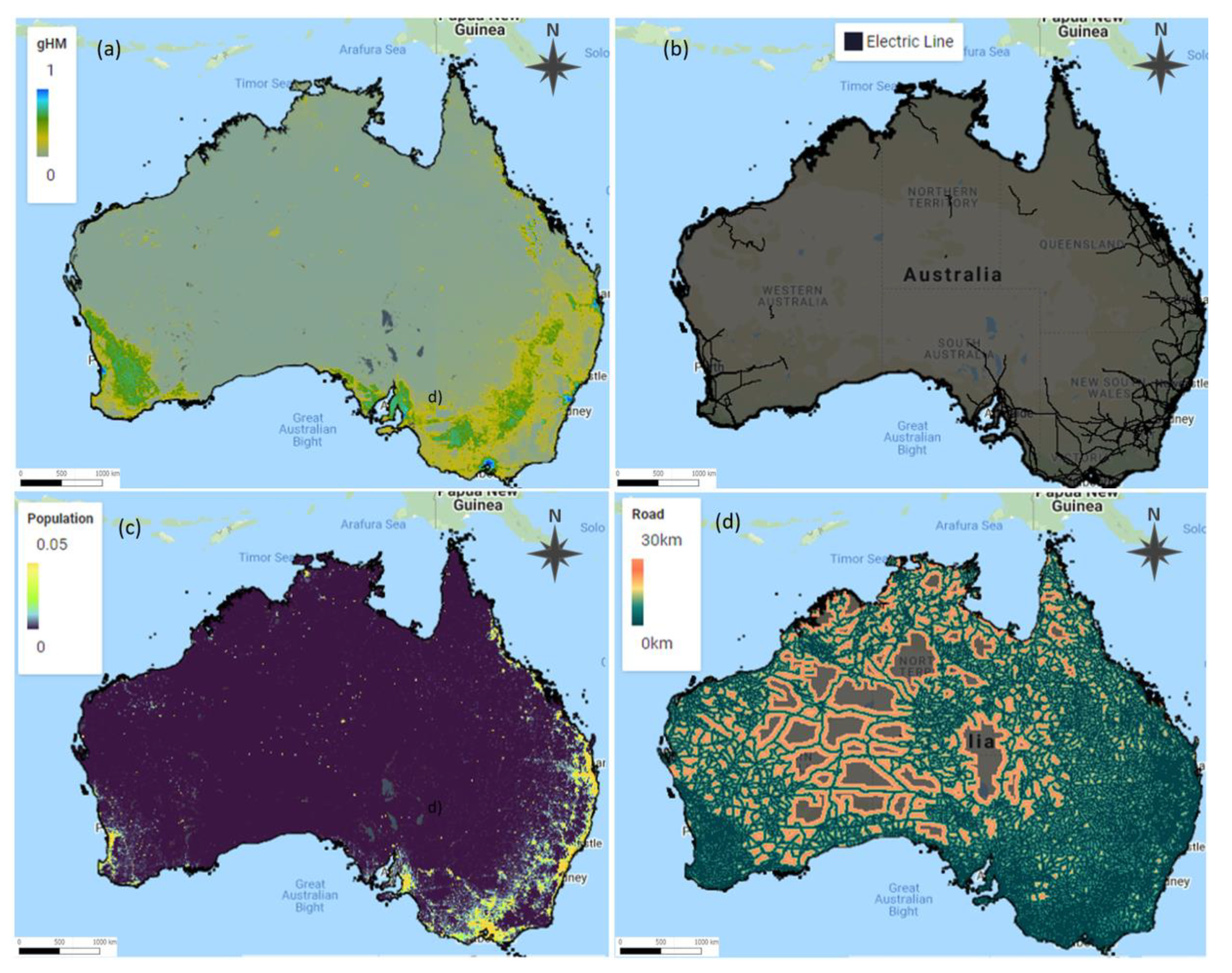
Socioeconomic category (
Figure 12) includes the Global Human Modification (GHM), population, electric lines, and distance from roads. The GHM dataset delivers a cumulative measure of human modification of terrestrial lands over the globe with 1 km spatial resolution. The GHM values vary from 0 to 1 and are associated with a given type of human modification, also known as a stressor. The major anthropogenic stressors are included, e.g., human settlement, transportation, mining, and energy production. The population from the WorldPop dataset estimated number of people residing in ≈85 m grid cells. The vector data, the electric lines, and road network were obtained from the Open Street Map (OSM) and converted to the raster format with 500 m resolution, where for the road distance, the GEE’s cumulative coast function was applied.
2.4. Classification
When the fire and no-fire training points were created and conditional factors preprocessed, the next step was to create the training dataset, which is enriched by predictor variables. Firstly, the 15 independent variables were merged to create a composite image with 15 bands. Afterwards, the SampleRegions function was applied to get the value of predictors into the table and generate training samples. Thus, the fire and no fire points were overlaid by the composite image to get predictor variables along with labels. A nominal scale for sampling is 100 m.
Once the training set was created, the next step was to evaluate the classification accuracy. The supervised pixel-based classifications rely heavily on the input training samples. Additionally, the GEE classifiers still have the limitation of not analyzing the variable importance. Even though this study compared three ML algorithms, only one model, specifically RF, can observe the link between fire conditioning factors and the fire occurrence, i.e., variable importance. Moreover, only the RF classifier in GEE provides the probability function [
36].
2.5. Validation
The trained ML models can predict the fire location; however, it is important to evaluate the performance of these models. For this reason, the accuracy assessment was conducted. The sample dataset of fire and no-fire location was divided into training and test datasets for model validation. This was conducted by applying the randomColumn function, which adds a column to the sample dataset and values into a column by default. The points were split with a ratio of 70:30 for training and testing, respectively. The accuracy assessment was applied to the testing dataset, which assessed accuracy based on the confusion matrix. From the confusion matrix, the overall accuracy and the kappa were derived.
3. Results
This section summarizes the findings of this study based on the applied methodology. The first section provides the results of the fire occurrence locations gathered from the Sentinel-2 mission and the FIRMS dataset. The second part of this section reveals the achieved results from the different ML algorithms, where employed prediction variables were gathered from the Earth observation, except for soil depth, the roads, and electric network data. The result of ML algorithms, the fire probability map, is presented in the third subchapter of this chapter. Finally, the last subchapter provides the results of the variable importance analysis, where results were derived from the ML algorithm.
3.1. Fire Occurrence Location
The fire occurrence points represent a location of individual fires that occurred during the fire season 2019–2020. The flowchart presented in
Figure 7 identifies the fire locations with 10 m accuracy automatically for the ML algorithms. The results show the distribution of fire and no-fire points locations and they are presented in
Figure 13. All these locations were a part of the sample training dataset, comprising of 10,800 training points across the Australian mainland.
The fire locations were visually verified from active fire alerts calculated from the Sentinel-2 data, as this can successfully recognize thermal trends [
37]. The highlighted hot spots were calculated using short-wave infrared (SWIR- Band 12) with near infrared wavelengths (NIR- Band 5) and stress burned areas and a wider range of short-wave infrared wavelengths providing more purified hotspot detection [
38]. The visualization of wildfire is based on the publicly available script from Sentinel Hub EO Browser. A simple color composite of bands SWIR/NIR/Red gives a sight of burnt areas but also highlights ongoing fire areas.
Figure 14 presents an example of the verification of fire points. Firstly, the pre-fire and post-fire area is visualized in the RGB image.
3.2. Accuracy Assessment of ML Algorithms
The widely used accuracy assessment method [
15,
39] was used to evaluate the performance of the ML models. Accuracy assessment gives a general understanding of how the model performs, therefore, the results of selected ML models were validated based on the accuracy assessment characteristics, i.e., confusion matrix, overall accuracy, and kappa statistics. The confusion matrix is a summary of prediction results on a classification where the number of correct and incorrect predictions are summarized with count values and broken down by each class. Overall accuracy is defined as the percentage of correctly classified results in the confusion matrix. This can be simply computed as shown in Equation (4) in percentage [
40]
where entries have the following meanings:
True positive (TP) is the number of correct negative predictions;
True negative (TN) is the number of incorrect positive predictions;
False positive (FP) is the number of incorrect negative predictions;
False negative (FN) is the number of correct positive predictions.
Kappa statistic is a metric that compares an observed accuracy with a random chance introduced by Jacob Cohen [
41]. The kappa value is calculated as
where P
o is the relative observed agreement among the two rasters and P
e is the hypothetical probability of chance agreement. The value of kappa statistic is between −1 and 1 and it can be interpreted according to Cohen’s kappa [
42].
The accuracy assessment was calculated based on the independent testing datasets gathered from the sample dataset. This sample dataset was split in the 70:30 ratio, meaning 70% of the dataset was used for training the model and 30% was applied for testing. Thus, the selected pixel-based supervised ML algorithms, namely, RF, CART, and NB, were trained using a 70% training dataset representing 3250 test samples. The samples contained 1633 fire classes and 1617 no-fire classes.
Table 3 captures the results of ML models’ accuracy. The best overall accuracy was achieved from the RF model (96%), while the lowest performance was achieved from the NB model (64%). The CART model resulted in 93% accuracy, slightly less than the RF model, but they both performed largely better than the NB model.
The confusion matrix revealed that these 3 algorithms generally predicted well for the no-fire class compared to the prediction of the fire class. The RF model classified correctly the 1593 fire testing samples of 1633, which means that only 40 fire testing samples were predicted incorrectly. The 1540 no-fire samples were predicted properly and only 77 were classified inaccurately.
The NB and CART models could not handle the classification with missing values. This might occur when processing different predictive factors represented in raster format. These rasters might have a few missing cells representing the absence of data. Therefore, the number of testing samples was less in CART and NB, although the input testing dataset was the same as for the RF model.
The accuracy assessment script with the RF and CART algorithms was executed multiple times to find the proper number of the maximum trees for the RF model and maximum leaf nodes for the CART model. This was an essential step, as these numbers have a direct impact on the accuracy of the model. Additionally, it can also reveal how many leaf nodes is important to implement when two classes are classified.
As seen below in
Figure 15, the accuracy of the CART model increased with the number of leaf nodes until the number of 300 leaf nodes was reached. From more than 300 leaf nodes, the accuracy of the model was almost constant. The results of the RF model shown in
Figure 16 revealed that with the increasing number of trees, the accuracy increased as well. Thus, the optimal number of trees applied in the RF model in this study was 300 trees.
3.3. Importance of Conditioning Factors
The RF model achieved higher accuracy in comparison with other ML models such as NB and CART. Therefore, it was chosen to be the most appropriate and suitable ML model for this study. This model enables a quantitative measurement of each variable’s contribution to the classification output, which is useful in evaluating the importance of each variable. The variable importance was calculated based on the training dataset.
Figure 17 presents the most important conditioning factors of the wildfires in the 2019–2020 season using the RF model. The most important variables considered as ‘key drivers’ were soil moisture and temperature, along with drought. The lowest important factors were aspect, land cover, and the electric network.
To identify the extent to which one variable relates to another variable, it is important to compute the correlations using the Pearson method. This measures the linear relationship between variables and has a value between 1 and −1 [
43]. The mutual relationships among variables by visualizing the correlation matrix as a heatmap is shown in
Figure 18. Each cell in the correlation matrix is a ‘correlation coefficient’ between the two variables corresponding to the row and column of the cell. A large positive correlation (near to 1.0) is indicated between NDVI and precipitation, i.e., if the value of one of the variables increases, the value of the other variable increases as well. Most of the values are near to 0 (both positive or negative) and indicate the absence of any correlation between variables, and hence those variables are independent of each other.
3.4. Predictive Modelling
Predictive modelling is the overall aim of building an ML model that is capable of making predictions. The RF predictive model consists of a large number of individual decision trees that work as an ensemble and each decision tree creates a class predication, where the class with the most votes becomes the model’s predication. The key is to have a great amount of relatively uncorrelated trees [
44].
In this study, the RF model and the training dataset present the wildfires in Australia during the 2019–2020 season with spatial resolution of 500 m. The probability map is shown in
Figure 19, where green areas indicate lower wildfire probability as opposed to red areas indicating higher wildfire probability. The fire risk classes are divided into five classes. It is evident that high-risk areas are concentrated at some coastlines mainly in the southwestern, southeastern, and northern Australia.
4. Discussion
This study focused firstly on a deep understanding of how the fire occurrence dataset can be created from historical events in order to be injected into ML models for wildfire susceptibility mapping. While many studies used 1 km FIRMS datasets for detecting active fires [
45,
46], there is a need for finer resolution datasets for more precise modelling avoiding false fire detections. Thus, this study introduced an innovative and automated approach for gathering the samples of fire occurrence locations across the Australian mainland with 20 m resolution. The active fire FIRMS locations with 1 km resolution were used as the area of interest where ΔNBR could be calculated using the Sentinel-2 satellite data. This improved the spatial resolution of the FIRMS active fire locations, as Sentinel-2 provides 20 m spatial resolution and reduces the computational time due to the chosen FIRMS areas where the ΔNBR was calculated. Moreover, using these two datasets can decrease the number of false detections of active fires as the ΔNBR can reveal the burn severity areas.
One limitation of this workflow is circumvented by short timeframes i.e., not longer than 1 month, because the severely burnt areas could be influenced by the natural vegetation changes. This limitation leads to executing the script multiple times and editing the date to obtain the training datasets for each month. However, this issue could be overcome by adding an iterative loop in the model to account for that.
The second aim of this study was an attempt to compare different ML approaches, where the best performing model was used to map the fire occurrence probability. The three ML algorithms were applied and validated against the testing dataset. The results depicted that the RF model resulted in the best performance, while the worst performance was observed in the NB model. The high level of precision of RF model is likely due to the composition of a many individually trained decision trees in the model, and each of these trees creates a classification decision where the class with the maximum number of votes is determined to be the final classification rules for the input data. Thus, this method is recommended for future implementation of fire management decision systems, as also outlined by [
47,
48]. This study compared only three ML algorithms, which are implementable in GEE, but it would be interesting to incorporate other models, such as neural networks, where a model can be more complex and likely provide more accurate predictions.
The number of trees in the RF model was tuned in order to increase accuracy. It turns out that the model with 300 trees achieved the best performance. Nevertheless, this number of trees in the model might increase when more predictive variables can be implemented. Generally, the ML algorithms in GEE can be processed without identifying the numbers of trees of leaf nodes for the CART model due to the implemented default values.
One advantage of RF is its capability of handling multiple variables, such as soil moisture, NDVI, and precipitation. This leads to analyzing the variable importance of the 15 variables to show the contribution of each variable. Our findings show that the most important driver of wildfires in our study was soil moisture, followed by air temperature and drought index, while the least important one was found to be the electric network. While land cover is among the important factors, one can find it surprising not to see a higher importance value for this. This can be explained by the type of land cover data used in the study due to a diverse range of vegetation reflected in there. Additionally, the massive wildfire occurred in 2019 and 2020 rolled over vast areas of Australia, including the forests, urban area, bare lands, farms, etc., hence, land cover was not placed among highly important factors.
The dimension of input variables can be optimized by considering methods such as principal component analysis, where the number of input variables is minimized while losing least information accounting for least data redundancy. Thus, the model could be tuned by removing the lowest-ranked conditioning variables in order to understand how the model is impacted.
The predictive performance of the RF model implemented in the present study was found to be suitable as the confusion matrix showed only 117 out of 3250 samples were detected incorrectly. Therefore, this model was used to create a susceptibility map illustrating the probability of an area being exposed to wildfire. Nonetheless, the wildfires are structurally complex and vary widely in their physical attributes. Thus, the integration of other key factors might increase the complexity model and probably accuracy improvement.
It is always essential to validate the stability of ML models. This study used the most common validation, the train/test split technique. Moreover, the testing sample was produced randomly, which should mitigate the risk of sampling bias.
This development presents the great opportunities of GEE platform used for research due to the free availability of datasets and processing algorithms in the cloud environment. For these reasons, there is no need to download, store, process, and analyze the great amount of data on a local computer, however, the internet connection is required. Thus, the entire scope of the study, from generating a training dataset and pre-processing satellite data and trained ML model, was conducted in the GEE across a large area of interest. This analysis with spacious datasets would not be possible to undertake on a local computer.
On the other hand, there are also limitations, such as exporting the raster data with a good resolution across entire Australia, even if the area was split into multiple grid areas. Also, GEE does not provide the statistics of the classification process. Despite the numerous satellite missions being presented in the GEE library, most of them cover America or Europe, while poorer data coverage for areas like Australia is evident, which limits running seamless analysis globally and regionally.
One immediate application of our outcomes would be to relocate the population and critical infrastructures, which are located in fire-prone areas corresponding to minimizing the damages in terms of financial and public health damages. The lessons learned from this study can be adapted to other types of natural disasters e.g., landslides. Furthermore, the currently operating decision support systems for wildfire management can benefit from our study in terms of choice of data and model and implementation platform.
5. Conclusions
In concluding the study, the targeted research questions will be answered.
Research question 1: What are the main characteristics of the last decade’s Australian wildfires from freely available satellite data?
It is essential to illustrate the exploratory analysis of historical fire events. The analysis of Australian wildfires disclosed that both 2011 and 2012 were extreme years in terms of the amount of fire activity within the study period of 2001–2019. However, the most active fires during December and January months from the last 10 years occurred in 2019 and 2020. Additionally, Australia is becoming a warmer place based on ERA5 data, which is likely due to global warming. Thus, if no mitigation and preparedness actions are undertaken, Australia will witness more wildfires and more severe wildfires in the future.
Research question 2: Which ML algorithm outperforms other existing models available in GEE for prediction of future fire occurrences?
The study compared the ML classifiers available in the GEE platform, i.e., CART, NB, and RF, and showed that the RF model outperformed the remaining ones with an overall accuracy of 96%.
Research question 3: To what extent are the various causal factors associated with the fire locations?
Using the best performing model i.e., the RF model, allowed the application of variable importance analysis. The results of variable importance analysis showed that the most important variables are soil moisture, temperature, and drought, which is in line with other studies [
49,
50] where these factors were also found highly important.


