Abstract
Beyond the variety of unwanted disruptions that appear quite frequently in synthetic aperture radar (SAR) measurements, radio-frequency interference (RFI) is one of the most challenging issues due to its various forms and sources. Unfortunately, over the years, this problem has grown worse. RFI artifacts not only hinder processing of SAR data, but also play a significant role when it comes to the quality, reliability, and accuracy of the final outcomes. To address this issue, a robust, effective, and—importantly—easy-to-implement method for identifying RFI-affected images was developed. The main aim of the proposed solution is the support of the automatic permanent scatters in SAR (PSInSAR) processing workflow through the exclusion of contaminated SAR data that could lead to misinterpretation of the calculation results. The approach presented in this paper for the purpose of recognition of these specific artifacts is based on deep learning. Considering different levels of image damage, we used three variants of a LeNet-type convolutional neural network. The results show the high efficiency of our model used directly on sample data.
1. Introduction
Synthetic aperture radar (SAR), an active microwave remote sensing tool, provides essential data for understanding of climate and environmental changes [1,2]. Features like wide spatial coverage, fine resolution, all-weather, and day-and-night image acquisition capability [3,4,5] have made SAR a valuable method for a multitude of scientific research, commercial, and defense applications ranging from geoscience to Earth system monitoring [2,4,5,6].
Apart from various artifacts that frequently contaminate SAR measurements, such as atmospheric [3,7,8,9,10,11] or border noise [12,13,14,15], radio-frequency interference (RFI) is one of the most challenging issues due to its specific characteristics, including various forms and sources (Figure 1). Moreover, the RFI environment is growing worse [1].
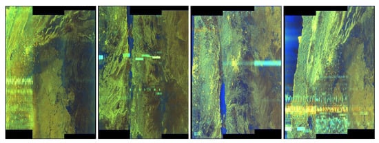
Figure 1.
Example of results that contain radio-frequency interference (RFI) artifacts.
Both manmade and natural sources can generate undesired signals that may cause RFI [16] capable of disrupting SAR images. These incoherent electromagnetic interference signals usually appear as various kinds of bright linear features [17,18] in the form of bright stripes with curvature or dense raindrops [2,4]. RFI can also contaminate image through slight haziness [2,18] that severely degrades the quality [4,17]. Unfortunately, such affected data may lead to incorrect interpretation processes and results [2].
Several methods for detection and reduction of RFI artifacts, particularly in SAR data, have been developed throughout the recent years (e.g., [19,20,21,22,23,24,25,26]; see also [2,27] for a general review). For SAR measurements, the most susceptible for RFI occurrence are signals operating in low band frequency regions, such as the P-, L-, S-, and even C-bands [2,17,18].
This paper on RFI artifact detection in C-band Sentinel-1 SAR data was initially motivated by the urgent need to develop a module—a part of the automatic monitoring system that is created for high-energy para-seismic events—that will support the automatic processing workflow through the exclusion of faulty SAR images (with artifacts) that might result in misinterpretation because RFI cases were noticeable in the area of interest. The deployed system uses the permanent scatterers in SAR (PSInSAR) method, which exploits long stacks of co-registered SAR images for analytical purposes to identify coherent points that provide consistent and stable response to the radar on board of a satellite [28]. Phase information obtained from these persistent scatterers is used to derive the ground displacement information and its temporal evolution [29].
Our ambition is to provide a robust and easy-to-implement method for marking images with RFI artifacts. Due to the constant and systematic availability of data, contaminated data can be eliminated, and thus, failure mitigation is not required in our system. RFI recognition remains the most crucial issue in this case.
For the purpose of RFI detection, we proposed a solution based on image processing methods with the use of feature extraction involving pixel convolution in our previous work [30], as well as thresholding and nearest neighbor structure filtering techniques and, as the reference classifier, we also used a convolutional neural network. Despite the positive results of this approach, to improve and develop our system, in this paper, we present deep learning techniques for the recognition of RFI artifacts at different levels of image damage appearing in Sentinel-1 SAR images and the use of complex convolutional neural networks.
In contrast to most RFI studies, which are usually conducted on raw data [2,4,17,18,31], our research is based on quick-look images included in Sentinel-1 data packages. Moreover, our efforts focused on the application of artificial intelligence techniques, such as deep learning methods, for RFI recognition, as foreseen by Tao [2] and Itschner [32]. This approach has proved very successful in recent works, e.g., [5,33,34,35], and it seems to be a proper direction for future investigations on effective methods for detection of these undesired failures.
The organization of this paper is arranged as follows. Section 2 introduces the definition of RFI, its characteristics, common forms, and sources. Then, the materials used and methodology applied based on deep learning are presented in Section 3 and Section 4, respectively. Section 5 depicts the experimental session, and Section 6 and Section 7 present the outcomes and interpretation of the results obtained. The final conclusions are presented in Section 8.
2. RFI Characteristics
Active remote sensing measurements with radar, including SAR, are continuously at risk of RFI, which is defined as “the effect of unwanted energy due to one or a combination of emissions, radiations, or inductions upon reception in a radio communication system, manifested by any performance degradation, misinterpretation, or loss of information which could be extracted in the absence of such unwanted energy” [36]. RFI may have a negative impact on the desired radar measurements, starting from the raw data, then the image formation process, and the interpretation of the final results [2].
The potential sources of RFI artifacts in SAR images are the many various radiation sources that operate within the same frequency band as the SAR system [2,17]. Two main groups of incoherent electromagnetic interference signal emitters can be distinguished—terrestrial and space-borne [2]. Most terrestrial RFI cases are connected with human activity over land, e.g., commercial or industrial radio devices [2], communication systems, television networks, air-traffic surveillance radars, meteorological radars, radiolocation radars, amateur radios, and other—mainly military-based—radiation sources [1,2,4,17,18]. The examples of space-borne RFI sources are signals broadcasting from other satellites, such as global navigation satellite system (GNSS) constellations, communication satellites, or other active remote sensing systems [2].
In recent years, many RFI cases have been observed in Sentinel-1 data products, with both terrestrial [31,37,38] and space-borne origin [1]. The major reason for these contaminations was probably military radars [18].
These incoherent electromagnetic interference signals usually affect the SAR signals operating in low frequency regions, such as the P-, L-, S-, and C-bands [2,17,18]. In this paper, we address RFI cases occurring at the C-band (frequency ranging from 4000–8000 MHz). This is one of the most important bands for radar science imaging [1], and particularly for Sentinel-1 satellites. These SAR radars operate in the 5350–5470 MHz band.
Over the last years, the European Space Agency (ESA) has reported an increase in RFI at the C-band in SAR data [1,39] that appears as short, strong bursts indicative of ground-based radar [1]. Although there are many different forms of RFI, generally, they can be grouped into four categories as follows [1,2,4]:
Narrow-band RFI—this kind of interference usually has a narrower bandwidth than that of the SAR system, and appears in the form of bright lines in images, which makes them easy to identify and detect [2,4]. Common sources (Figure 2) of this contamination are commercial land-mobile radios and amateur radios [1,2].
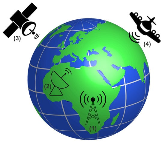
Figure 2.
Example of the common RFI sources: (1) radios, (2) radars, (3) communication systems, and (4) airborne sensors.
Pulsed RFI—this irregularity is pulsed in time, with or without pulse repetition, and may have bandwidths that are narrow or wide with respect to the sensor bandwidth [1]. In SAR images, it can be visible as bright marks or rectangles that are pulsed and sparse in time [40]. Typical sources (Figure 2) of this interference are ground-based radiolocation radars [1,2].
Broad-band (noise-like) RFI—in this case, signals have relatively broad bandwidth because of modulation, and are typically continuous in time regarding the radar integration time [1,2]. This type of interference has a noise-like characteristic; thus, it appears as image blurring or haziness along stripes. Common cases (Figure 2) of this RFI come from communication systems and other coded signals, such as GNSSs [1,2].
Heterogeneous RFI environments—these are multiple RFI emitters of different types that can be observed simultaneously, either within the main beam or the extended side lobes [1,2]. This RFI problem is particularly significant for airborne and space-borne sensors (Figure 2) that have a wide geographic field of view, such as an SAR system with a wide illuminated swath [1].
3. Materials
We participate in the project focusing on the development of the automatic monitoring system for high-energy para-seismic events and their influence on the surface with the use of GNSS, seismic, and PSInSAR techniques. Our project is based on Sentinel-1 data—in particular, Level-1 single-look complex (SLC) products—due to their numerous advantages. First of all, these data are available systematically and free of charge, without limitations, to all data users, including the general public and scientific and commercial users [41]. Moreover, they characterize a wide ground coverage and fine resolution because the Sentinel-1 SAR instrument mainly operates in the interferometric wide (IW) swath mode over land [14,41]. It is one of four Sentinel-1 acquisition modes that uses the terrain observation with progressive scans SAR (TOPSAR) technique [42] and provides data with a large swath width of 250 km at 5 m × 20 m (range × azimuth) spatial resolution for single-look data.
To evaluate the usefulness of the single Sentinel-1 data product, we exploit quick-look images contained in the preview folder, a part of the Sentinel-1 data package. These images are lower-resolution versions of the source images; thus, it is easy to quickly detect RFI artifacts and, as a consequence, eliminate contaminated data before further processing because they could lead to misinterpretation of the final results. This approach improves the whole PSInSAR processing workflow, which requires a stack of 25–30 SAR images in our case to calculate the ground displacements. Most importantly, exclusion of failure data does not affect the quality and reliability of the data processing results, as data are obtained continuously and observations can be repeated with a frequency better than six days, considering two satellites (Sentinel 1A and 1B) and both ascending and descending passes [41].
In order to develop a module that ensures effective detection and recognition of RFI artifacts, we chose a representative quick-look dataset named TELAVIV for the needs of our research. The reason is that, in order for the trained artificial neural network to be able to capture the necessary features unambiguously, the key point is that the training database should be large enough and should include various RFI cases as much as possible [2].
The characteristics of the interference depend strongly on the geographic position of data acquisition [2], and the ESA has reported an increase in the amount of RFI observed at the C-band [1]. Therefore, our selection is based on the map of RFI power in the C-band with continental coverage over Europe [31], the IEEE GRSS (IEEE Geoscience and Remote Sensing Society) RFI Observations Display System [43], and localization of RFI sources [44]. This collection consists of exactly 3602 images acquired from October 2014 (Sentinel-1A) and September 2016 (Sentinel-1B) until July 2020, and comprise the area surrounding the most populous city in the Gush Dan metropolitan area of Israel. The TELAVIV quick-look dataset is a subset of all obtained images, and contains 2591 elements. It was divided into four classes of almost equal size (if possible), with different levels of RFI contamination: 0 (clear/no artifacts), I (very weak/hardly visible artifacts), II (weak/few artifacts), and III (strong/many artifacts). This classification was conducted manually, and the number of rows with noticeable RFI artifacts and the intensity of contamination were taken into account.
Within this experimental dataset, we identified all types and forms of RFI (Figure 3), from narrow-band and its characteristic bright lines in images, through pulsed artifacts in the form of repeated pale rectangles, and ending with broad-band RFI and its blurring effect in images. We can easily state that here, we are facing a heterogeneous RFI environment that is a challenging test bed for our solution for RFI artifact detection.
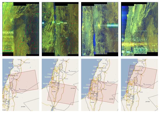
Figure 3.
Examples of different forms of RFI artifacts (and their localization) included in the training database.
The potential reason for the incoherent electromagnetic interference signals in the SAR images in the area surrounding Tel Aviv can be various radiation sources from the Sde Dov Airport, the Israel Defense Forces headquarters, and a large military base, as well as ships in the Mediterranean basin. In the case of broad-band RFI, many strong stripes with high intensity that produce irregular texture patterns and can be observed in many C-band Sentinel-1 SAR data acquired for this area are probably caused by simultaneous SAR imaging of the same area by both the Sentinel-1 and Canadian Radarsat-2 [1,45]. They both operate at the same center frequency of 5405 GHz [2,41].
In the next section, we introduce the motivation and basic information about the techniques we used in the experimental part.
4. Motivation and Methodology
Our main motivation was to verify the experimental effectiveness of recognizing artefacts with different levels of visibility on satellite images. As a reference classifier we have chosen the LeNet type convolutional neural network [46,47]—the general scheme is shown in Figure 4. The exact architecture of the network used can be seen in Section 4.1 and Figure 5.
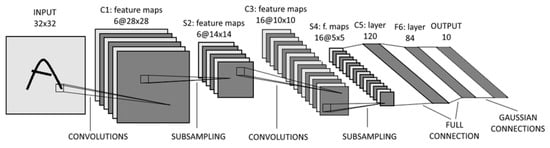
Figure 4.
Architecture of the convolutional neural network (LeNet)—image source [48].
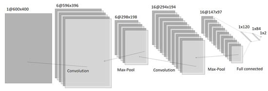
Figure 5.
Architecture of the convolutional neural network (LeNet)—a tool used to build the diagram: [49].
4.1. Deep Neural Network Architecture
To verify the effectiveness of our artifact extraction method, we used a LeNet deep neural network [46,48,50] defined in this section for classification. We used Python-related tools, such as PyTorch, TorchVision, and NumPy. The visualization of results was performed using Seaborn and Matplotlib. A transformation was made when loading images by scaling everything to 400 × 600 pixels to ensure the same size of the input for the network. The data were divided into training and testing sets in an 80/20 ratio in a random way. The network was fed with data after two alternating convolutional and maxpooling steps. We used three layers of neurons. The activation function of hidden layers was RELU; in the output layer we had raw values. The loss function took the form of categorical cross-entropy; thus, it can be higher than one. While the neural network learned, we used three data streams: R, G, and B. The Adam optimizer [51] was used. The training was done over 20 epochs. The batch size was 50 and the learning rate was 0.001. The layers used in our model can be seen in Figure 5.
Now allow us to explain in brief the use of various options of our model. Convolutional layers are used to extract features from images before they are fed into the network. We used max pooling because it is the most effective technique for reducing the sizes of images, which works well with neural network models. It turns out to be better in practice than average pooling [52].
5. Experimental Session
Let us now discuss what is new in relation to our previous research work [30].
Discussion of the Results Concerning Our Previous Studies
In this work, we are testing the effectiveness of learning by means of deep neural networks to recognize detailed levels of damage, and we do not go into the details of data pre-processing. In previous studies, we have looked for techniques to expose artifacts and checked their impact on the accuracy of recognition by observing the changing learning level of neural networks. We have observed that our methods have allowed the network to operate much more efficiently after pre-processing. We have discovered that the most effective technique of detecting artifacts from among the ones we have studied is the use of thresholding based on histograms of pixel values and noise filtering using the closest neighbors method. Pre-processing techniques were necessary because we used a small number of available learning objects. Examples of results for the RIYADH dataset from the previous work before and after the application of pre-processing are shown in Figure 6.
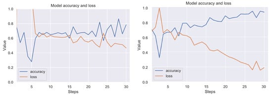
Figure 6.
Exemplary learning effect before (left side) and after using our technique (right side). Results for the RIYADH dataset. Class ok (without artifacts) vs. class er (with strong artifacts). The line graphs show accuracy (blue) and loss (orange) for 15 epochs (30 steps from batch). Although the image dataset is relatively small for the convolutional neural network (CNN), a good trend in increasing accuracy while minimizing loss can be observed.
The available number of objects in the TELAVIV dataset is suitable for deep learning, which allowed us to carry out relevant research on the possibilities of detecting artifacts on three separate levels of difficulty.
As a demo system, we chose the TELAVIV image set from open repository. We grouped the set into four classes—see Table 1. Samples of images representing classes can be seen in Figure 7.

Table 1.
The information about the decision classes.
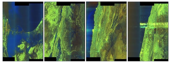
Figure 7.
TELAVIV quick-looks—exemplary pictures—first on the left without artifacts, and the subsequent images to the right, with increasing degrees of damage: classes 0, I, II, and III.
We treated this system as balanced, so we used global accuracy, which is defined as the percentage of correctly classified objects throughout the decision-making system.
In the experiments with deep neural network classification—see details in Section 4.1—the image sets were divided into a training subset where the network is taught and the validation test set, which comprised 20% of the objects on which the final neural network was tested. To estimate the quality of the classification, we used the Monte Carlo cross-validation [46,53] five technique (MCCV5, i.e., training and testing five times), presenting average results. In experiments, the test (validation) system was applied in a given iteration to the model to check the final efficiency and to observe the level of overfitting. In each iteration of learning of an independent validation set (not affecting the learning process of the network), by evaluating, we were able to determine the degree of generalization of the model. The result is objective at the moment when there is no process of overtraining, i.e., a clear discrepancy between the loss during network training and that resulting from testing the validation set.
We considered the following classification options from Table 2. We considered dropout options to check the level of overtraining reduction for better generalization of neural network learning. Looking at the results of the binary classification and the poor score for the class with the least visible damage, we decided to skip the network learning for all classes together. What we achieved was separate networks to detect each of the damage levels and a network showing whether or not there is a damaged image, without distinguishing the level of damage.
Table 2.
Considered classification options.
6. Results for the TELAVIV Dataset
In the experiment, we examined the separation of class 0 from classes III, II, and I, as well as from all at once. All experiments are performed in a similar pattern. Our results show how the MCCV-5 method works in each learning epoch. We present the results of five internal tests and the average result.
First of all, we show demonstrably very detailed results for variant class 0 vs. class 3. We present the accuracy of classification and entropy loss of a given variant—see, e.g., Figure 8. Then, we present what the classification of the validation test systems looked like in a given iteration and subtest—see, e.g., Figure 9. We then show the combined average results by adding the standard deviation in the form of vertical lines in individual epochs—see, e.g., Figure 10 and Figure 11. The standard deviation was calculated from individual subtests of the MCCV method.
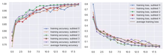
Figure 8.
Class 0 vs. Class III. Model: the LeNet model from Figure 5 was applied. Validation technique: cross-validation 5. Accuracy for 20 iterations of neural network training and corresponding cross-entropy loss.
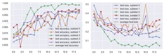
Figure 9.
Class 0 vs. Class III. Model: the LeNet model from Figure 5 was applied. Validation technique: cross-validation 5. Accuracy for 20 iterations of neural network training and corresponding cross-entropy loss. Validation takes place after every epoch of learning.
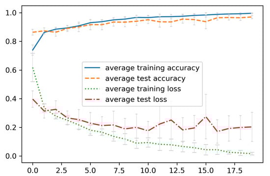
Figure 10.
Summary of average results for 20 iterations. Class 0 vs. III. Model: the LeNet model from Figure 5 was applied. Validation method: cross-validation 5. Accuracy for 20 iterations of neural network training.
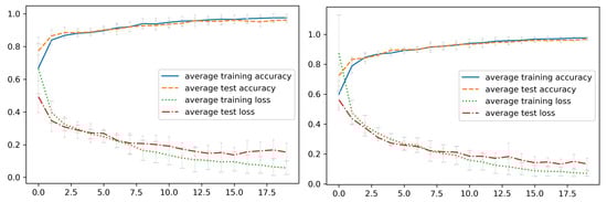
Figure 11.
Left image: single dropout. Right image: double dropout. Summary of average results for 20 iterations. Class 0 vs. III. Model: the LeNet model from Figure 5 was applied. Cross-validation 5. Accuracy for 20 iterations of neural network training and corresponding cross-entropy loss.
Then, we show the analogous result for the other pairs of classes, taking into account only average results with standard deviation. In Figure 12 and Figure 13, we have the results for the class 0 vs. class 2 variant. In Figure 14 and Figure 15, we have the results for the class 0 vs. class 1 variant. Finally, in Figure 16 and Figure 17, we have the result for the class 0 vs. all variant.
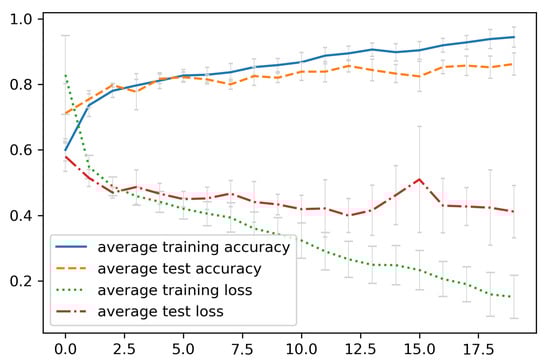
Figure 12.
Summary of average results for 20 iterations. Class 0 vs. II. Model: the LeNet model from Figure 5 was applied. Cross-validation 5. Accuracy for 20 iterations of neural network training and corresponding cross-entropy loss.
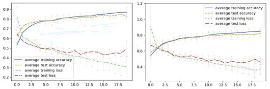
Figure 13.
Left image: single dropout. Right image: double dropout. Summary of average results for 20 iterations. Class 0 vs. II. Single dropout. Model: the LeNet model from Figure 5 was applied. Cross-validation 5. Accuracy for 20 iterations of neural network training and corresponding cross-entropy loss.
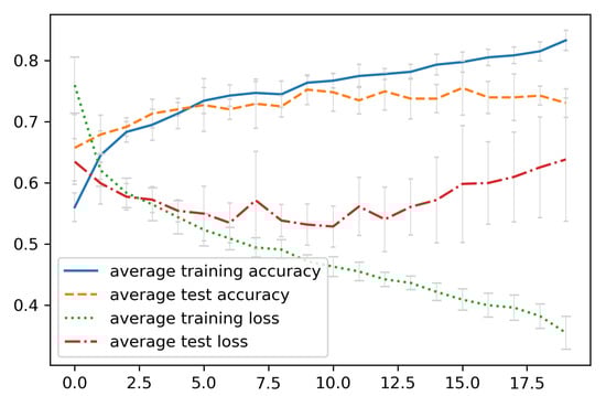
Figure 14.
Summary of average results for 20 iterations. Class 0 vs. I. Model: the LeNet model from Figure 5 was applied. Cross-validation 5. Accuracy for 20 iterations of neural network training and corresponding cross-entropy loss.
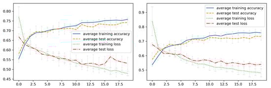
Figure 15.
Left image: single dropout. Right image: double dropout. Summary of average results for 20 iterations. Class 0 vs. I. Single dropout. Model: the LeNet model from Figure 5 was applied. Cross-validation 5. Accuracy for 20 iterations of neural network training and corresponding cross-entropy loss.
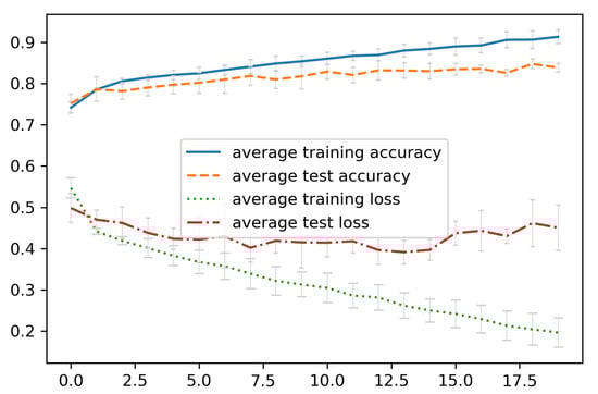
Figure 16.
Summary of average results for 20 iterations. Class 0 vs. All. Model: the LeNet model from Figure 5 was applied. Cross-validation 5. Accuracy for 20 iterations of neural network training and corresponding cross-entropy loss.
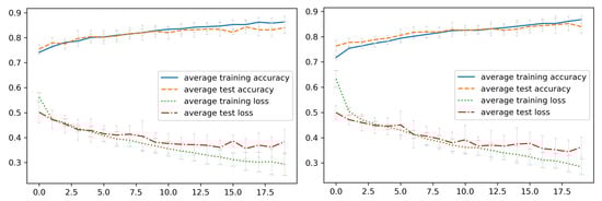
Figure 17.
Left image: single dropout. Right image: double dropout. Summary of average results for 20 iterations. Class 0 vs. All. Model: the LeNet model from Figure 5 was applied. Cross-validation 5. Accuracy for 20 iterations of neural network training and corresponding cross-entropy loss.
In the following sections, we present in the model discussed the results for all classification options with all planned variations of the neural network.
7. Discussion of Results
We got the average accuracy of 0.731 with a standard deviation of 0.023 in the 0 vs. I variant with the non-dropout variation. After using the single and double dropout, the learning process is stabilized with approximate average accuracies of 0.742 and 0.733, respectively, with a standard deviation of 0.013 and 0.026.
In the 0 vs. II variant with the non-dropout variation, we got the accuracy of 0.862 with a standard deviation of 0.034. After using the single and double dropout, the learning process is stabilized with approximate average accuracies of 0.829 and 0.823, respectively, with a standard deviation of 0.02 and 0.052 .
In the 0 vs. III variant with the non-dropout variant, we got the accuracy of 0.971 with a standard deviation of 0.01. After using the single and double dropout, the learning process clearly stabilized with approximate average accuracies of 0.962 and 0.968, respectively, with a standard deviation of 0.017 and 0.009.
In the 0 vs. All variant with the non-dropout variant, we got the accuracy of 0.838 with a standard deviation of 0.01. After using the single and double dropout, the learning process stabilized with approximate average accuracies of 0.84 and 0.84, respectively, with a standard deviation of 0.013 and 0.026.
In most cases, the dropout increases the standard deviation of validation results while eliminating overlearning. Despite being overlearned in the non-dropout variant, the validation result is similar to the dropout option.
Let us conclude our work.
8. Conclusions
In recent years, RFI cases have occurred more frequently in SAR measurements. Its characteristics, including various forms and sources, depend strongly on the geographical region of data acquisition. RFI ariefacts may have an adverse influence not only on the desired radar measurements, but also on the image formation or subsequent interpretation process. Therefore, it is important to search for the most appropriate solutions in this area that have the greatest impact on minimizing the negative effect of RFI disturbances in SAR data.
In this work, we proposed a data mining model for the detection of artifacts at different levels of image damage. We designed a convolutional neural network with automatic calculation of the image shape after pre-processing by means of convolutions and poolings. As a reference system, we used a collection of images from the TELAVIV collection. We verified in the learning process that dropout has no major impact on the quality of the final model for these particular data. The experimental results are very promising; as one could expect, the highest efficiency of 97% was obtained in the detection of strong artifacts. Detection of weak artifacts reaches 86% effectiveness. Detection of very weak artifacts reaches 74% accuracy. Eventually, detection of artifacts of all classes at once gives 84% effectiveness. The proposed solution can effectively support the automatic PSInSAR processing workflow by recognizing RFI-affected data and, as a consequence, removing them from the stack of SAR images required to determine the ground displacements. In conclusion, it is difficult to find a method for generalizing the problem of searching for artifacts. Each dataset containing artifacts should be treated individually. The model structure should be selected in a personalized way.
This work calls for several perspectives. We can take the results of the work as a reference for testing other neural network architects. An interesting thread may be to check the possibility of grouping images in different damage levels in an unsupervised manner.
Author Contributions
Conceptualization, P.A., J.R., and A.C.; methodology, software, validation, formal analysis, and investigation, P.A.; data acquisition and classification A.C.; resources, A.C. and P.A.; writing—original draft preparation, A.C. and P.A.; writing—review and editing, A.C. and P.A.; funding acquisition, J.R. All authors have read and agreed to the published version of the manuscript.
Funding
This research conducted under the project entitled “Automatic system for monitoring the influence of high-energy paraseismic tremors on the surface using GNSS/PSInSAR satellite observations and seismic measurements” (Project No. POIR.04.01.04-00-0056/17), co-financed by the European Regional Development Fund within the Smart Growth Operational Programm 2014–2020.
Conflicts of Interest
The authors declare no conflict of interest.
References
- National Academies of Sciences, Engineering, and Medicine. A Strategy for Active Remote Sensing Amid Increased Demand for Radio Spectrum; The National Academies Press: Washington, DC, USA, 2015. [Google Scholar] [CrossRef]
- Tao, M.; Su, J.; Huang, Y.; Wang, L. Mitigation of Radio Frequency Interference in Synthetic Aperture Radar Data: Current Status and Future Trends. Remote Sens. 2019, 11, 2438. [Google Scholar] [CrossRef]
- Ding, X.-L.; Li, Z.-W.; Zhu, J.-J.; Feng, G.-C.; Long, J.-P. Atmospheric Effects on InSAR Measurements and Their Mitigation. Sensors 2008, 8, 5426–5448. [Google Scholar] [CrossRef] [PubMed]
- Yang, L.; Zheng, H.; Feng, J.; Li, N.; Chen, J. Detection and suppression of narrow band RFI for synthetic aperture radar imaging. Chin. J. Aeronaut. 2015, 28, 1189–1198. [Google Scholar] [CrossRef]
- Yu, J.; Li, J.; Sun, B.; Chen, J.; Li, C. Multiclass Radio Frequency Interference Detection and Suppression for SAR Based on the Single Shot MultiBox Detector. Sensors 2018, 18, 4034. [Google Scholar] [CrossRef]
- Wang, J.; Yu, W.; Deng, Y.; Wang, R.; Wang, Y.; Zhang, H.; Zheng, M. Demonstration of Time-Series InSAR Processing in Beijing Using a Small Stack of Gaofen-3 Differential Interferograms. J. Sens. 2019. [Google Scholar] [CrossRef]
- Zebker, H.A.; Rosen, P.A.; Hensley, S. Atmospheric effects in interferometric synthetic aperture radar surface deformation and topographic maps. J. Geophys. Res. 1997, 102, 7547–7563. [Google Scholar] [CrossRef]
- Emardson, T.R.; Simons, M.; Webb, F.H. Neutral atmospheric delay in interferometric synthetic aperture radar applications: Statistical description and mitigation. J. Geophys. Res. 2003, 108, 2231–2238. [Google Scholar] [CrossRef]
- Liao, M.; Jiang, H.; Wang, Y.; Wang, T.; Zhang, L. Improved topographic mapping through high-resolution SAR interferometry with atmospheric removal. ISPRS J. Photogram. Remote Sens. 2013, 80, 72–79. [Google Scholar] [CrossRef]
- Hu, Z.; Mallorquí, J.J. An Accurate Method to Correct Atmospheric Phase Delay for InSAR with the ERA5 Global Atmospheric Model. Remote Sens. 2019, 11, 1969. [Google Scholar] [CrossRef]
- Liu, Z.; Zhou, C.; Fu, H.; Zhu, J.; Zuo, T. A Framework for Correcting Ionospheric Artifacts and Atmospheric Effects to Generate High Accuracy InSAR DEM. Remote Sens. 2020, 12, 318. [Google Scholar] [CrossRef]
- Stasolla, M.; Neyt, X. An Operational Tool for the Automatic Detection and Removal of Border Noise in Sentinel-1 GRD Products. Sensors 2018, 18, 3454. [Google Scholar] [CrossRef] [PubMed]
- Hajduch, G.; Miranda, N. Masking “No-Value” Pixels on GRD Products Generated by the Sentinel-1 ESA IPF; Document Reference MPC-0243; S-1 Mission Performance Centre, ESA: Paris, France, 2018. [Google Scholar]
- Ali, I.; Cao, S.; Naeimi, V.; Paulik, C.; Wagner, W. Methods to Remove the Border Noise From Sentinel-1 Synthetic Aperture Radar Data: Implications and Importance For Time-Series Analysis. IEEE J. Sel. Top. Appl. Earth Obs. Remote Sens. 2018, 11, 777–786. [Google Scholar] [CrossRef]
- Luo, Y.; Flett, D. Sentinel-1 Data Border Noise Removal and Seamless Synthetic Aperture Radar Mosaic Generation. In Proceedings of the 2nd International Electronic Conference on Remote Sensing, Online, 22 March–5 April 2018. [Google Scholar] [CrossRef]
- CISA. Radio Frequency Interference Best Practices Guidebook. Cybersecurity and Infrastructure Security Agency, SAFECOM/- National Council of Statewide Interoperability Coordinator. 2020. Available online: https://www.cisa.gov/sites/default/files/publications/safecom-ncswic_rf_interference_best_practices_guidebook_2.7.20_-_final_508c.pdf (accessed on 23 July 2020).
- Meyer, F.J.; Nicoll, J.B.; Doulgeris, A.P. Correction and Characterization of Radio Frequency Interference Signatures in L-Band Synthetic Aperture Radar Data. IEEE Trans. Geosci. Remote Sens. 2013, 51, 4961–4972. [Google Scholar] [CrossRef]
- Parasher, P.; Aggarwal, K.M.; Ramanujam, V.M. RFI detection and mitigation in SAR data. In Proceedings of the Conference: 2019 URSI Asia-Pacific Radio Science Conference (AP-RASC), New Delhi, India, 9–15 March 2019. [Google Scholar] [CrossRef]
- Forte, G.F.; Tarongí Bauza, J.M.; DePau, V.; Vall·llossera, M.; Camps, A. Experimental Study on the Performance of RFI Detection Algorithms in Microwave Radiometry: Toward an Optimum Combined Test. IEEE Trans. Geosci. Remote Sens. 2013, 51, 10. [Google Scholar] [CrossRef]
- Tierney, C.; Mulgrew, B. Adaptive waveform design with least-squares system identification for interference mitigation in SAR. In Proceedings of the IEEE Radar Conference, Seattle, WA, USA, 8–12 May 2017. [Google Scholar] [CrossRef]
- Cucho-Padin, G.; Wang, Y.; Li, E.; Waldrop, L.; Tian, Z.; Kamalabadi, F.; Perillat, P. Radio Frequency Interference Detection and Mitigation Using Compressive Statistical Sensing. Radio Sci. 2019, 54, 11. [Google Scholar] [CrossRef]
- Querol, J.; Perez, A.; Camps, A. A Review of RFI Mitigation Techniques in Microwave Radiometry. Remote Sens. 2019, 11, 3042. [Google Scholar] [CrossRef]
- Shen, W.; Qin, Z.; Lin, Z. A New Restoration Method for Radio Frequency Interference Effects on AMSR-2 over North America. Remote Sens. 2019, 11, 2917. [Google Scholar] [CrossRef]
- Soldo, Y.; Le Vine, D.; De Matthaeis, P. Detection of Residual “Hot Spots” in RFI-Filtered SMAP Data. Remote Sens. 2019, 11, 2935. [Google Scholar] [CrossRef]
- Johnson, J.T.; Ball, C.; Chen, C.; McKelvey, C.; Smith, G.E.; Andrews, M.; O’Brien, A.; Garry, J.L.; Misra, S.; Bendig, R.; et al. Real-Time Detection and Filtering of Radio Frequency Interference Onboard a Spaceborne Microwave Radiometer: The CubeRRT Mission. IEEE J. Sel. Top. Appl. Earth Obs. Remote Sens. 2020, 13. [Google Scholar] [CrossRef]
- Yang, Z.; Yu, C.; Xiao, J.; Zhang, B. Deep residual detection of radio frequency interference for FAST. Mon. Not. R. Astron. Soc. 2020, 492, 1. [Google Scholar] [CrossRef]
- Tarongí Bauza, J.M. Radio Frequency Interference in Microwave Radiometry: Statistical Analysis and Study of Techniques for Detection and Mitigation. Ph.D. Thesis, Department of Signal Theory and Communications, Universitat Politecnica de Catalunya, BarcelonaTech, Spain, 2012. Available online: https://www.tdx.cat/bitstream/handle/10803/117023/TJTB1de1.pdf (accessed on 23 July 2020).
- Ferretti, A.; Prati, C.; Rocca, F. Permanent Scatterers in SAR Interferometry. IEEE Trans. Geosci. Remote Sens. 2001, 39, 8–20. [Google Scholar] [CrossRef]
- Solari, L.; Ciampalini, A.; Raspini, F.; Bianchini, S.; Moretti, S. PSInSAR Analysis in the Pisa Urban Area (Italy): A Case Study of Subsidence Related to Stratigraphical Factors and Urbanization. Remote Sens. 2016, 8, 120. [Google Scholar] [CrossRef]
- Chojka, A.; Artiemjew, P.; Rapiński, J. RFI Artefacts Detection in Sentinel-1 Level-1 SLC Data Based On Image Processing Techniques. Sensors 2020, 20, 2919. [Google Scholar] [CrossRef] [PubMed]
- Monti-Guarnieri, A.; Giudici, D.; Recchia, A. Identification of C-Band Radio Frequency Interferences from Sentinel-1 Data. Remote Sens. 2017, 9, 1183. [Google Scholar] [CrossRef]
- Itschner, I.; Li, X. Radio Frequency Interference (RFI) Detection in Instrumentation Radar Systems: A Deep Learning Approach. In Proceedings of the IEEE Radar Conference (RadarConf) 2019, Boston, MA, USA, 22–26 April 2019. [Google Scholar] [CrossRef]
- Akeret, J.; Chang, C.; Lucchi, A.; Refregier, A. Radio frequency interference mitigation using deep convolutional neural networks. Astron. Comput. 2017, 18, 35–39. [Google Scholar] [CrossRef]
- Zhang, L.; You, W.; Wu, Q.M.J.; Qi, S.; Ji, Y. Deep Learning-Based Automatic Clutter/Interference Detection for HFSWR. Remote Sens. 2018, 10, 1517. [Google Scholar] [CrossRef]
- Fan, W.; Zhou, F.; Tao, M.; Bai, X.; Rong, P.; Yang, S.; Tian, T. Interference Mitigation for Synthetic Aperture Radar Based on Deep Residual Network. Remote. Sens. 2019, 11, 1654. [Google Scholar] [CrossRef]
- International Telecommunication Union. Radio Regulations Articles, Section VII—Frequency Sharing, Article 1.166, Definition: Interference, 2016. Available online: http://search.itu.int/history/HistoryDigitalCollectionDocLibrary/1.43.48.en.101.pdf (accessed on 23 July 2020).
- Recchia, A.; Giudici, D.; Piantanida, R.; Franceschi, N.; Monti-Guarnieri, A.; Miranda, N. On the Effective Usage of Sentinel-1 Noise Pulses for Denoising and RFI Identification. In Proceedings of the 12th European Conference on Synthetic Aperture Radar, Aachen, Germany, 4–7 June 2018; ISBN 978-3-8007-4636-1. [Google Scholar]
- Leng, X.; Ji, K.; Zhou, S.; Xing, X.; Zou, H. Discriminating Ship from Radio Frequency Interference Based on Noncircularity and Non-Gaussianity in Sentinel-1 SAR Imagery. IEEE Trans. Geosci. Remote Sens. 2019, 57, 1. [Google Scholar] [CrossRef]
- Franceschi, N.; Piantanida, R.; Recchia, A.; Giudici, D.; Monti-Guarnieri, A.; Miranda, N.; Albinet, C. RFI Monitoring and Classification in C-band Using Sentinel-1 Noise Pulses. In Proceedings of the RFI 2019 Workshop: Coexisting with Radio Frequency Interference, Toulouse, France, 23–27 September 2019; Available online: http://www.ursi.org/proceedings/2019/rfi2019/23p4.pdf (accessed on 23 July 2020).
- Spencer, M.; Ulaby, F. Spectrum Issues Faced by Active Remote Sensing: Radio frequency interference and operational restrictions Technical Committees. IEEE Geosci. Remote. Sens. Mag. 2016, 4, 1. [Google Scholar] [CrossRef]
- ESA. Sentinel Online Technical Website. Sentinel-1. 2020. Available online: https://sentinel.esa.int/web/sentinel/missions/sentinel-1 (accessed on 23 July 2020).
- De Zan, F.; Monti-Guarnieri, A. TOPSAR: Terrain Observation by Progressive Scans. IEEE Trans. Geosci. Remote Sens. 2006, 44, 2352–2360. [Google Scholar] [CrossRef]
- IEEE FARS Technical Committee. Database of Frequency Allocations for Microwave Remote Sensing and Observed Radio Frequency Interference. 2020. Available online: http://grss-ieee.org/microwave-interferers/ (accessed on 23 July 2020).
- Soldo, Y.; Cabot, F.; Khazaal, A.; Miernecki, M.; Slominska, E.; Fieuzal, R.; Kerr, Y.H. Localization of RFI sources for the SMOS mission: A means for assessing SMOS pointing performances. IEEE J. Sel. Top. Appl. Earth Obs. Remote Sens. 2015, 8, 617–627. [Google Scholar] [CrossRef]
- Meadows, P.J.; Hajduch, G.; Miranda, N. Sentinel-1 Long Duration Mutual Interference; Document Reference MPC-0432; S-1 Mission Performance Centre, ESA: Paris, France, 2018; Available online: https://sentinel.esa.int/documents/247904/2142675/Sentinel-1-Long-Duration-Mutual-Interference (accessed on 23 July 2020).
- Goodfellow, I.; Bengio, Y.; Courville, A. Deep Learning; The MIT Press: London, UK, 2016; ISBN 978-0262035613. [Google Scholar]
- Lou, G.; Shi, H. Face image recognition based on convolutional neural network. China Commun. 2020, 17, 2. [Google Scholar] [CrossRef]
- Lecun, Y.; Bottou, L.; Bengio, Y.; Haffner, P. “Gradient-based learning applied to document recognition” (PDF). Proc. IEEE 1998, 86, 2278–2324. [Google Scholar] [CrossRef]
- LeNail, A. NN-SVG: Publication-Ready Neural Network Architecture Schematics. J. Open Source Softw. 2019, 4, 747. Available online: http://alexlenail.me/NN-SVG/LeNet.html (accessed on 27 November 2020). [CrossRef]
- Almakky, I.; Palade, V.; Ruiz-Garcia, A. Deep Convolutional Neural Networks for Text Localisation in Figures from Biomedical Literature. In Proceedings of the International Joint Conference on Neural Networks (IJCNN) 2019, Budapest, Hungary, 14–19 July 2019. [Google Scholar] [CrossRef]
- Kingma, D.P.; Ba, J. Adam: A method for stochastic optimization. In Proceedings of the 3rd International Conference for Learning Representations, San Diego, CA, USA, 7–9 May 2015. [Google Scholar]
- Brownlee, J. A Gentle Introduction to Deep Learning for Face Recognition, May 31, 2019 in Deep Learning for Computer Vision. Available online: https://machinelearningmastery.com/introduction-to-deep-learning-for-face-recognition/ (accessed on 23 July 2020).
- Xu, Q.-S.; Liang, Y.-Z. Monte Carlo cross validation. Chemom. Intell. Lab. Syst. 2001, 56, 1. [Google Scholar] [CrossRef]
Publisher’s Note: MDPI stays neutral with regard to jurisdictional claims in published maps and institutional affiliations. |
© 2020 by the authors. Licensee MDPI, Basel, Switzerland. This article is an open access article distributed under the terms and conditions of the Creative Commons Attribution (CC BY) license (http://creativecommons.org/licenses/by/4.0/).