Landslide Mapping and Monitoring Using Persistent Scatterer Interferometry (PSI) Technique in the French Alps

 , ,
, ,
Abstract
1. Introduction
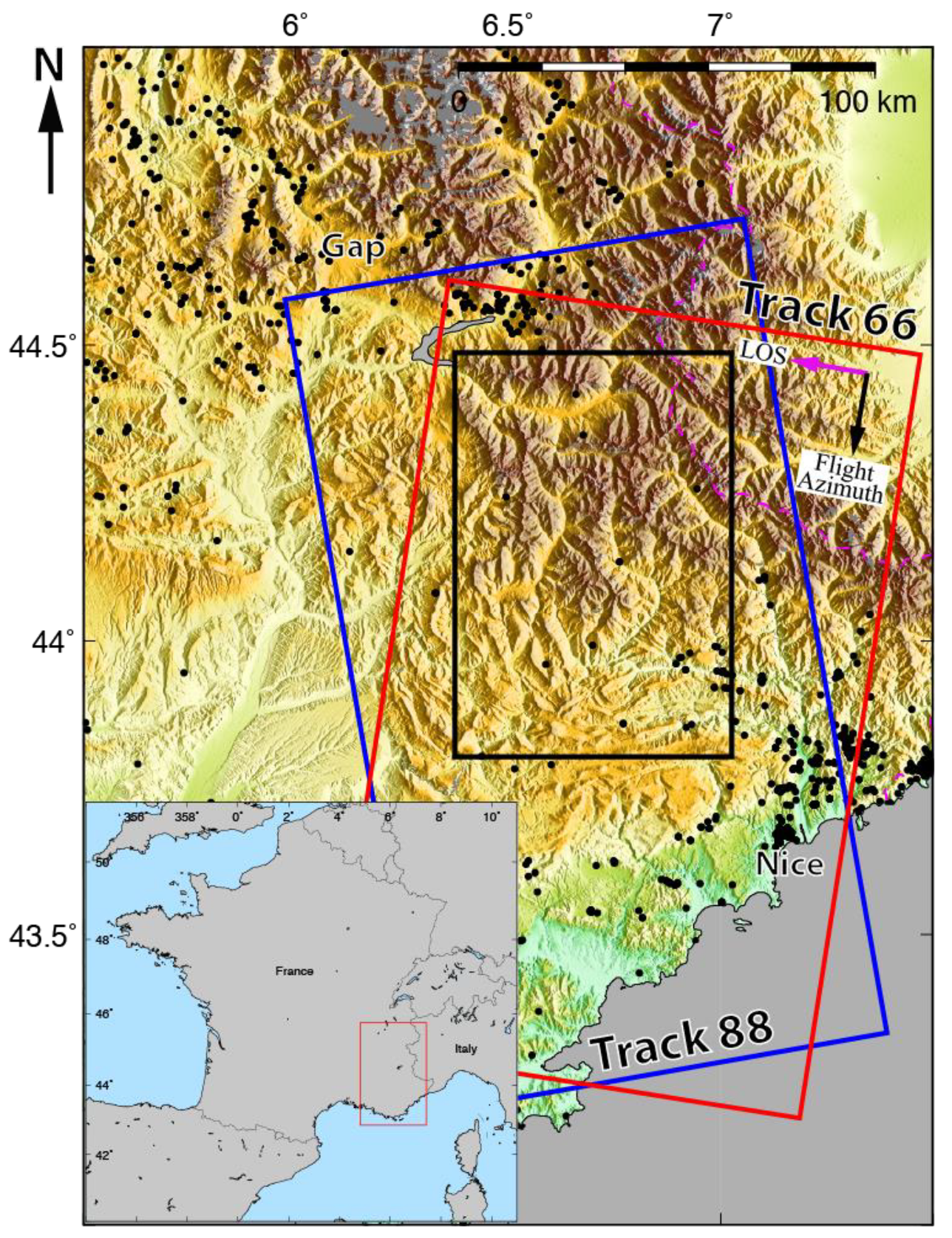
2. Study Area
Previous Measurements of Slope Movements in the French Alps
3. Datasets and Methodology
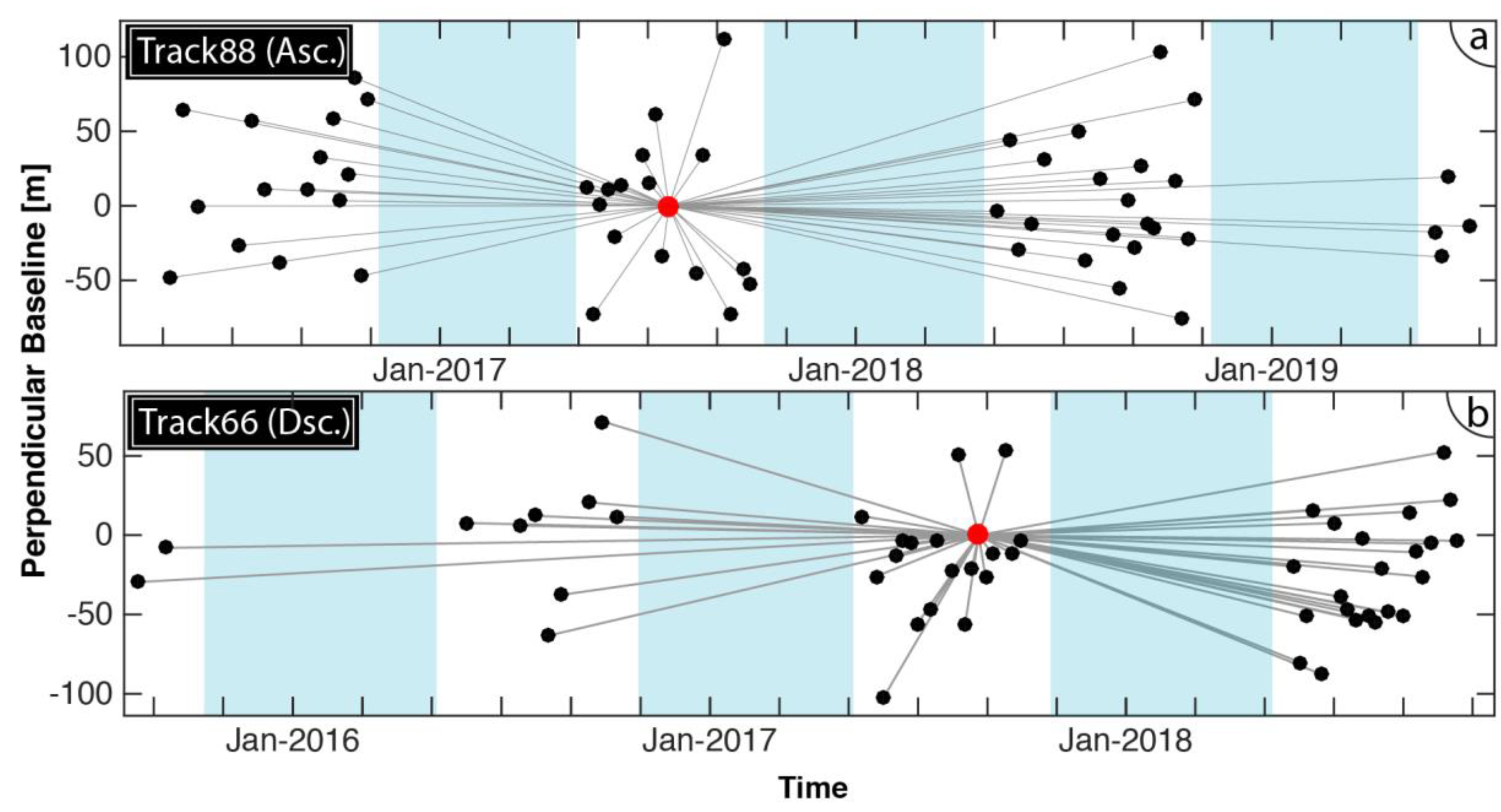
3.1. InSAR Datasets
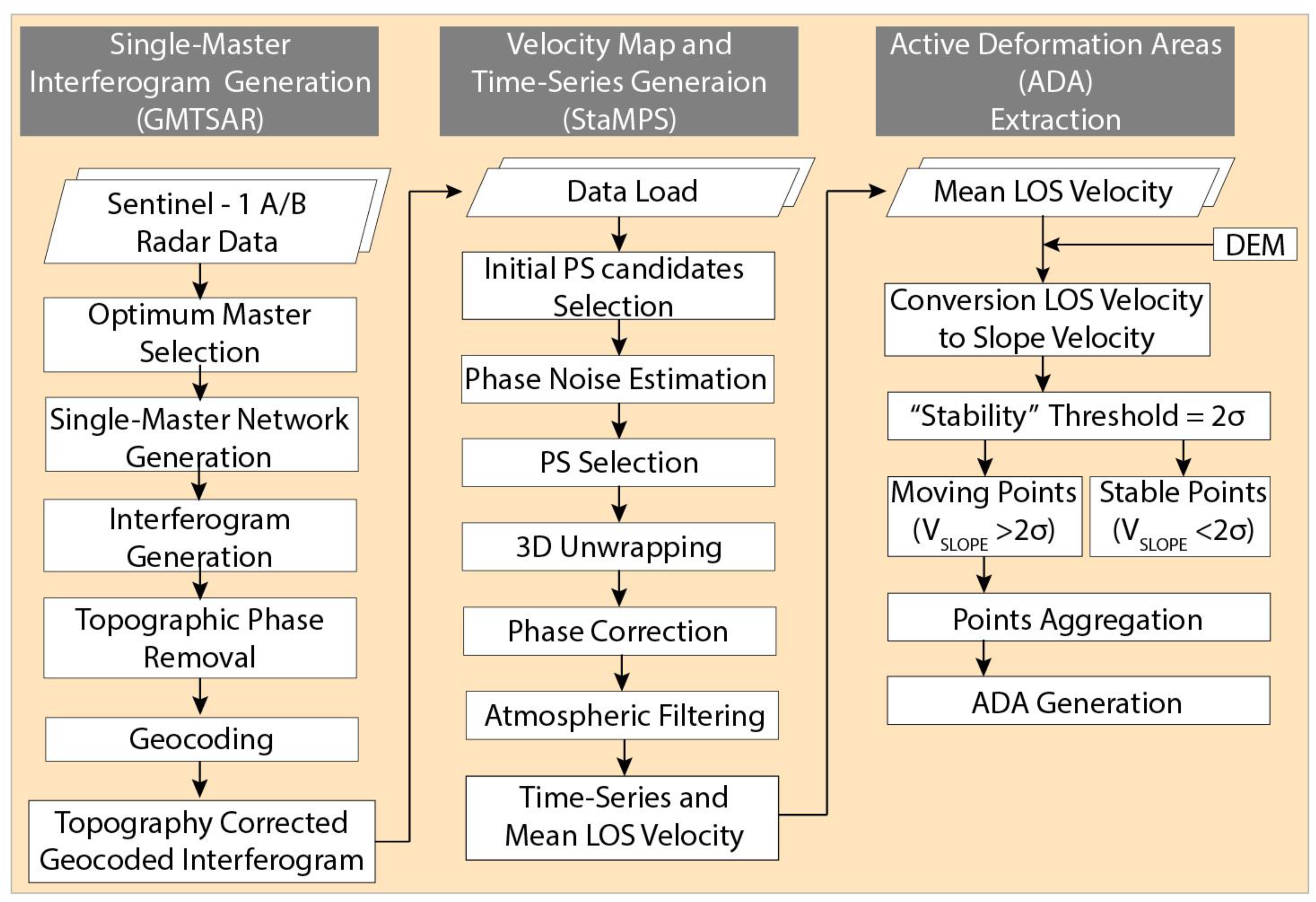
3.2. Methodology of Landslide Mapping
3.3. PSI Processing Methodology
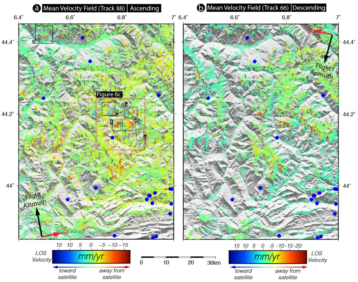
3.4. InSAR-Derived Mean Velocity Maps
3.5. Limitation of PSI Technique in Landslide Detection
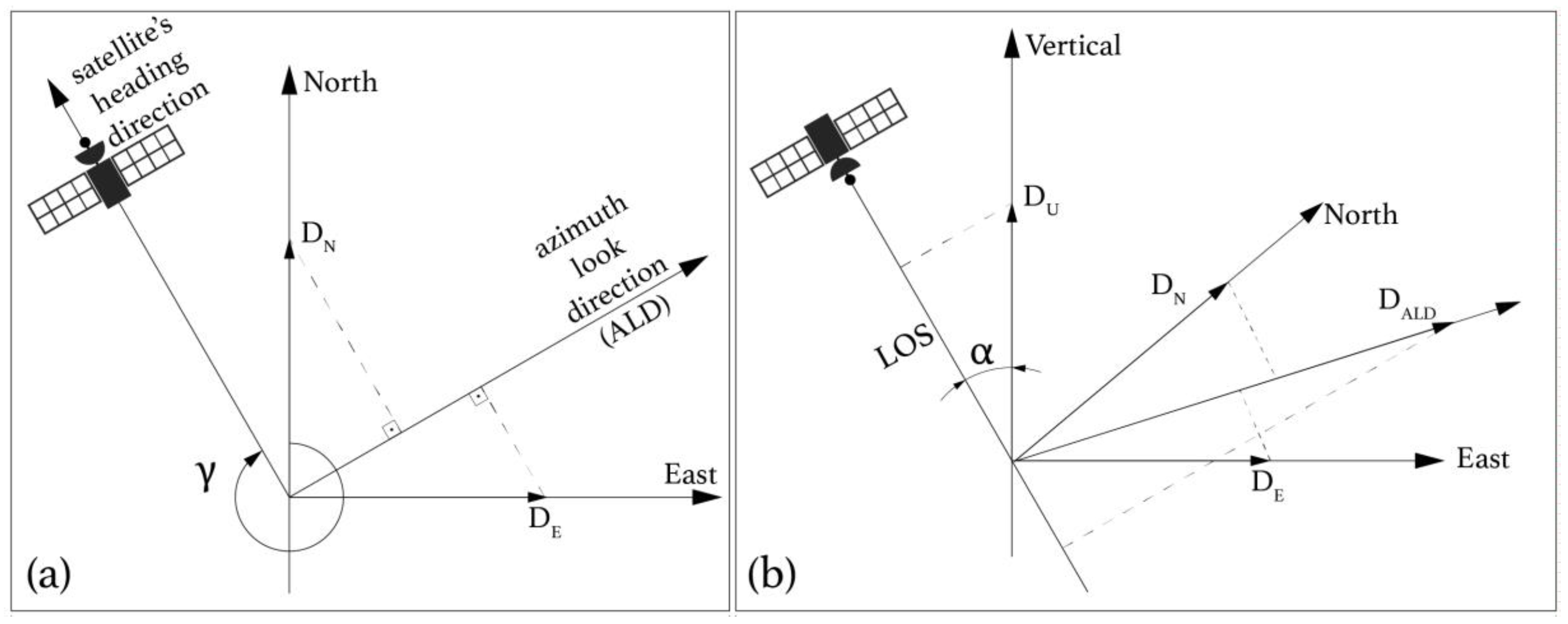
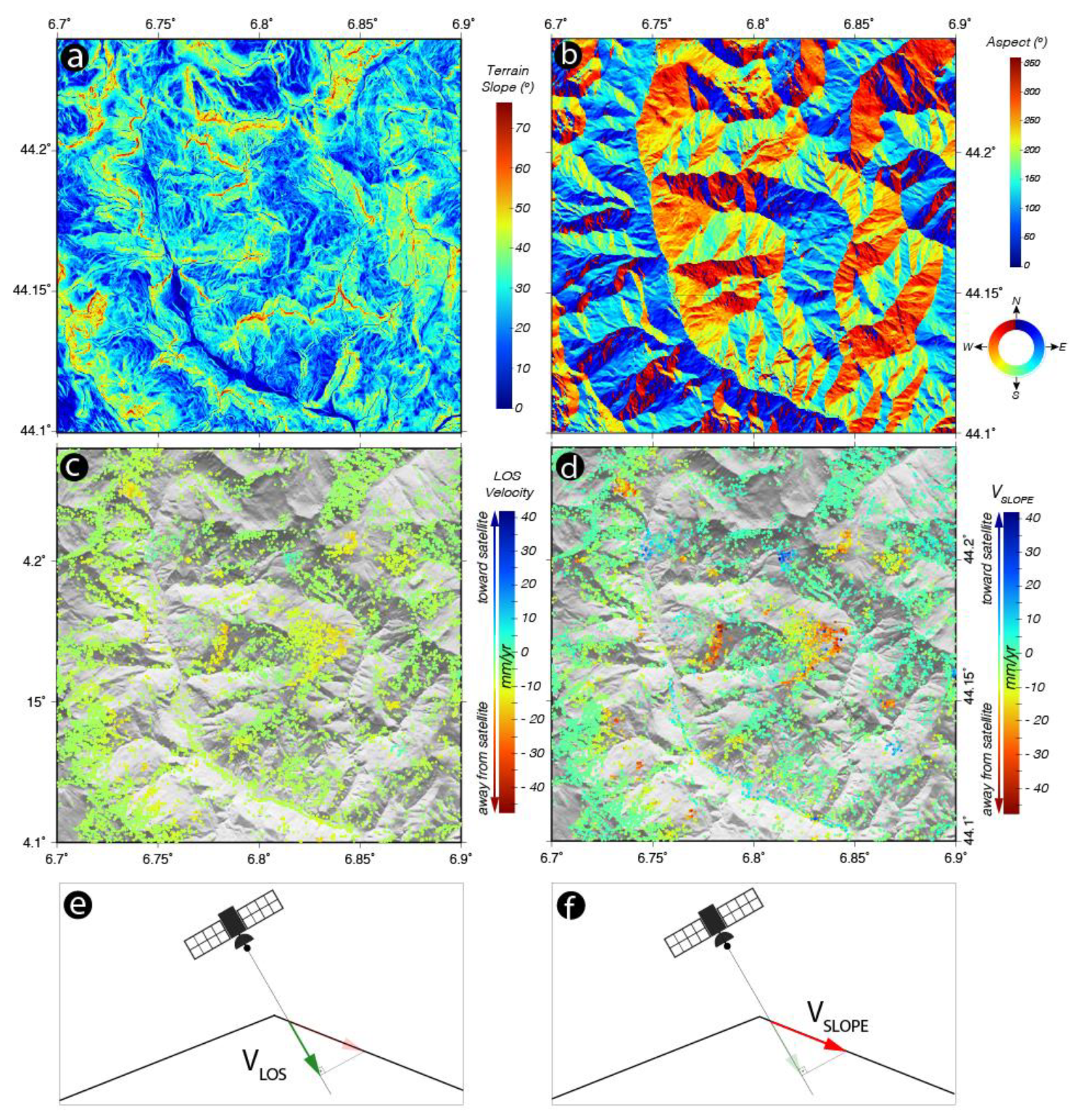
3.6. Projection from VLOS to VSLOPE
3.7. Detection of Active Deformation Areas (ADA)
4. Discussion
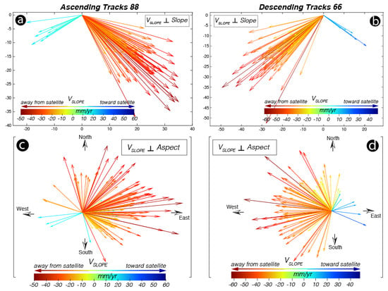
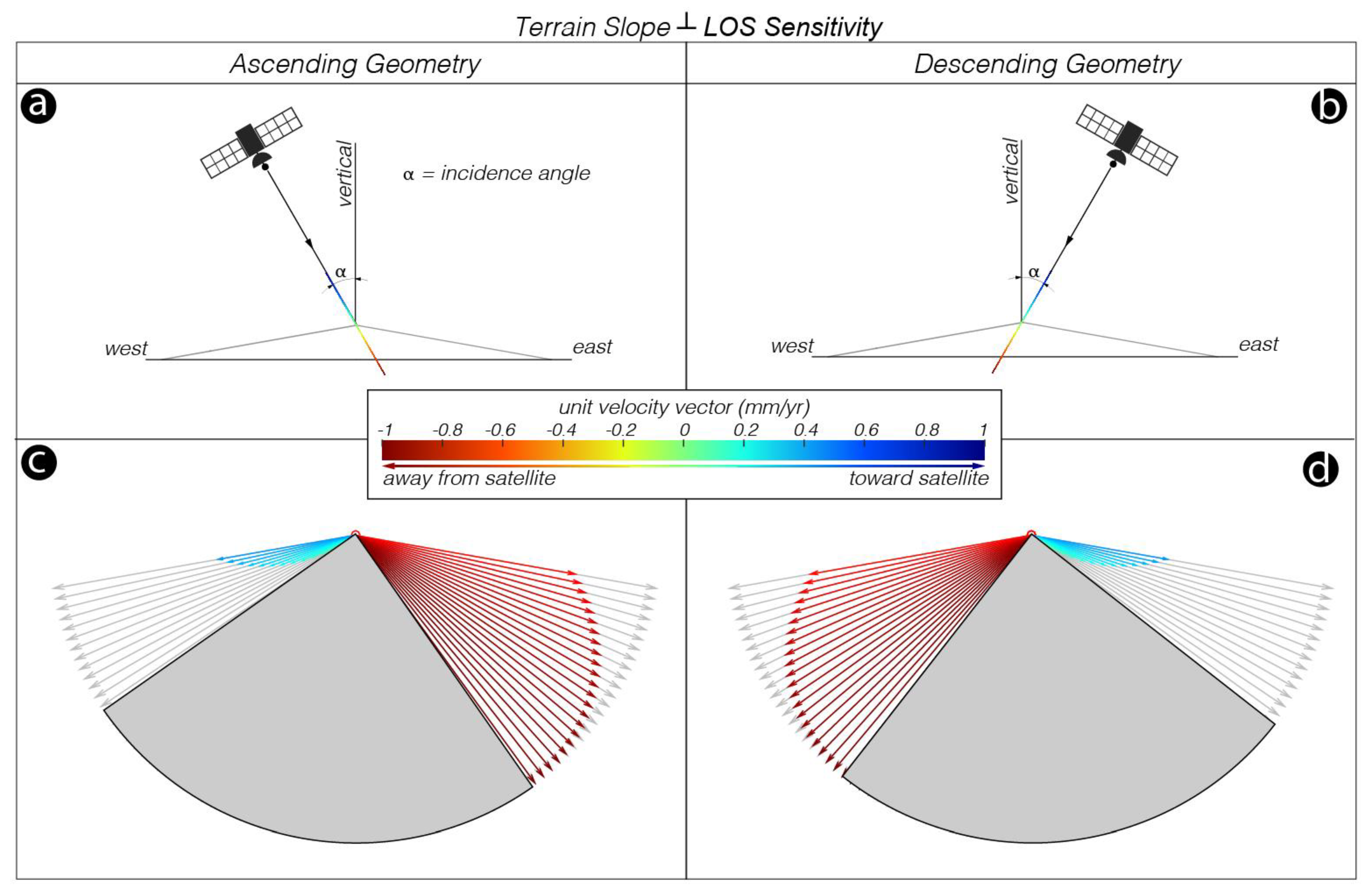
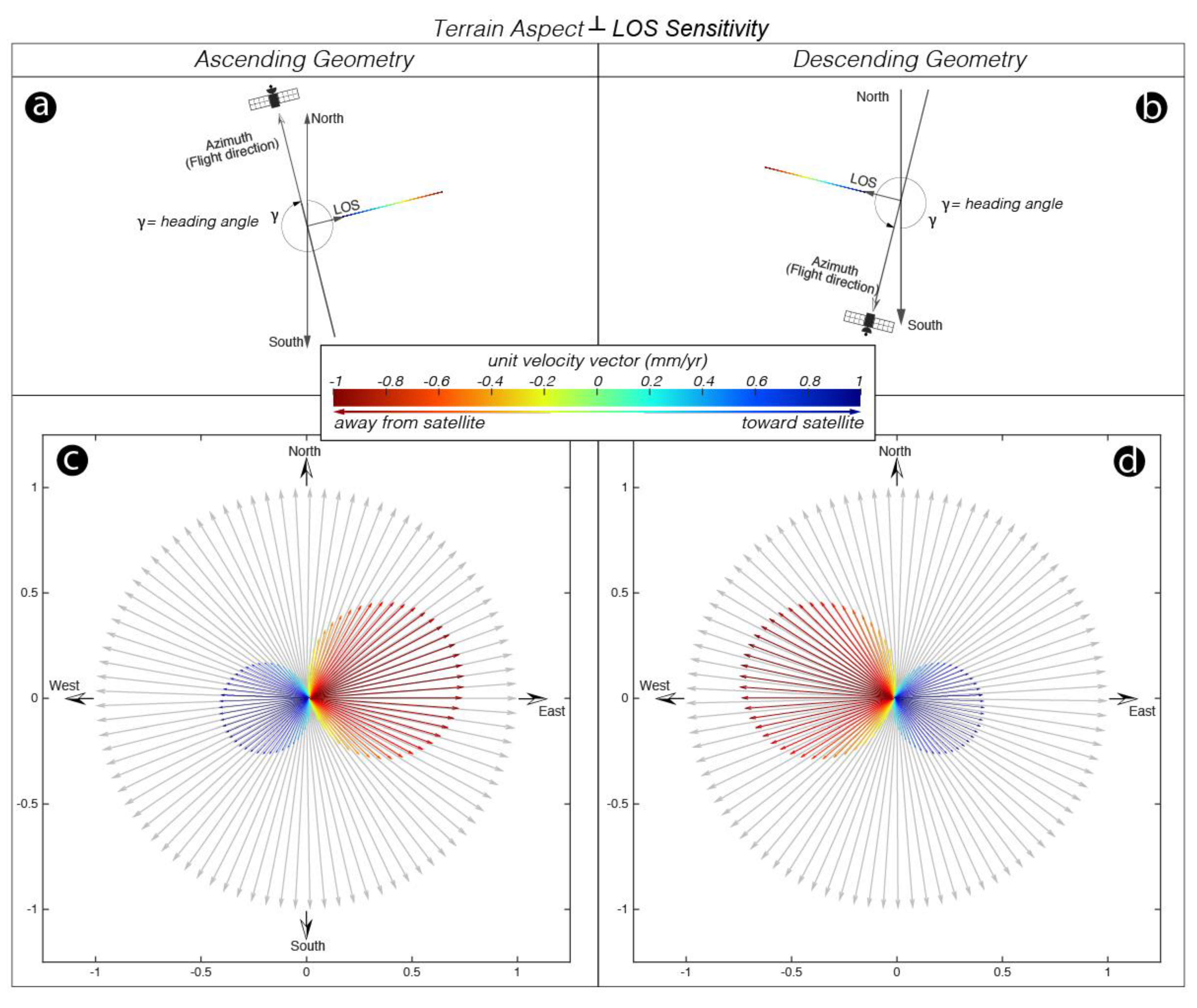
Impact of the Satellite Sensor Viewing Geometry on Monitoring Down-Slope Movement
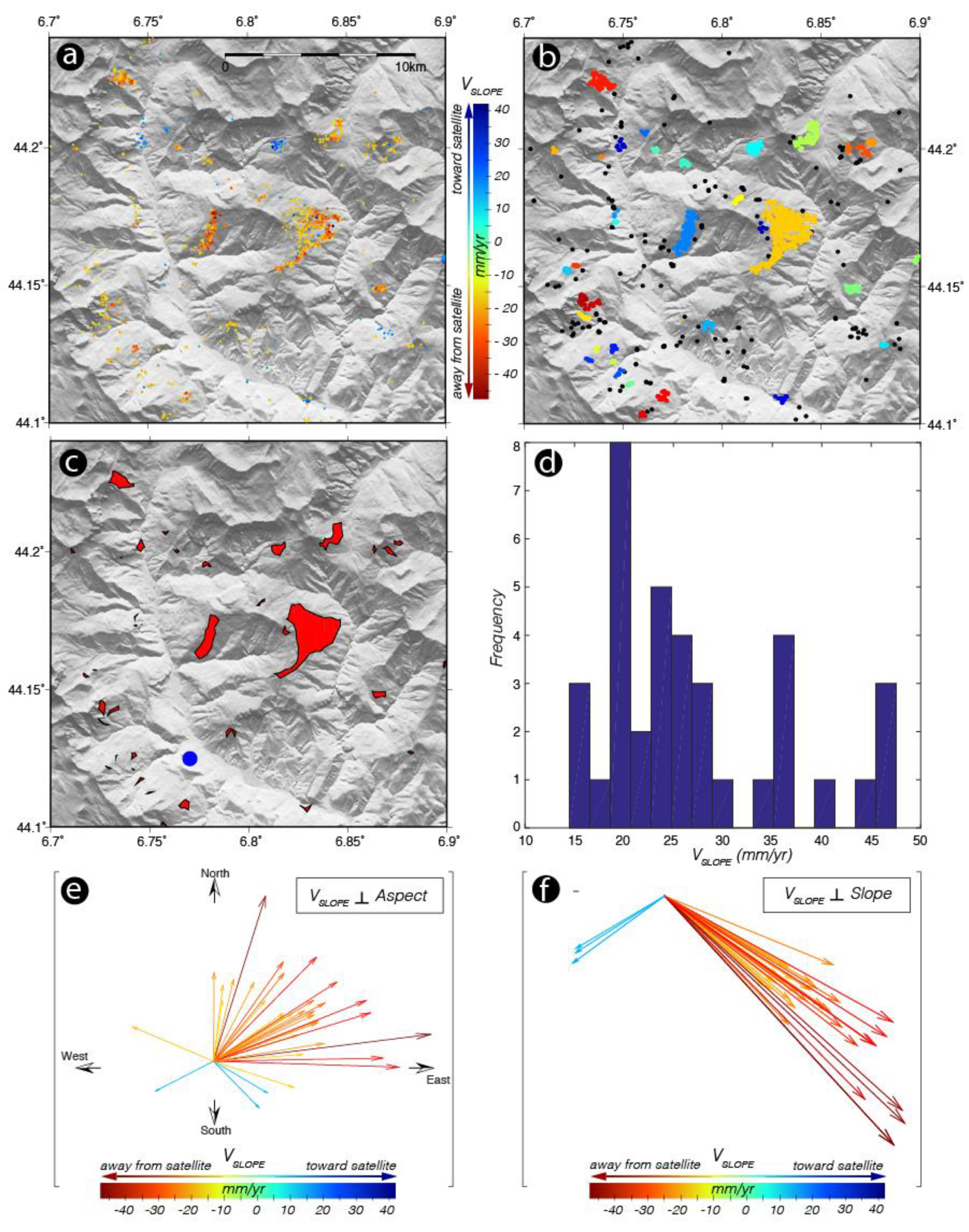
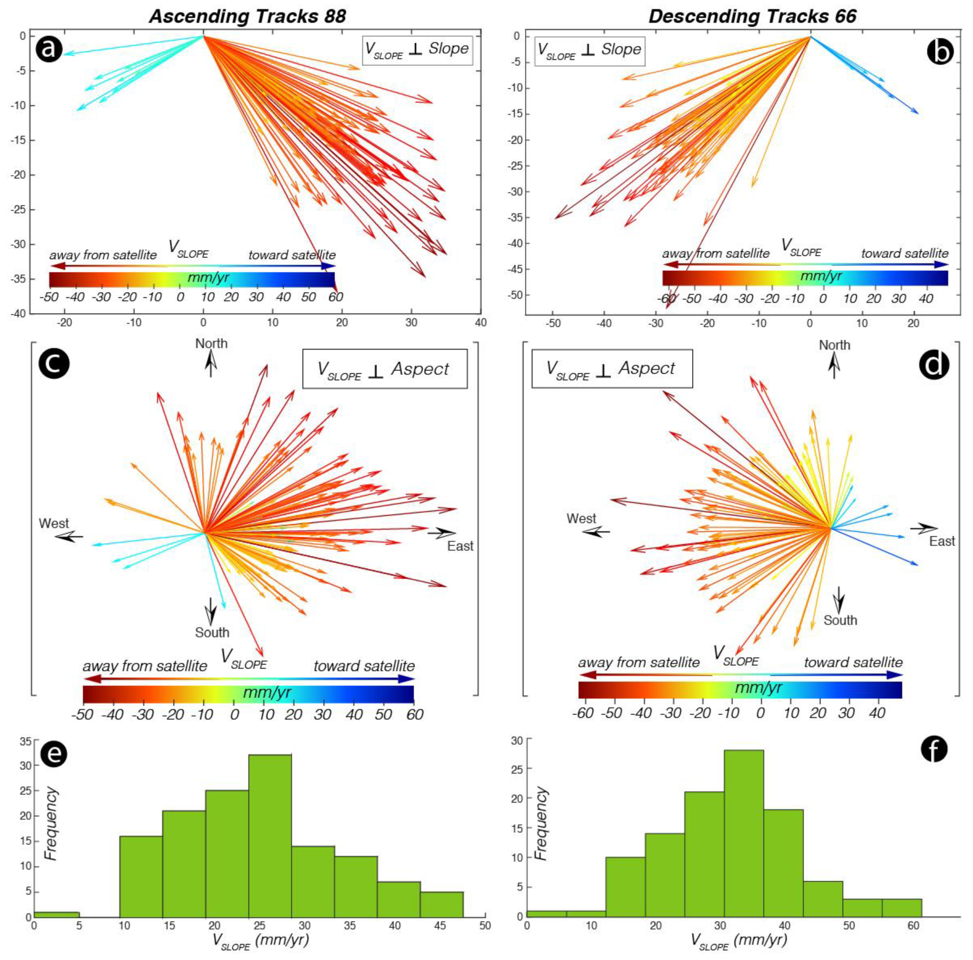
5. Results
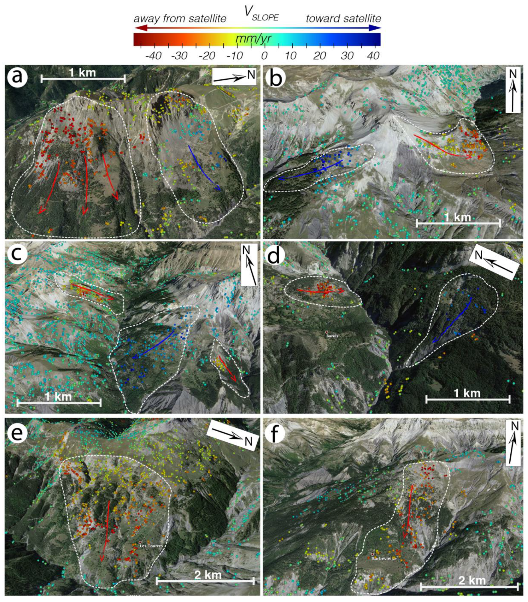
Landslide Identification Results
6. Conclusions
Author Contributions
Funding
Acknowledgments
Conflicts of Interest
References
- Cruden, D.M.; Varnes, D.J. Landslides: Investigation and Mitigation. Chapter 3-Landslide Types and Processes; Transportation Research Board Special Report; The National Academies of Sciences, Engineering, and Medicine: Washington, DC, USA, 1996; Volume 247. [Google Scholar]
- Delacourt, C.; Allemand, P.; Berthier, E.; Raucoules, D.; Casson, B.; Grandjean, P.; Varel, E. Remote-sensing techniques for analysing landslide kinematics: A review. Bull. Société Géologique Fr. 2007, 178, 89–100. [Google Scholar] [CrossRef]
- Van Westen, C.J.; Van Asch, T.W.; & Soeters, R. Landslide hazard and risk zonation—Why is it still so difficult? Bull. Eng. Geol. Environ. 2006, 65, 167–184. [Google Scholar] [CrossRef]
- Van Den Eeckhaut, M.; Hervás, J. Landslide inventories in Europe and policy recommendations for their interoperability and harmonization. JRC Sci. Policy Rep. 2012. [Google Scholar] [CrossRef]
- Cigna, F.; Bianchini, S.; Casagli, N. How to assess landslide activity and intensity with Persistent Scatterer Interferometry (PSI): The PSI-based matrix approach. Landslides 2013, 10, 267–283. [Google Scholar] [CrossRef]
- Aleotti, P.; Chowdhury, R. Landslide hazard assessment: Summary review and new perspectives. Bull. Eng. Geol. Environ. 1999, 58, 21–44. [Google Scholar] [CrossRef]
- Dai, F.C.; Lee, C.F.; Ngai, Y.Y. Landslide risk assessment and management: An overview. Eng. Geol. 2002, 64, 65–87. [Google Scholar] [CrossRef]
- Guzzetti, F.; Mondini, A.C.; Cardinali, M.; Fiorucci, F.; Santangelo, M.; Chang, K.T. Landslide inventory maps: New tools for an old problem. Earth Sci. Rev. 2012, 112, 42–66. [Google Scholar] [CrossRef]
- Burns, W.J.; Madin, I. Protocol for Inventory Mapping of Landslide Deposits from Light Detection and Ranging (LiDAR) Imagery Portland; Department of Geology and Mineral Industries: Oregon, OR, USA, 2009; pp. 1–30. [Google Scholar]
- Guzzetti, F.; Cardinali, M.; Reichenbach, P.; Carrara, A. Comparing Landslide Maps: A Case Study in the Upper Tiber River Basin, Central Italy. Environ. Manag. 2000, 25, 247–263. [Google Scholar] [CrossRef]
- Frangioni, S.; Bianchini, S.; Moretti, S. Geomatics, Natural Hazards and Risk. Landslide inventory updating by means of Persistent Scatterer Interferometry (PSI): The Setta basin (Italy) case study. Geomat. Nat. Hazards Risk 2014. [Google Scholar] [CrossRef]
- Malamud, B.D.; Turcotte, D.L.; Guzzetti, F.; Reichenbach, P. Landslide inventories and their statistical properties. Earth Surf. Process. Landf. 2004, 29, 687–711. [Google Scholar] [CrossRef]
- Brardinoni, F.; Slaymaker, O.; Hassan, M.A. Landslide inventory in a rugged forested watershed: A comparison between air-photo and field survey data. Geomorphology 2003, 54, 179–196. [Google Scholar] [CrossRef]
- Van Den Eeckhaut, M.; Poesen, J.; Verstraeten, G.; Vanacker, V.; Moeyersons, J.; Nyssen, J.; Van Beek, L.P.H. The effectiveness of hillshade maps and expert knowledge in mapping old deep-seated landslides. Geomorphology 2005, 67, 351–363. [Google Scholar] [CrossRef]
- Vietmeier, J.; Wagner, W.; Dikau, R. Monitoring moderate slope movements (landslides) in the southern French Alps using differential SAR interferometry. In Proceedings of the Fringe 1999 Workshop: Advancing ERS SAR Interferometry from Applications Towards Operations, Liège, Belgium, 10–12 November 1999; Volume 99, pp. 10–12. [Google Scholar]
- Catani, F.; Farina, P.; Moretti, S.; Nico, G.; Strozzi, T. On the application of SAR interferometry to geomorphological studies: Estimation of landform attributes and mass movements. Geomorphology 2005, 66, 119–131. [Google Scholar] [CrossRef]
- Strozzi, T.; Farina, P.; Corsini, A.; Ambrosi, C.; Thüring, M.; Zilger, J.; Werner, C. Survey and monitoring of landslide displacements by means of L-band satellite SAR interferometry. Landslides 2005, 2, 193–201. [Google Scholar] [CrossRef]
- Calabro, M.D.; Schmidt, D.A.; Roering, J.J. An examination of seasonal deformation at the Portuguese Bend landslide, southern California, using radar interferometry. J. Geophys. Res. Earth Surf. 2010, 115. [Google Scholar] [CrossRef]
- Schlögel, R.; Doubre, C.; Malet, J.P.; Masson, F. Landslide deformation monitoring with ALOS/PALSAR imagery: A D-InSAR geomorphological interpretation method. Geomorphology 2015, 231, 314–330. [Google Scholar] [CrossRef]
- Raucoules, D.; de Michele, M.; Aunay, B. Landslide displacement mapping based on ALOS-2/PALSAR-2 data using image correlation techniques and SAR interferometry: Application to the Hell-Bourg landslide (Salazie circle, La Réunion Island). Geocarto Int. 2020, 35, 113–127. [Google Scholar] [CrossRef]
- Berardino, P.; Fornaro, G.; Lanari, R.; Sansosti, E. A new algorithm for surface deformation monitoring based on small baseline differential SAR interferograms. IEEE Trans. Geosci. Remote Sens. 2002, 40, 2375–2383. [Google Scholar] [CrossRef]
- Lanari, R.; Mora, O.; Manunta, M.; Mallorquí, J.J.; Berardino, P.; Sansosti, E. A small-baseline approach for investigating deformations on full-resolution differential SAR interferograms. IEEE Trans. Geosci. Remote Sens. 2004, 42, 1377–1386. [Google Scholar] [CrossRef]
- Casu, F.; Manzo, M.; Lanari, R. A quantitative assessment of the SBAS algorithm performance for surface deformation retrieval from DInSAR data. Remote Sens. Environ. 2006, 102, 195–210. [Google Scholar] [CrossRef]
- Farina, P.; Colombo, D.; Fumagalli, A.; Marks, F.; Moretti, S. Permanent Scatterers for landslide investigations: Outcomes from the ESA-SLAM project. Eng. Geol. 2006, 88, 200–217. [Google Scholar] [CrossRef]
- Cascini, L.; Fornaro, G.; Peduto, D. Advanced low-and full-resolution DInSAR map generation for slow-moving landslide analysis at different scales. Eng. Geol. 2010, 112, 29–42. [Google Scholar] [CrossRef]
- Herrera, G.; Notti, D.; García-Davalillo, J.C.; Mora, O.; Cooksley, G.; Sánchez, M.; Crosetto, M. Analysis with C-and X-band satellite SAR data of the Portalet landslide area. Landslides 2011, 8, 195–206. [Google Scholar] [CrossRef]
- Righini, G.; Pancioli, V.; Casagli, N. Updating landslide inventory maps using Persistent Scatterer Interferometry (PSI). Int. J. Remote Sens. 2011, 33, 2068–2096. [Google Scholar] [CrossRef]
- Bovenga, F.; Wasowski, J.; Nitti, D.O.; Nutricato, R.; Chiaradia, M.T. Using COSMO/SkyMed X-band and ENVISAT C-band SAR interferometry for landslides analysis. Remote Sens. Environ. 2012, 119. [Google Scholar] [CrossRef]
- Tofani, V.; Raspini, F.; Catani, F.; & Casagli, N. Persistent Scatterer Interferometry (PSI) technique for landslide characterization and monitoring. Remote Sens. 2013, 5, 1045–1065. [Google Scholar] [CrossRef]
- Perissin, D.; Wang, T. Repeat-pass SAR interferometry with partial coherent targets. IEEE Trans. Geoscience Remote Sens. 2011, 50, 271–280. [Google Scholar] [CrossRef]
- Foumelis, M.; Raucoules, D.; Colas, B.; de Michele, M. On the effect of interferometric pairs selection for measuring fast moving landslides. In Proceedings of the International Geoscience and Remote Sensing Symposium (IGARSS 2019), Yokohama, Japan, 28 July–2 August 2019. [Google Scholar]
- Di Martire, D.; Tessitore, S.; Brancato, D.; Ciminelli, M.G.; Costabile, S.; Costantini, M.; Calcaterra, D. Landslide detection integrated system (LaDIS) based on in-situ and satellite SAR interferometry measurements. Catena 2016, 137, 406–421. [Google Scholar] [CrossRef]
- Refice, A.; Spalluto, L.; Bovenga, F.; Fiore, A.; Miccoli, M.N.; Muzzicato, P.; Pasquariello, G. Integration of persistent scatterer interferometry and ground data for landslide monitoring: The Pianello landslide (Bovino, Southern Italy). Landslides 2019, 16, 447–468. [Google Scholar] [CrossRef]
- Zhao, C.; Lu, Z.; Zhang, Q.; de La Fuente, J. Large-area landslide detection and monitoring with ALOS/PALSAR imagery data over Northern California and Southern Oregon, USA. Remote Sens. Environ. 2012, 124, 348–359. [Google Scholar] [CrossRef]
- Zhao, C.; Kang, Y.; Zhang, Q.; Lu, Z.; Li, B. Landslide identification and monitoring along the Jinsha River catchment (Wudongde reservoir area), China, using the InSAR method. Remote Sens. 2018, 10, 993. [Google Scholar] [CrossRef]
- Liu, X.; Zhao, C.; Zhang, Q.; Peng, J.; Zhu, W.; Lu, Z. Multi-temporal loess landslide inventory mapping with C-, X-and L-band SAR datasets—A case study of Heifangtai Loess Landslides, China. Remote Sens. 2018, 10, 1756. [Google Scholar] [CrossRef]
- Meisina, C.; Zucca, F.; Notti, D.; Colombo, A.; Cucchi, A.; Savio, G.; Giannico, C.; Bianchi, M. Geological interpretation of PS InSAR data at regional scale. Sensors 2008, 8, 7469–7492. [Google Scholar] [CrossRef]
- Barra, A.; Solari, L.; Béjar-Pizarro, M.; Monserrat, O.; Bianchini, S.; Herrera, G.; Ligüerzana, S. A methodology to detect and update active deformation areas based on sentinel-1 SAR images. Remote Sens. 2017, 9, 1002. [Google Scholar] [CrossRef]
- Solari, L.; Bianchini, S.; Franceschini, R.; Barra, A.; Monserrat, O.; Thuegaz, P.; Catani, F. Satellite interferometric data for landslide intensity evaluation in mountainous regions. Int. J. Appl. Earth Obs. Geoinf. 2020, 87, 102028. [Google Scholar] [CrossRef]
- Solari, L.; Barra, A.; Herrera, G.; Bianchini, S.; Monserrat, O.; Béjar-Pizarro, M.; Moretti, S. Fast detection of ground motions on vulnerable elements using Sentinel-1 InSAR data. Geomat. Nat. Hazards Risk 2018, 9, 152–174. [Google Scholar] [CrossRef]
- Tomás, R.; Pagán, J.I.; Navarro, J.A.; Cano, M.; Pastor, J.L.; Riquelme, A.; Lopez-Sanchez, J.M. Semi-automatic identification and pre-screening of geological–geotechnical deformational processes using persistent scatterer interferometry datasets. Remote Sens. 2019, 11, 1675. [Google Scholar] [CrossRef]
- Bianchini, S.; Cigna, F.; Righini, G.; Proietti, C.; Casagli, N. Landslide hotspot mapping by means of persistent scatterer interferometry. Environ. Earth Sci. 2012. [Google Scholar] [CrossRef]
- Bianchini, S.; Herrera, G.; Mateos, R.M.; Notti, D.; Garcia, I.; Mora, O.; Moretti, S. Landslide activity maps generation by means of persistent scatterer interferometry. Remote Sens. 2013, 5, 6198–6222. [Google Scholar] [CrossRef]
- Herrera, G.; Gutiérrez, F.; García-Davalillo, J.C.; Guerrero, J.; Notti, D.; Galve, J.P.; Cooksley, G. Multi-sensor advanced DInSAR monitoring of very slow landslides: The Tena Valley case study (Central Spanish Pyrenees). Remote Sens. Environ. 2013, 128, 31–43. [Google Scholar] [CrossRef]
- Notti, D.; Herrera, G.; Bianchini, S.; Meisina, C.; García-Davalillo, J.C.; Zucca, F. A methodology for improving landslide psi data analysis. Int. J. Remote Sens. 2014, 35, 2186–2214. [Google Scholar] [CrossRef]
- Schlögel, R.; Malet, J.P.; Doubre, C.; Lebourg, T. Structural control on the kinematics of the deep-seated La Clapière landslide revealed by L-band InSAR observations. Landslides 2016, 13, 1005–1018. [Google Scholar] [CrossRef]
- Squarzoni, C.; Delacourt, C.; Allemand, P. Nine years of spatial and temporal evolution of the La Valette landslide observed by SAR interferometry. Eng. Geol. 2003, 68, 53–66. [Google Scholar] [CrossRef]
- Leprince, S.; Berthier, E.; Ayoub, F.; Delacourt, C.; Avouac, J.P. Monitoring earth surface dynamics with optical imagery. Eos Trans. Am. Geophys. Union 2008, 89, 1–2. [Google Scholar] [CrossRef]
- Raucoules, D.; De Michele, M.; Malet, J.P.; Ulrich, P. Time-variable 3D ground displacements from high-resolution synthetic aperture radar (SAR). Application to La Valette landslide (South French Alps). Remote Sens. Environ. 2013, 139, 198–204. [Google Scholar] [CrossRef]
- Desrues, M.; Lacroix, P.; Brenguier, O. Satellite Pre-Failure Detection and In Situ Monitoring of the Landslide of the Tunnel du Chambon, French Alps. Geosciences 2019, 9, 313. [Google Scholar] [CrossRef]
- Fernandez, P.; Whitworth, M. A new technique for the detection of large scale landslides in glacio-lacustrine deposits using image correlation based upon aerial imagery: A case study from the French Alps. Int. J. Appl. Earth Obs. Geoinf. 2016, 52, 1–11. [Google Scholar] [CrossRef][Green Version]
- Lacroix, P.; Bièvre, G.; Pathier, E.; Kniess, U.; Jongmans, D. Use of Sentinel-2 images for the detection of precursory motions before landslide failures. Remote Sens. Environ. 2018, 215, 507–516. [Google Scholar] [CrossRef]
- Walter, M.; Niethammer, U.; Rothmund, S.; Joswig, M. Joint analysis of the Super-Sauze (French Alps) mudslide by nanoseismic monitoring and UAV-based remote sensing. First Break 2009, 27. [Google Scholar]
- Mirzaee, S.; Motagh, M.; Akbari, B.; Wetzel, H.U.; Roessner, S. Evaluating Three Insar Time-Series Methods to Assess Creep Motion, Case Study: Masouleh Landslide In North Iran. Isprs Annals of Photogrammetry. Remote Sens. Spat. Inf. Sci. 2017, 4, 223–228. [Google Scholar] [CrossRef]
- Sandwell, D.; Mellors, R.; Tong, X.; Wei, M.; Wessel, P. Open Radar Interferometry Software for Mapping Surface Deformation. Eos Trans. AGU 2011, 92, 234. [Google Scholar] [CrossRef]
- Farr, T.; Rosen, P.; Caro, E.; Crippen, R.; Duren, R.; Hensley, S.; Alsdorf, D. The shuttle radar topography mission. Rev. Geophys. 2007, 45. [Google Scholar] [CrossRef]
- Hooper, A. A Multi-temporal InSAR method incorporating both persistent scatterer and small baseline approaches. Geophys. Res. Lett. 2008, 35. [Google Scholar] [CrossRef]
- Hooper, A.; Bekaert, D.; Spaans, K.; Arıkan, M. Recent advances in SAR interferometry time series analysis for measuring crustal deformation. Tectonophysics 2011, 514, 1–13. [Google Scholar] [CrossRef]
- Ferretti, A.; Prati, C.; Rocca, F. Permanent scatterers in SAR interferometry. IEEE Trans. Geosci. Remote Sens. 2001, 39, 8–20. [Google Scholar] [CrossRef]
- Bekaert, D.P.S.; Walters, R.J.; Wright, T.J.; Hooper, A.J.; Parker, D.J. Statistical comparison of InSAR tropospheric correction techniques. Remote Sens. Environ. 2015, 170, 40–47. [Google Scholar] [CrossRef]
- Dee, D.P.; Uppala, S.M.; Simmons, A.J.; Berrisford, P.; Poli, P.; Kobayashi, S.; Andrea, U. The ERA-Interim reanalysis: Configuration and performance of the data assimilation system. Q. J. R. Meteorol. Soc. 2011, 137, 553–597. [Google Scholar] [CrossRef]
- Li, Y.; Mo, P. A unified landslide classification system for loess slopes: A critical review. Geomorphology 2019. [Google Scholar] [CrossRef]
- Hanssen, R.F. Radar Interferometry: Data Interpretation and Error Analysis; Kluwer Academic Publishers: Dordrecht, The Netherlans, 2001. [Google Scholar]
- Alatza, S.; Papoutsis, I.; Paradissis, D.; Kontoes, C.; Papadopoulos, G.A. Multi-Temporal InSAR Analysis for Monitoring Ground Deformation in Amorgos Island, Greece. Sensors 2020, 20, 338. [Google Scholar] [CrossRef]
- Colesanti, C.; Wasowski, J. Investigating landslides with space-borne Synthetic Aperture Radar (SAR) Interferometry. Eng. Geol. 2006, 88, 173–199. [Google Scholar] [CrossRef]
- Del Soldato, M.; Solari, L.; Poggi, F.; Raspini, F.; Tomás, R.; Fanti, R.; & Casagli, N. Landslide-Induced Damage Probability Estimation Coupling InSAR and Field Survey Data by Fragility Curves. Remote Sens. 2019, 11, 1486. [Google Scholar] [CrossRef]
- Kalia, A.C. Classification of landslide activity on a regional scale using persistent scatterer interferometry at the moselle valley (Germany). Remote Sens. 2018, 10, 1880. [Google Scholar] [CrossRef]
- Béjar-Pizarro, M.; Notti, D.; Mateos, R.M.; Ezquerro, P.; Centolanza, G.; Herrera, G.; Fernández, J. Mapping vulnerable urban areas affected by slow-moving landslides using Sentinel-1 InSAR data. Remote Sens. 2017, 9, 876. [Google Scholar] [CrossRef]
- Bardi, F.; Raspini, F.; Ciampalini, A.; Kristensen, L.; Rouyet, L.; Lauknes, T.R.; Casagli, N. Space-borne and ground-based InSAR data integration: The Åknes test site. Remote Sens. 2016, 8, 237. [Google Scholar] [CrossRef]
- Ester, M.; Kriegel, H.P.; Sander, J.; Xu, X. A Density-Based Algorithm for Discovering Clusters in Large Spatial Databases with Noise. In Proceedings of the 2nd International Conference on Knowledge Discovery and Data Mining, Portland, OR, USA, 2–4 August 1996; AAAI Press: City of Menlo Park, CA, USA, 1996; pp. 226–231. [Google Scholar]
- Schubert, E.; Sander, J.; Ester, M.; Kriegel, H.P.; Xu, X. DBSCAN revisited, revisited: Why and how you should (still) use DBSCAN. ACM Trans. Database Syst. 2017, 42, 19. [Google Scholar] [CrossRef]
- Xuejun, L.; Lu, B. Accuracy Assessment of DEM Slope Algorithms Related to Spatial Autocorrelation of DEM Errors. In Advances in Digital Terrain Analysis. Lecture Notes in Geoinformation and Cartography; Zhou, Q., Lees, B., Tang, G., Eds.; Springer: Berlin/Heidelberg, Germany, 2008. [Google Scholar]
- Carlà, T.; Intrieri, E.; Raspini, F.; Bardi, F.; Farina, P.; Ferretti, A.; Casagli, N. Perspectives on the prediction of catastrophic slope failures from satellite InSAR. Sci. Rep. 2019, 9, 14137. [Google Scholar] [CrossRef] [PubMed]
- Fuhrmann, T.; Garthwaite, M.C. Resolving three-dimensional surface motion with InSAR: Constraints from multi-geometry data fusion. Remote Sens. 2019, 11, 241. [Google Scholar] [CrossRef]


| Track | Sensor | Geometry | Time Interval | Incidence Angle (°) | Interferograms Used | Density 2 (PS/km2) |
|---|---|---|---|---|---|---|
| T88 | SENTINEL 1 | Ascending | 2016–2019 | 30.5~35.5 | 58 | ~53 |
| T66 | SENTINEL 1 | Descending | 2015–2019 | 40.5~45.5 | 50 | ~24 |
© 2020 by the authors. Licensee MDPI, Basel, Switzerland. This article is an open access article distributed under the terms and conditions of the Creative Commons Attribution (CC BY) license (http://creativecommons.org/licenses/by/4.0/).
Share and Cite
Aslan, G.; Foumelis, M.; Raucoules, D.; De Michele, M.; Bernardie, S.; Cakir, Z. Landslide Mapping and Monitoring Using Persistent Scatterer Interferometry (PSI) Technique in the French Alps. Remote Sens. 2020, 12, 1305. https://doi.org/10.3390/rs12081305
Aslan G, Foumelis M, Raucoules D, De Michele M, Bernardie S, Cakir Z. Landslide Mapping and Monitoring Using Persistent Scatterer Interferometry (PSI) Technique in the French Alps. Remote Sensing. 2020; 12(8):1305. https://doi.org/10.3390/rs12081305
Chicago/Turabian StyleAslan, Gokhan, Michael Foumelis, Daniel Raucoules, Marcello De Michele, Severine Bernardie, and Ziyadin Cakir. 2020. "Landslide Mapping and Monitoring Using Persistent Scatterer Interferometry (PSI) Technique in the French Alps" Remote Sensing 12, no. 8: 1305. https://doi.org/10.3390/rs12081305
APA StyleAslan, G., Foumelis, M., Raucoules, D., De Michele, M., Bernardie, S., & Cakir, Z. (2020). Landslide Mapping and Monitoring Using Persistent Scatterer Interferometry (PSI) Technique in the French Alps. Remote Sensing, 12(8), 1305. https://doi.org/10.3390/rs12081305