Abstract
Analysis of urban dynamics is a pivotal step towards understanding landscape changes and developing scientifically sound urban management strategies. Delineating the patterns and processes shaping the evolution of urban regions is an essential part of this step. Utilizing remote-sensing techniques and Geographic Information System (GIS) tools, we performed an integrated analysis on urban expansion in Srinagar city and surrounding areas from 1999 to 2017 at multiple scales in order to assist urban planning initiatives. To capture various spatial indicators of expansion, we analysed (i) land use/land cover (LULC) changes, (ii) rate and intensity of changes to built-up areas, (iii) spatial differentiation in landscape metrics (at 500, 1000 and 2000 m cell-size), and (iv) growth type of the urban expansion. Global Moran’s I statistics and local indicators of spatial association (LISA) were also employed to identify hotspots of change in landscape structure. Our methodology utilizes a range of geovisualization tools which are capable of appropriately addressing various elements required for strategic planning in growing cities. The results highlight aggregation and homogenization of the urban core as well as irregularity and fragmentation in its periphery. A combination of spatial metrics and growth type analysis supports the supposition that there is a continuum in the diffusion-coalescence process. This allows us to extend our understanding of urban growth theory and to report deviations from accepted stages of growth. As our results show, each dominating growth phase of the city—both diffusion (1999) and coalescence (2009 and 2017)—is interspersed with features from the other type. An improved understanding of spatial differentiation and the identification of hotspots can serve to make urban planning more tailored to such local conditions. An important insight derived from the results is the applicability of remote-sensing data in urban planning measures and the usefulness of freely available medium resolution data in gaining a comprehensive understanding of the evolution of cities.
1. Introduction
Globally, urban dynamics and their associated impacts have led to changes in the basic structure and function of ecosystems [1,2]. Urban transformations are multidimensional changes that are both dynamic and non-linear [3]. These changes are known to have transformed the immediate urban environment and continuously lead to a transition in other ecosystems around the world. Thus, cities have turned into the nodal points of global change. However, in recent times, the majority of urban growth has shifted from the developed to the developing world [4]. Nations experiencing rapid economic transformation, such as India and China, are the hotspots of this new urban growth [5,6]. In India in particular, existing population pressure coupled with other factors, such as governance priorities, socio-economic conditions, and the partial enforcement of land-use policy, has led to an extensive unplanned expansion of urban areas. India, home to 1 in 10 of the world’s urban residents [7], currently possesses huge potential to shape the urban sustainability narrative of the world. Unplanned and unmonitored urban growth presents a major hindrance to achieving sustainable development, as the tools to steer, monitor and measure its impacts are lacking [8]. With increasing demographic pressure and the complexity of urban systems, urban local governance bodies require tools that are easily adaptable and integrated into the existing framework of implementing policies. Applied remote sensing in conjunction with a Geographic Information System (GIS) provides a much needed leap in technology to identify the patterns and processes of expansion, and to record and map them for planning purposes. Such information, when combined with demographic and economics-based measures, has the potential to provide policy makers with more scientific decision-making capacity.
The sheer complexity and the dynamic trajectories of individual urban ecosystems are a major factor in bringing uncertainty into management strategies [9]. Most prominently from a spatial perspective, high interconnectivity, heterogeneity, and the transition probability of various spatial units contribute to this complexity [10]. A result of this increased urban complexity is its ability to influence ecological processes, ecosystem services, and the availability of natural resources for sustainable use [11]. Urban form, or morphology, a result of the path-dependent urbanization process, in turn provides a basis to understand the consequences of ecological, socio-economic, governance, and planning processes which ultimately shape the urban region. Due to efforts to decipher urban complexity and morphology, the growth of urban research has gained momentum in the past decades [12,13]. Understanding spatial patterns beyond the one-dimensional measure of land-use change has been a major focus of research to improve urban planning inputs [14]. Remote sensing and GIS techniques have been found to contribute very effectively towards capturing the spatial and temporal heterogeneity of land-use and land-cover (LULC) patterns in and around urban areas [15].
The ways in which the mosaic of LULC types are characterized to determine attributes such as their complexity, configuration, composition, shape, and irregularity have been studied widely in order to shed light on urban landscape dynamics [16,17,18]. Spatial metrics or landscape metrics, originating from the field of landscape ecology, are important and reliable tools utilized in this regard [19,20]. Most of the studies have focused on the analysis of multi-temporal sprawl patterns, providing measures of overall landscape metrics for a city or directional sections of a city and its surrounding areas [21,22,23,24]. However, this leads to a generalization of variations within the urban landscape and thus requires more distinct measurements which can capture spatial variations [18,25], a step with practical applicability in urban planning. Variations in landscape metrics are a spatially conditioned process, i.e., values in one location are related to nearby values, depending on the scale of observation. Thus, consideration of scale effects is important because they are more prominent in a heterogeneous landscape like urban areas [26]. To a great extent, landscape transformation processes are affected by processes in other locations, and thus the use of tools to measure spatial relationships is equally important [25]. Studying spatial relationships between the elements of a landscape arranged in different sizes and shapes provides the opportunity to delineate the patterns and processes shaping urban ecosystems. However, landscape metrics on their own do not provide all the necessary information on landscape structure, as they do not address measures of rate and intensity. Measuring changes over time in the urban area is an important part of understanding periods of growth, push-backs and stagnation phases [15,27]. Growth type assessment is an important step in identifying the spatial heterogeneity present in the evolution of an urban region, capable of depicting the processes through which urban growth has been shaped. Most studies refer to three growth type categories—infilling, outlying, and edge-expansion [28,29,30]. Growth types develop as a result of specific growth processes, and their analysis is a valuable contribution to urban planning and management. It allows a spatial identification of regions experiencing process-driven urban expansion and thus holds the key to countering the ensuing ecological consequences [31].
The rapid rate of urbanization, especially in the developing world, creates a challenging environment for urban planning and management. Urban areas located in valleys or basins are additionally subject to topographic constraints. The purpose of this study is to shed light on the urban dynamics of the largest Indian urban settlement in the Himalaya, Srinagar, and to emphasise the role of various mapping and monitoring tools and techniques used to delineate possible implications for future land-use planning. Another important contribution of this study is to address the scale-dependent interplay of spatial metrics and to develop a deeper understanding of the urban growth theory proposed by Dietzel et al., (2005) [32]. Previous studies have affirmed this alternating pattern of growth between diffusion and coalescence [33,34,35] while others have reported a transition phase from diffusion to coalescence [36,37]. However, literature on mountain cities remains fairly unexplored. Previous studies on cities like Srinagar have focused on urban sprawl [38] and land transformations [39], highlighting the unplanned nature of the city expansion and the resulting disproportionate distributions of resources. Patterns indicate a rapid increase in built-up areas and existing spatial variations in growth dominated by the edge-expansion category. However, a major gap in knowledge results from a lack of understanding about the landscape characteristics of built-up areas. Landscape characteristics measured through spatial indicators like landscape metrics provide detailed and varied information on the geometric patterns of built-up areas and can significantly improve our understanding of pattern-based processes such as fragmentation and irregularity. Beyond this, it is necessary to gain a comprehensive understanding of different indicators of urban growth at different spatio-temporal levels. To fill the existing knowledge gaps and improve the methodological approach in assessing urban dynamics, our objectives are to: (1) quantify and characterize the urban growth of the city and its environs; (2) understand the variations in the evolution of this urbanization using spatial metrics at different spatiotemporal scales and identify specific clusters of urban growth; and (3) determine the typology of urban growth in different parts of the city and its surroundings.
2. Materials and Methods
2.1. Study Area
Srinagar, the only million-plus city and the largest urban settlement in the Himalayan mountain chain, is located in the Kashmir valley of Northern India. It represents an active region of urban growth and is the centre of political, social, and economic exchange of the former state of Jammu and Kashmir (J & K) (now a central administered region). Srinagar city covers an area of 245 km2 and is divided into 69 administrative wards. According to the census in 2011, the city had a population of 1,180,570 inhabitants. To capture both regional and city-level urbanization, the study area encompasses an area of 1886 km2 (Figure 1) and includes Srinagar city and its surrounding areas at a distance of 25 km from the centre.
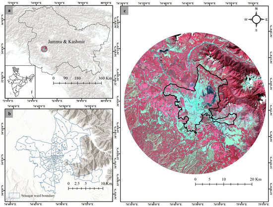
Figure 1.
Location of the study area Srinagar, India: (a) geographical location of study area in Jammu and Kashmir; (b) administrative wards of Srinagar city (see supplementary Table S1 for ward names); (c) satellite image of the study area.
At an average altitude of 1580 m, the physio-geographic layout of the area reflects its spatial heterogeneity, with vast agricultural fields in the south and western part as well as high elevation mountains in the north-eastern and eastern direction. These geographic features have significantly shaped the expansion of the settlement, leading to vast urban growth towards the plains and more restricted growth towards the mountains. The river Jhelum and Dal lake both play an important role as tourist recreation sites, ecosystem service providers and income generators for the local population. The city is also known for its diverse parks and green spaces, frequently accessed by residents and tourists. Being exposed to the highest (very severe) intensity seismic zone, the city and its surroundings have a considerable vulnerability to earthquakes, while flooding is another natural hazard.
2.2. Data Processing and Land-Use and Land-Cover (LULC) Classification
Urban dynamics in the study area were analysed using multi-spectral satellite images covering almost two decades at three points in time, i.e., 1999, 2009 and 2017. The images were obtained from Landsat 5 (TM) and 8 (OLI/TIRS) satellites provided by USGS (United States Geological Survey) (http://earthexplorer.usgs.gov/) at a spatial resolution of 30 m. Table S2 (see supplementary data) provides further details on the acquisition dates, sensors and path/row of the images obtained.
Prior to generating LULC maps, the images were processed for atmospheric correction using the fast line-of-sight atmospheric analysis of hypercubes (FLAASH) algorithm embedded in the Environment for Visualizing Images (ENVI) software v.4.7 in order to minimize the atmospheric effects. To classify the images, a supervised classification technique was applied using the maximum likelihood classifier (MLC), which is based on the similarity of spectral signatures. However, owing to the high spatial heterogeneity that is inherent to urban areas, the spatial resolution of Landsat images is not sufficient for all processes of spatial analysis, meaning that spectral signatures may be misclassified. For this reason, Google Earth images were used additionally to complement the training sample generation (Figure 2a). Each satellite image was classified into fourteen LULC classes, i.e., built-up dense, built-up sparse, fallow land, agriculture, forest, hilly vegetation, open land, bare mountain, barren, marshy vegetation, wetland, sand, river, and cloud (see supplementary data Table S3). The established nature of certain classes, such as bare mountain, hilly vegetation, cloud and sand, helped in classification as although not part of the main focus area of study they were essential to include as they covered a significant part of the overall study area. As the main focus of this study was on the built-up areas, two different classes were extracted that were based on the spectral differences and established LULC features in the urban region (see supplementary data Table S3).

Figure 2.
Methodological framework showing the major steps involved in the study: (a) data pre-processing and land-use and land-cover (LULC) classification, (b) LULC analysis, and (c) spatial pattern-process analysis.
The study area was divided into two sections: the city area (CA) enclosing the administrative area of the city, and the outer zone (OZ), the area surrounding the city from its boundary to a distance of 25 km from its centre (Figure 2b). Post-classification refinement was undertaken to remove singular LULC pixels and to reduce misclassification errors. Singular pixels were corrected using majority analysis with a 5 × 5 moving window. Owing to spectral similarity with built-up categories, bare mountainous slopes were carefully reclassified. Ancillary information such as the DEM (digital elevation model) obtained from ASTER (Advanced Spaceborne Thermal Emission and Reflection Radiometer) satellite sensors for the year 2011 was utilized to assist this process, and also to differentiate hilly vegetation from other vegetation classes based on elevation.
The accuracy assessment was carried out using bootstrapping technique that remove any human bias in the selection of sample pixels. A stratified random sampling technique was employed to obtain testing pixels for each class, collected using probability proportional to size (PPS) sampling (see supplementary data Table S4 for the number of reference sites associated with each class). Using the bootstrapping technique, 800 randomly generated testing pixels were subjected to 100 iterations without replacement. An R algorithm was employed to calculate user’s accuracy (UA), producer’s accuracy (PA), overall accuracy (OA) and kappa (K) statistics generated by the error matrix [40]. The mean value of all four parameters obtained from 100 iterations was considered as the final measure of the accuracy assessment.
2.3. Spatial Pattern-Process Analysis
To understand the complex relationship between landscape patterns and co-existing change processes driven by the patterns themselves, we followed three paths of spatial analysis (Figure 2c): (1) built-up change analysis, (2) landscape metrics analysis, and (3) growth pattern analysis. In the built-up change analysis, we quantified the urban expansion rate and intensity of urban growth, allowing simpler conclusions on the absolute change of the built-up area. In the landscape metrics analysis, we computed landscape metrics at differential spatiotemporal scales, i.e., 500 500 m, 1000 1000 m, and 2000 2000 m for the years 1999, 2009 and 2017 in order to determine the composition and configuration of the built-up area. Since the main focus in this part was on general trends of urban dynamics with respect to landscape metrics, the two classes dense and sparse built-up are combined to form a single built-up class. Thus, for each cell of the respective size, we computed the selected landscape metrics of this combined built-up class and analysed it further. As landscape metrics are known to be spatially dependent and to change across spatial resolutions, we calculated all the values at a spatial resolution of 30 m. With respect to this resolution, the selected cell sizes captured variation in the geometric values of the landscape metrics and allowed a determination of scale which captures the heterogeneity in the study area.
In the growth type analysis, we identified three different urban growth types across the city (infilling, edge-expansion and outlying). This integrated methodology helped us in capturing the structural changes in built-up patterns and enabled us to utilize an innovative way of visualizing localized information in different parts of the city. By focusing on more than one parameter of built-up area change, this methodology makes it possible to carry out a comprehensive analysis of urban dynamics, which is a key indicator for urban planners. Detailed analysis of spatial variation in landscape metrics and growth type is an essential step towards visualizing urban dynamics at the local level. The analytical inferences also contribute towards discussion of the phases of diffusion and coalescence in the context of the urban growth theory proposed by Dietzel et al., 2005 [34].
2.3.1. Measuring Expansion Rate and Intensity
To quantify the magnitude of urban expansion and understand spatial dynamics, two key indices, the urban expansion rate (Uer) and urban expansion intensity (Uei), are computed [15,41,42]. Uer quantifies change in the built-up areas (combined built-up class) as a percentage of total urban growth in the given interval (Equation (1)). This measure can provide direct evidence of demographic pressure and/or governance implications for the land system and helps to evaluate a direct footprint of urbanization [43]. Uei quantifies the change in built-up categories (combined built-up class) between different given points in time as a percentage of the total area in the selected land unit (Equation (2)). To visualize and comprehend urban dynamics at high spatial resolution, the ward level, which is the smallest administrative unit in India, was taken as the relevant land unit to compute Uer and Uei.
For each ward, respective indices were calculated using the following formulae:
where, and is the built-up area at time t + i and i respectively, and t is the interval between given points in time (in years). denotes the change in built-up area at time i, and is the total area of the land unit.
2.3.2. Multi-Scale Landscape Metrics Analysis
The analysis of landscape composition (a measure of the quantity - abundance, diversity, patch density etc. of a particular class without considering its spatial character) and configuration (a measure of the spatial character—shape complexity, nearest neighbour distance, arrangement etc.—of a particular class) is an important aspect when studying urban dynamics. Spatial heterogeneity of the landscape plays an important role in transition phases of ecological features [44]. Landscape metrics help to characterize the morphological regularities of a landscape by effectively characterizing the geometrical variation [45]. However, spatial heterogeneity at different spatiotemporal scales provides a higher or lower aggregation of information about a landscape due to the scale-dependent nature of cell-sizes [26]. Selected spatial metrics were analysed on three different scales, namely, 500 500 m, 1000 1000 m, and 2000 2000 m. Unlike other studies, the selection of these sizes makes it possible to test intermediate cell sizes [18,25].
To capture the spatial heterogeneity and derive the inner construct of feature characteristics, four spatial metrics were selected based on the objectives of the study and literature review. Many previous studies have proposed and selected a similar set of spatial metrics capable of measuring the dynamics of urban growth [46,47]. We chose a core set of four class-level metrics, namely, largest patch index (LPI), largest shape index (LSI), area-weighted mean patch fractal dimension (AWMPFD), and aggregation index (AI) (Table 1) based on their ability to highlight the composition and configuration of the landscape studied. As most studies lack spatial differentiation of landscape metrics, we have also analysed three commonly used landscape metrics, namely, number of patches (NP), Euclidean nearest-neighbour distance mean (ENNMN) [48] and patch density (PD). These single-value metrics for the whole study area would enable comparison with other studies and discussion of urban growth theory in general.

Table 1.
List and definition of applied spatial metrics in the study, (after McGarigal and Marks, 1995; McGarigal, 2015) [49,50].
LPI measures the dominance of urban patches and thus their composition. LSI, AWMPFD, and AI, measure the configuration of this urban landscape by delineating the complexity, fragmentation, and contiguity of urban patches [16,17]. To compute these metrics, FRAGSTATS, version 4.2 [49] was used. Prior to this, FISHNET (grid) of different sizes were generated (for LPI, LSI, AWMPFD and AI) in ArcGIS 10.7. Following this, batch clipping was performed to generate individual cells of specified size from each classified image using the model maker. Each grid size, i.e., 500 m, 1000 m and 2000 m generated 7717, 1974 and 518 individual grids, respectively, for each year. These grids were used in FRAGSTATS version 4.2 to compute the selected spatial metrics. The output was generated per grid cell with a resultant metrics value for each specified cell size.
2.3.3. Growth Type Analysis
Analysis of urban growth types, wherein each new urban patch is categorized into one of the recognized growth types, provides a deeper understanding of the landscape transformation processes [30]. Forman (1995) [51] classified three distinct growth types: infilling, outlying and edge-expansion. A quantitative method to extract such growth types was initiated by Wilson et al., 2003 [30] followed by Liu et al., 2010 [36] and Xu et al., 2007 [35]. These spatial patterns of growth are based on the urban expansion of the newer patch with respect to the older one. To extract this relation, the landscape expansion index (LEI) was calculated [36]. First, we performed a change detection analysis to identify old and new patches among the study years. The classes identified thus were re-coded to form three new classes: old, new and non-built up. These classes were converted to a polygon shapefile and used as input into the LEI tool box [36]. For each newly developed patch, LEI is computed as a ratio of the length of common edge () (old and new patch shares) to the total perimeter of the new patch ( (Equation (3)). The value of each new patch lies between 0 and 100.
Based on the LEI value(s), all the patches were classified into either of the three growth types using simple heuristic rules:
- (1)
- Infilling growth type: a new urban patch is surrounded by at least 50% of existing urban patches i.e., 50 < LEI .
- (2)
- Edge-expansion type: a new urban patch is surrounded by less than 50% of existing urban patches i.e., 0 < LEI 50.
- (3)
- Outlying growth type: a new urban patch is not surrounded by any existing urban patch i.e., LEI = 0
The defined growth types can also be related to the growth phases the city undergoes, in conjunction with trends in various spatial metrics.
2.4. Geospatial Statistical Analysis
We investigated the spatial dependency of the selected spatial metrics using global and local measures of autocorrelation. To understand the degree of spatial dependency of selected landscape metrics at various scales over the study period, we used ESDA (exploratory spatial data analysis) techniques, namely, global Moran’s I and local indicators of spatial association (LISA) analysis. These techniques facilitate a deeper understanding of spatial distribution, especially the existence of spatial clustering and outliers at different levels [52]. Both analyses were carried out using ArcGIS 10.7 software. When looking at the overall given area (“global”), global Moran’s I utilizes both feature location and values simultaneously to evaluate how clustered or random the observed patterns of urban growth are. Moran’s I index, Ig (Equation (4)), ranges between −1 and +1, and thus indicates negative and positive spatial autocorrelation respectively, while a value of zero represents complete spatial randomness.
where is the row-standardized contiguity matrix, and are the landscape metrics value at cell i and j respectively, and is the average of landscape metrics value. N is the total number of grids in the study area. However, providing a global indicator of autocorrelation (Ig) is not useful to highlight the relationship between neighboring areas (different cells) or indeed any geographical relationship between cells, if any. LISA provides a measure of local spatial association by identifying spatial clusters with high or low value of spatial metrics between neighboring cells by measuring the local Moran’s I (Il) (Equation (5)).
We used the inverse distance method to define the spatial relationship between two cells, i.e., the value of a cell that is closer has a larger influence on the computation of the target cell value (Il) than compared to cells which are farther away. The distances between cells were calculated using the Euclidean distance, which is the straight-line distance between two cells. Through its consideration of neighboring cell (“local”) features, LISA highlights hot and cold spots of change in spatial metrics across the study area. Furthermore, to determine the changes in landscape metrics between two points in time, we performed LISA analysis on the difference images of each metrics i.e., between 1999–2009 and 2009–2017. Spatial clusters were divided into the following spatial typologies: (i) high-high clusters, indicating the presence of cells with a high level of change clustered together, (ii) low-low values, indicating the presence of cells with a low level of change clustered together. Spatial outliers were identified in two groups (i) high-low clusters, indicating presence of cells with high level of change clustered with low level change cells (ii) low-high clusters, indicating the presence of cells with a low level of change clustered with high-level change cells.
3. Results
3.1. Spatiotemporal LULC Changes
The significance of our analysis lies on the built-up class and the general spatio-temporal patterns derived from them to perform further analysis. The mean OA and K values from 100 bootstrapped iterations for LULC classification of the years 1999, 2009 and 2019 are 85% (K = 0.82), 90% (K = 0.88) and 87% (K = 0.84), respectively (Table 2). More than 80% OA and K values in each of the years shows good and reliable accuracy of our classified maps. Mean values of UA and PA are given in Table 2 for each class. Assessing class-wise UA and PA provides more insight in the classification accuracy of individual classes [53]. Most of the LULC classes have more than 70% UA and PA in each of the years indicating good classification accuracy as generally accepted. High and close UA and PA of both built-up classes, which are difficult to achieve in a complex urban landscape affirm reliability of further analysis, namely as prerequisite for landscape metrics computation. Only specific LULC classes owing to highly similar spectral signatures, namely, open land, bare mountain, barren and sand have UA and PA values less than 70% in one or more years.
Table 2.
Accuracy assessment (producer’s and user’s accuracy in %), overall accuracy (in %) and kappa coefficient computed using bootstrapping method (100 iterations).
To gain a comprehensive understanding of the LULC changes in and around Srinagar, especially its built-up area, OZ and CA were analysed independently (Figure 3). By doing so, the magnitude of urbanization was clearly observable in the main urban centre and its peri-urban area between 1999–2009 (T1) and 2009–2017 (T2). In OZ, its composition was more predictably dominated (due to its rural characteristics) by agricultural land (22%) in 1999, followed by fallow land (20%). However, decade-wise changes show a decrease of 0.05% and 4.8% in agricultural land from 2009 to 2017, respectively, (Figure 4). Built-up areas occupied very little LULC as compared to the total OZ area.

Figure 3.
LULC changes in outer zone (OZ) and city area (CA) of Srinagar.

Figure 4.
LULC changes in different classes for the outer zone (OZ) in T1 and T2.
In T2, despite the low coverage of built-up area in OZ, its percentage change shows a strong rise by 679% in dense built-up areas, whereas sparse built-up areas show an increase of just 11.6%. The forest class, on the other hand, shows a decrease of 17.8%. Another class with substantial implications is open land, which reduced by 85.6%.
CA shows more obvious trends associated with the intensive urbanization process in terms of its magnitude, as it covers a much larger urban area compared to OZ. Built-up sparse remains the dominant land use in the city, with 20.1% (1999), 24.9% (2009), and 24.8% (2017) coverage in respective years (Figure 5). In T1, the city experienced an increase of 23.8%, while in T2 we measured a marginal decrease of 0. 5%. The decrease in built-up sparse during this period is explained by a rapid increase in dense built-up, thus promoting the conversion from sparse to dense built-up. In T1, an increase of 20.81% is observed in dense built-up, whereas in T2 the increase is by 250.8%. This result indicates the change in the densification process of T2. While growth in the northern extent is dominated by residential built-up, the south-eastern part of the city experienced the advent of industries, both of which utilized the available agricultural land in the area. Expansion into agricultural land is also observed in areas adjoining the city boundary in the south. Agricultural land is reduced by 7.8% (T1) and 27.5% (T2). Forest shows an increase (15.5%) in T1 followed by a substantial decrease (49%) in T2. This development could be attributed to a shift in cultivation practices from farming to horticulture activities, such as the production of apples, orchids, walnuts etc. [39].
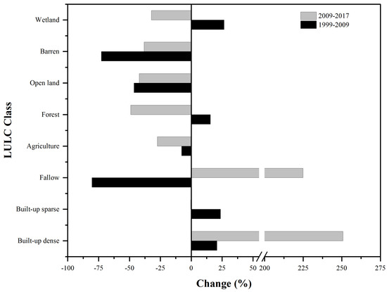
Figure 5.
LULC changes in different classes for the city area (CA) in T1 and T2.
Unoccupied LULC classes, such as open and barren land, record a reduction in both periods, indicating that the increased land consumption by the built-up class takes place at their expense. Open land decreased by 46.3% (T1) and 42.1% (T2) whereas barren land decreased by 72.8% (T1) and 38.2% (T2). With respect to CA another important class is wetland, which increased by 26.6% in T1 followed by a decrease of 32.2% in T2, mostly resulting from climatic and seasonal variations.
3.2. Analysis of Spatial Urbanization Processes
3.2.1. Quantification of Expansion Rate and Intensity
Uer and Uei values were computed at the ward level to measure the spatiotemporal variation observed in the conversion rate and intensity of non-built up to built-up areas in T1 and T2 annually. Overall, in 69 wards of the city Uer is observed to be higher in T2 with an average value of 2.8% as compared to 2.2% in T1. Different wards of the city have considerable variation in the Uer, ranging from 0% to 14% in T1 and 0 to 11.1% in T2. In T1, the highest Uer is observed in most of the wards situated along the fringes. Notably, the highest Uer is found in the wards Khonmoh (14%), Pantha Chowk (8.9%) (south-eastern fringe), Bemina West (8.1%) and Lawaypora (7.5%) (western fringe), Alasteng (7.4%) (northern fringe) (Figure 6).

Figure 6.
Changes in Uer—T1 and T2 categorized according to various classes.
However, the wards located in the centre of the city experienced least to low Uer. In T2, Uer increased as compared to T1, and the highest rates are found in northern fringe wards, namely, Zakora (11.1%), Ahmad Nagar (10.5%), Alasteng (8.6%) and Palapora (8.5%). Central wards, forming the urban core of the city, show minimal addition of built-up land and point towards urban expansion away from the core. In comparison to T1, the city also shows increased Uer around to the core. Increased urban expansion in wards near Dal lake and the northern edge of the river Jhelum is also noticeable. Figure 7a shows the changes in the category of quantified Uer between T1 and T2.

Figure 7.
Changes in category (number of wards (absolute numbers)) of (a) Uer and (b) Uei for T1 and T2.
Conversion of non-built up to built-up land as compared to the available non-built up land in each ward annually is measured through Uei, which reveals a very intensive urbanization pattern in the city. Uei is observed to be more intense in T2 (1%) as compared to T1 (0.6%). In T1, conversion intensity is found to be highest around the fringes on the northern, south-eastern extent and outer limits of the core city (Figure 8). This highlights both the availability of land as well as a preference to develop areas into built-up land away from the city core. The least intensive wards are located around Dal lake, acting as a buffer to urban expansion in other parts of the city. In T2, all wards of the city experienced rapid urbanization. Figure 8 also highlights the increased intensity around northern, north-western and western wards. Similarly, wards encircling the city core also experience rapid conversion of non-built up land. Unlike in T1, wards around Dal lake also come under the ‘High’ and ‘Very High’ categories. Thus, urban expansion pressure extends closer to the wetland in T2 with possible implications for the ecosystem and its services. Category-wise analysis of the Uei, reveals that the number of wards in the ‘Very high’ category increased from a mere 5 in T1 to 16 in T2 i.e., >1.5% increase (Figure 7b), while the number of wards in the ‘Least’ category decreased from 19 in T1 to 10 in T2.

Figure 8.
Changes in Uei—T1 and T2 categorized according to various classes.
3.2.2. Spatiotemporal Trends in Landscape Metrics
The spatial variations in selected landscape metrics at three points in time were analysed to understand the effect of urban growth on landscape pattern such as irregularity, heterogeneity, aggregation and composition. Inner differentiation at city level (which depends on the size and spread of the city) was considered as a benchmark for selecting appropriate cell size. We observed that the selected cell sizes of 2000 2000 m and 1000 1000 m (see supplementary Figures S1 and S2) are non-specific and mismatched to the scale of urban growth in the region. At such coarse cell-size the urban area appears generalized and homogeneous. However, 500 500 m cell size provided more clarity and helped in identifying differentiation at city level while also capturing areas undergoing changes, such as urban fringes and upcoming urban centres in the region. Figure 9, Figure 10, Figure 11 and Figure 12 show the variation of landscape metrics using the resulting thematic maps at 500 m cell size. LPI, denoting the dominance of urban patch as compared to the selected cell area, occupies a smaller and discontinuous area in the centre of Srinagar city in 1999 (Figure 9). In comparison, the years 2009 and 2017 show an expansion of LPI in all directions from city centre, especially in the north, leading to the integration of distant urban areas with the urban core. LSI variation reveals increased irregularity in the shape of built-up areas away from the city core. In 1999, we found the highest LSI mainly in southern and western parts of the city. Outside the city limits, the highest LSI is observed in north-western and south-eastern parts. Our observation indicates early signs of disaggregated growth away from the city. In 2009 and 2017, the highest irregularity in shape is concentrated in southern and south-eastern parts of the city, including regions outside the boundary (Figure 10). Our analysis of LSI also highlights that in many areas within the city limits, increased LSI is succeeded by regions of high LPI value in the following study year. AWMPFD indicates the complexity of the built-up area by considering the perimeter-area ratio. Higher values are found to be more randomly distributed in 1999 as compared to the following years. With continuous urban growth, the city region shows higher patch shape complexity over time and thus increased fragmentation. But in 2009 and 2007, AWMPFD values increased radially away from the city centre specifying areas of the city where built-up area increased in a haphazard manner as the urban core becomes saturated (Figure 11). In comparison to the city, primarily agricultural land in the south and south-eastern region outside the city also shows increased complexity over the years, although less than in the city. AI is an important metrics determining the frequency with which the adjacent matrix of the same class appears side by side. The patterns reveal that built-up areas aggregated predominantly in the city region, with a major increase in the western and northern parts, leading to a larger continuous urban area in 2017. Outside the city boundary, AI is randomly distributed and indicates fragmented growth of urban settlements (Figure 12).

Figure 9.
Largest patch index (LPI) change at 500 m cell-size with enlarged view of CA, year 1999, 2009 and 2017 in the study area.

Figure 10.
Landscape shape index (LSI) change at 500 m cell size with enlarged view of CA, year 1999, 2009 and 2017 in the study area.
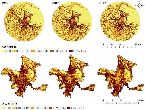
Figure 11.
Area-weighted mean patch fractal dimension (AWMPFD) change at 500 m cell size with enlarged view of CA, year 1999, 2009 and 2017 in the study area.

Figure 12.
Aggregation Index (AI) change at 500 m cell size with enlarged view of CA, year 1999, 2009 and 2017 in the study area.
Other commonly used single-value landscape metrics allow easy comparison to other studies that lack details on spatial variations. NP is found to be the highest (12,628) in 1999, after which it decreases in 2009 (9883) and 2017 (9868). ENNMN shows the lowest value in 2017 (100.83) as compared to 2009 (103.33) and 1999 (103.58), highlighting the reduced edge-to-edge distance between the nearest urban patches. PD is highest in 1999 (6.69) as compared to 2009 (5.24) and 2017 (5.23).
3.2.3. Cluster Analysis of Landscape Structure
To identify the areas that underwent the most significant changes of landscape metrics, spatio-autocorrelation was employed at a cell size of 500 m. Supplementary Figures S3 and S4 highlight the generalized patterns of spatial clustering at 2000 m and 1000 m and affirm the non-suitability of these scales to capture the changes in landscape metrics. Figures S3 and S4 prove no added value of such aggregated spatial scales for urban planning. This is also established by the lack of any significant LSI clusters and inability to identify smaller clusters in other metrics at both scales. Figure 13 illustrates the maps of LISA highlighting the spatial clusters of landscape metrics at 500 m scale along with values of global Moran’s I coefficients.

Figure 13.
Spatial clusters of landscape metrics at 500 m cell-size in 1999, 2009 and 2017 identified through local indicators of spatial association (LISA) along with their global Moran’s I value.
A strong spatial dependence of landscape patterns is visible in terms of values greater than 0.40 of global Moran’s I coefficients. Hotspots of landscape metrics are clearly identifiable through LISA. This result shows clustering in regions with similar landscape metrics values as the adjacent cell. This similarity in the values demonstrate the footprint of the anthropogenic development in the landscape as a result of expansion of the built-up area. Hotspots of LSI and AWMPFD appear in regions further away from the urban core, especially in the north and in isolated areas of the south and south-west of the city. Apart from the urban core, LPI and AI hotspots spread out across the region indicate the development of smaller urban sub-centers, which are utilizing local conditions for an easier expansion into the agricultural region. They could be signs of early urban sprawl. Figure 13 shows the spatial pattern of landscape metrics clustering as a result of similar values in adjacent cells for each year. In contrast, Figure 14 shows the clustering of cells where values of landscape metrics changed most significantly in adjacent cells between two points in time, for example from low value to high value represented by high-high clusters. In CA, other landscape metrics (except LPI) have a clustering of high-high values in a given year (Figure 13) but do not show a drastic increase between years (Figure 14) as compared to areas in OZ. High-high mapped areas, mostly in the OZ (primarily peri-urban areas), experience increased heterogeneity, for example, due to the relative increase in their shape complexity from a low value to a high value. However, changes in LPI are specifically bound to CA as the largest patch is in the city, and most significant changes are only possible in and around it. Between T1 and T2, LPI has shifted from south-east to the northern part of the city. This analytical step indicates the development of fragmented growth outside the CA and is an early sign of urban sprawl. But, low global Moran’s I values indicate such clustering can be a result of random spatial processes.
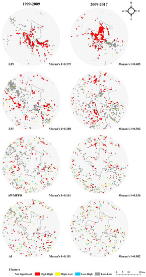
Figure 14.
Spatial clusters of landscape metrics changes at 500 m cell-size between 1999–2009 and 2009–2017 identified through LISA along with their global Moran’s I value.
3.2.4. Spatiotemporal Distribution of Growth Types
Figure 15 shows the distribution of different growth types, primarily depicting the dominance of the edge-expansion type in both T1 and T2. In T1, the proportion of edge-expansion type in the study area (OZ + CA) was 65.8% of the total increase in built-up area, followed by outlying (22.7%) and infilling (11.4%) type growth. As a dominant growth type, edge-expansion is scattered throughout the study area, adding to the previously existing patches mainly in OZ. More prominently, CA shows expansion around old urban patches (defined as the existing built-up area in the previous year) on western and south-eastern fringes of the city. The area adjoining transportation networks links the city with regions outside the administrative boundary and is also characterized by this growth type. The outlying type of growth is mainly found outside the CA, predominantly on the western side, showing signs of urban expansion into agricultural fields. However, the percentage of growth type within CA shows a shift in trend with respect to infilling and outlying growth types. Infilling is observed to be more dominant within CA i.e., 21.4% as compared to 11.6% of outlying, while edge-expansion (67%) remains the dominant growth type. The densification of the urban core by way of infilling is observed mainly on the western edge of the pre-existing urban core, where more housing colonies are constructed and have become densified. The presence of Dal lake on the eastern side has prompted this growth on the western edge, as the initial urban core is densified and unable to accommodate any additional build-up area.
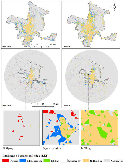
Figure 15.
Spatiotemporal distribution of growth types in T1 (1999–2009) and T2 (2009–2017).
In T2, edge-expansion (65%) remained the dominant growth type followed by outlying (19.2%) and infilling (15.80%) (OZ + CA). However, CA shows a decreasing trend of edge-expansion type (59.7%) while infilling type increased (29.7%). This indicates a densification of existing patches, i.e., the development of unoccupied land within the built-up area while the entire city region continues to grow outwards, connected to existing urban patches. Spatial association can be observed between edge-expansion and infilling types, with infilling dominating (in T2) around the region occupied by edge-expansion (in T1). Major areas experiencing infilling growth are concentrated around the northern extent of the city and the periphery of the urban core. In contrast, the outlying growth type (10.6%) remained a small proportion of overall growth, mainly scattered around northern fringes of the city dominated by agricultural land. Over the two time periods illustrated above, the infilling type is observed to increase within the CA. This growth type is observed to be concentrated in and around the urban core in T1, while in T2 it is dispersed outside the core area. This result indicates the saturation of the urban core and a tendency to densify new areas. Diachronic analysis indicates that the edge-expansion type plays a major role in the expansion of the city outside the urban core.
4. Discussion
4.1. Spatiotemporal Evolution of the Urban Landscape
This study offers a detailed account of urbanization in the largest urban settlement in the Himalaya, providing a gauge to compare urban growth in cities located across different mountain valleys. Evidence from Himalaya suggest an increasing urbanization extent [38,54] along with potential landscape ecological risk from the coupled effects of growth [53]. A major attempt at understanding the urban growth in Himalayan cities was made by Diksha and Kumar [54], analysing their urban sprawl and land consumption pattern. All the capital cities in Himalaya, namely, Srinagar (India), Dehradun (India), Shimla (India), Kathmandu (Nepal), Gangtok (India), Thimpu (Bhutan) and Itanagar (India) were reported to exhibit different growing patterns in terms of densification and dispersion, also highlighting the unplanned and haphazard nature of growth across all mountain and valley cities. One of the similar sized cities in Himalaya is Kathmandu, capital of Nepal, which also reported a complex urbanization pattern comprising scattered growth in some urban areas and densification in others [55], determined through the spatial metrics analysis of this city (increased LPI and decreased ENNMN). However, a lack of detailed studies of urban landscape characteristics in India, and more specifically in other Himalayan cities, forms a major barrier in assessing and comparing these patterns. Further analysis is limited in most studies, as they only provide single landscape metric values for the city, and spatial differentiation is not available. As compared to the other capital cities in Himalaya, Srinagar is observed to have the highest land consumption rate (from 1991–2015) but dispersed growth with less density [54]. Our results also indicate a similar trend of increased rate and intensity in land conversion as well as providing more far-reaching insights by specifying regions experiencing increased irregularity and scattered growth. This was done by providing spatial patterns of landscape metrics and growth type. Other studies on Srinagar have largely provided long-term general patterns of urbanization based on LULC analysis and change detection [38,39,56]. Ward-wise built-up growth points towards significant addition in south and south-eastern wards, validating the increased rate and intensity in the change of the built-up area [56].
However, urban growth in the Srinagar region differs from many of the urban regions in terms of its dominant growth type. Unlike areas assessed in other studies around the world, where the dominant growth type has either differed over time [31,45], including domination by the infilling type of growth [57] or a declining trend in infilling type [45,58], Srinagar (CA and OZ) shows the least contribution of the infilling growth type, although it is increasing gradually, while edge-expansion remained the most dominant type throughout. This indicates a deviating growth trajectory in Himalaya and a need for differential land-use and urban planning strategies not imitated from the non-mountainous regions. Detailed analysis of different measures of urbanization in Srinagar confirms an intensifying growth in and around the urban core while fringes of the city also experience expansion in different directions over time. Our results highlight an increased irregularity and complexity at regional scale, while at city level the urban core experiences an increase in urban patch leading to homogeneity. The city and its surrounding region follow a monocentric urbanization pattern in the absence of any secondary growth points and a continued absorption into the initial urban core. This is also highlighted by an increased LPI in conjunction with an increase in AI values (in 2009 and 2017). Lower values of LSI and AWMPFD values in the urban core indicate a more homogenous pattern of built-up areas. In addition to the densification of the urban core, Srinagar city also experienced a parallel expansion and rapid densification in different parts of the city. However, growth in other parts was marked with increased LSI and AWMPFD, highlighting the increasing irregularity and complexity in patterns of urban growth outward from the urban core.
Considering the urban growth theory proposed by Dietzel et al., (2005) [32] developmental phases of the city are observed to oscillate between two phases, diffusion and coalescence, each following a harmonic pattern [36]. In the case of Srinagar, we could affirm that the city experienced a partial diffusion stage dominated by edge-expansion in T1, while in T2 a decrease in edge-expansion and increase in infilling growth type indicates a transition stage of the ‘wave pattern of urban growth’ which is approaching a coalescence phase. The transition between these stages can also be understood by the gradual changes in other commonly used landscape metrics. In Srinagar, NP is found to be decreasing over the years, indicating an aggregation of urban patches over time. ENNMN shows the lowest value in 2017 as compared to 2009 and 1999, thus highlighting coalescence in later years. High PD in 1999 as compared to 2009 and 2017 also point to the existence of a partial diffusion phase in 1999 followed by coalescence in 2009 and 2017 [37]. However, some studies have reported defined growth phases in selected cities on the basis of single-value landscape metrics [33] or growth types [59]. Anees et al. [33] concluded the existence of well-defined diffusion–aggregation phases in the medium-sized city of Kurukshetra, India. Kantakumar et al. in the study of Pune, India, [59] reported the existence of multiple expansion patterns: coalescence in the urban core and diffusion in the suburbs, that is, a trend towards a polynucleate city. An interesting analysis of 12 Indian cities conducted by Taubenböck et al. [60] derived similarities in the spatial urbanization of different groups of cities, based on landscape metrics among other urbanization indicators. Although all cities belonged to larger population size (>2.5 million), the results from this study point towards a trend wherein a ‘group of cities’ (for example ‘incipient mega cities’ with 5–7 million population) showed signs of urbanization, as was detected in early stages of the next larger group (‘mega cities’ with >10 million population). Similarly, our analysis of Srinagar (1.1 million) is observed to reveal early characteristics of incipient megacities, such as ‘complex urban sprawl in the periphery and densification in the urban core’, but it is still undergoing a transition phase. However, such interpretations should be carefully made, as although aspects of spatial evolution proceed similarly or can be predicted to be similar, detailed analysis of parameters reveal different possible growth patterns. Thus, the growth of Srinagar points toward ill-defined phases which approximate the general ‘diffusion-coalescence’ dichotomy but do not fit it perfectly. Lack of perfect accordance with the theory through deviation from an exact oscillation phase may be due to one of several reported reasons: (i) difference in temporal period, (ii) difference in spatial scale, (iii) possible effects of decade-long conflicts in the Srinagar region from the 1990s. Thus, utilizing landscape metrics along with growth type information, it is possible to understand the growth of the city as a continuum of diffusion and coalescence. This, rather than a dichotomy of these processes, better represents real-world systems [34,48,61].
4.2. Role of Topography, Land-Use Policies, and Recommendations for Spatial Planning
Considering the location of Srinagar on the foothills of the Himalaya, topography plays an important role in shaping the evolution of this city. The presence of mountain chains to the east and south-east of the city has influenced the direction of urban growth. The eastern boundary of the city next to mountains, shows spatially discontinuous growth, with rate and intensity of built-up change ranging mostly from the low to medium category. However, the growth of industrial estates such as Khunmoh (largest industrial area in Srinagar) in the south eastern part of the city, which forms a tail-like structure along the mountains, is an exception to this. The extraction of lime stone for cement production and of quarry stone for the construction of raw material also plays a prominent role in LULC changes along the foothills in this particular area. A general trend of Srinagar’s built-up area expansion to the west coupled with landscape metric values around areas in proximity to the foothills and further constricted by the river Jhelum (in the south-eastern part) points toward increased irregularity and fragmentation. Agricultural land in OZ, west of the foothills, shows a consistent increase in the fragmented built-up area. Thus, topography has put added pressure on specific parts of the urban settlement in the foothills and increased urban expansion into fertile agricultural land in some parts. This phenomenon is also observed through the LISA patterns (Figure 14). They show the most drastic changes in landscape metrics (except LPI) between two points in time being experienced in OZ areas, thus indicating urban sprawl, which changes from simpler shapes to relatively complex shapes between two time points in time.
Weaker policy implementation to protect agricultural land, affordable land prices and greater value returns from urban land along with specific geographic locations are all factors that have traditionally encouraged expansion of the urban footprint into rural agrarian land. The Jammu and Kashmir ‘Land Revenue Act, 1939’ and ‘Agrarian Reforms Act, 1976’ restrict the conversion of agricultural land, but allow land of up to 2 Kanals (0.0005 km2) to be converted without permission, except for some specific crops. As of 2016, lack of a housing policy for rural areas outside the city region has prompted authorities to rely on recommendations from local authorities on a case-by-case manner. LULC results revealed a decrease of 27.5% in agricultural land during T2, up from 7.8% in T1, while the spatial distribution of AI (Figure 12) indicates the aggregation of urban regions in areas previously dominated by agriculture. Special provisions controlling the utilization of non-urbanized land are required which consider the agrarian value of the landscape along with the nature of growth type in the nearby area. The acceleration of urban growth on the north-eastern extent of the city is mostly concentrated around the Srinagar–Leh highway, where expansion was dominated by edge-expansion and infilling growth. The strengthening of the ‘Prevention of Ribbon Development Act, 2007’, which regulates the construction of buildings alongside public roads, is of utmost importance in containing the budding sprawl pattern. A review of the ‘Master Plan 2000–2021’ also shows growth in the north-eastern extents and underdevelopment of the proposed areas in the north-west and south-east of the city due to ineffective land-use policy. This expansion is further constricted by the presence of two wetlands, Dal (on the eastern side) and Anchar (on the western side). However, water bodies are also known to attract human settlements in view of their ecosystem services [62].
To strengthen urban planning measures in India, local municipal bodies which are the closest structures of government to citizens have been granted special provisions in an attempt to decentralize urban governance and provide greater autonomy through the 74th Constitutional Amendment Act. Under this Act, urban local bodies hold the primary responsibility for urban planning and assuring short-term and long-term infrastructural services to citizens. However, many of the cities in India grapple with implementing urban planning measures in a timely and resource-efficient way [23,59,63]. Our results contribute in this regard by providing important information for implementing planning regulation through different proxy measures of urbanization, such as rate, intensity, landscape structure and growth type of the built-up change. In our study, the availability of numerical indices provides a simpler and quantifiable decision-making process, saving valuable time and resources when testing different planning scenarios. As one of the basic steps, municipal bodies should utilize the ward-level data on built-up change rate and intensity to identify specific wards that are facing the highest urbanization pressure. An evaluation of the quality of public services in these wards should be carried out to identify the gaps and to design relevant measures in tune with the LULC information. This can provide a readily comprehensible spatial viewpoint to planning efforts. Based on such information, decision making on resources like roads, water connections, and availability of open, green and blue spaces can be streamlined and incorporated into the long-term plans of the ward. At the city level, management plans should be revised to incorporate a detailed study for the urban landscape structure, including spatial differentiation of landscape metrics in the city. Such spatial information should be utilized to identify the area experiencing irregular and fragmented urban growth. Analysing areas that show such temporally consistent trends would be helpful in enforcing building by-laws and the provisions of the master plan, which restricts haphazard growth within the city limits, especially in the urban fringes. Information from landscape metrics like LPI and AI should be utilized to understand the densification trend of the city and to achieve a sustainable balance between compaction and sprawl. Thus, quantitative measures of the complex landscapes can serve as criteria for assisting the decision-making process [60,64]. At a regional level, we recommend synchronizing the type of infrastructural development with the identified growth phase of the city, which also affects the rural characteristics in the region. Prior knowledge of the growth phase, such as coalescence, should be used to develop a transport infrastructure which supports infill development and promotes densification. Various types of roads have a major role in influencing urban landscape composition and configuration [25]. At the same time, limiting the conversion of open land to built-up during the coalescence phase can allow the development of green spaces, providing valuable ecosystem services. Promoting infilling development in the urban areas experiencing edge-expansion and outlying growth, symbolizing the diffusion phase, would help in conserving resources and reduce land fragmentation, thus preserving more ecologically valuable lands. A combination of landscape metrics and various growth types can be used to identify agricultural land around the city that is most vulnerable to land conversion. Furthermore, to strengthen spatial planning initiatives, spatio-autocorrelation must be employed to identify hotspots of change, as they provide direct interpretable results from landscape metrics.
4.3. Methodological Improvements and Limitations
Within urban regions, intra-level landscape diversity and local differences can also contribute to spatial planning and management [65]. The majority of the studies analysing landscape structure focus on a single-value metric for the city and utilize it for interpretations of landscape characteristics and/or phases of urban growth. In this study, one of the key innovative methodologies used is spatial differentiation of landscape metrics, which is achieved by using grids of different sizes. For this, identification of appropriate cell size is critical, as urban regions undergo rapid change compared to other land-use forms and are thus expected to create greater localized differences in the landscape. Other regional studies involving a larger urban region with multiple cities [18,25] have adopted 5 km and 10 km as the scale of analysis for landscape metrics. By testing intermediate cell sizes of 500 m, 1000 m and 2000 m, we were able to identify the appropriate scale, i.e., 500 m, capable of reflecting diversity in composition and configuration in a region sized approximately 2000 km2. However, the accuracy of the results is limited by the medium resolution of remote-sensing data and can be further improved by utilizing high-resolution data. Uncertainty and errors are also expected from various algorithms of image classification, so that future research can fruitfully explore the possibility of testing multiple algorithms and classification techniques. Considering a broader time scale for analysis will also provide clearer trends of urban growth over time. As temporally limited studies are less efficient in observing the exact oscillating urban growth pattern, a wider temporal scale analysis of urban dynamics would bring more clarity to the growth phase debate.
5. Conclusions
An integrated multi-scale approach utilizing remote-sensing and GIS tools was implemented in this study to gain a spatially explicit understanding of urban dynamics in and around Srinagar city from 1999 to 2017. Globally, many studies have contributed to our understanding of spatiotemporal patterns of urban growth. However, spatial differences within computed landscape metrics are rarely addressed, and thus their contribution in urban planning is limited. In this study, we utilized satellite data to delineate (i) measures indicating urban growth of the city and its environs, (ii) urban growth patterns and processes at different spatiotemporal scales and (iii) the typology of urban growth in different parts of the city. Based on our results and their analysis, we conclude the following:
- Srinagar has experienced considerable urban growth at the expense of fertile agricultural land, forest and open land. In the absence of any major urban centre nearby, Srinagar city has accommodated most of the growth in the region, while outside the city boundary expansion was observed mainly in the south and south-eastern region. Within the city, the rate and intensity of different built-up areas in wards highlight spatial variation in two time periods. Identification of specific wards undergoing rapid changes in the city is an important step towards implementing urban planning measures and resolving the reduction in open and green spaces.
- The analysis of landscape metrics based on spatial differentiation helps in deducing the inner urban structural pattern of the city. At the selected 500 m cell size, areas were identified experiencing irregular, fragmented and compact growth. An integrated approach to quantifying urban expansion by means of landscape metrics and further identification of hotspots using spatial autocorrelation is highly efficient and feasible, providing scientific criteria to prioritize areas that require appropriate policy implementation.
- In terms of urban growth typology, Srinagar city is dominated by the edge-expansion growth type, then followed by the infilling and outlying types. In association with landscape metrics results, the urban development trajectory of Srinagar points towards a mixed phase of different growth processes. Over the span of almost three decades, the city experienced a domination of diffusion in the initial year of investigation, followed by the dominance of a coalescence phase. Increased irregularity and fragmentation beyond the urban core, and increased aggregation and homogeneity within the core highlight the continuum of diffusion-coalescence even within the prevalent phase mentioned.
Supplementary Materials
The following are available online at https://www.mdpi.com/2072-4292/12/8/1306/s1, Figure S1: Landscape metrics (LPI, LSI, AWMPFD and AI) change at 2000 m cell size- year 1999, 2009 and 2017, Figure S2: Landscape metrics (LPI, LSI, AWMPFD and AI) change at 1000 m cell size- year 1999, 2009 and 2017, Figure S3: Spatial clusters of landscape metrics at 2000 m cell-size in 1999, 2009 and 2017 identified through LISA along with their Global Moran’s I value, Figure S4: Spatial clusters of landscape metrics at 1000 m cell-size in 1999, 2009 and 2017 identified through LISA along with their Global Moran’s I value, Table S1: Administrative wards of Srinagar city, Table S2: Details of satellite data used, Table S3: Characterisation of LULC classes, Table S4: Number of reference sites associated with each class generated by probability proportional to size (PPS) sampling technique.
Author Contributions
Conceptualization, M.M.A. and P.K.J.; Methodology, M.M.A., D.M. and P.K.J.; Software, D.M. and M.S.; Validation, D.M., M.S., E.B. and P.K.J.; Formal Analysis, M.M.A. and D.M.; Investigation, M.M.A. and D.M.; Resources, E.B. and P.K.J.; Data Curation, M.M.A. and M.S.; Writing-Original Draft Preparation, M.M.A.; Writing-Review & Editing, E.B. and P.K.J.; Visualization, M.M.A. and D.M.; Supervision, P.K.J. and E.B. All authors have read and agreed to the published version of the manuscript.
Funding
This research received no external funding and The APC was funded by Helmholtz Centre for Environmental Research.
Acknowledgments
M.M.A. would like to express his gratitude for the research support from University Grants Commission (UGC) for Senior Research Fellowship (SRF) and DAAD (Deutscher Akademischer Austauschdienst). D.M. acknowledges DAAD support. P.K.J. is thankful to Department of Science and Technology—Promotion of University Research and Scientific Excellence (DST-PURSE) of Jawaharlal Nehru University (JNU), New Delhi for research support.
Conflicts of Interest
The authors declare no conflict of interest. The funders had no role in the design of the study; in the collection, analyses, or interpretation of data; in the writing of the manuscript, or in the decision to publish the results.
References
- McDonnell, M.J.; Pickett, S.T.A. Ecosystem Structure and Function along Urban-Rural Gradients: An Unexploited Opportunity for Ecology. Ecology 1990, 71, 1232–1237. [Google Scholar] [CrossRef]
- Pickett, S.T.A.; Cadenasso, M.L.; Grove, J.M.; Boone, C.G.; Groffman, P.M.; Irwin, E.; Kaushal, S.S.; Marshall, E.; McGrath, B.P.; Nilon, C.H.; et al. Urban ecological systems: Scientific foundations and a decade of progress. J. Environ. Manage. 2011, 92, 331–362. [Google Scholar] [CrossRef] [PubMed]
- Banzhaf, E.; Kabisch, S.; Knapp, S.; Rink, D.; Wolff, M.; Kindler, A. Integrated research on land-use changes in the face of urban transformations—An analytic framework for further studies. Land Use Policy 2017, 60, 403–407. [Google Scholar] [CrossRef]
- Zhang, X.Q. The trends, promises and challenges of urbanisation in the world. Habitat Int. 2016, 54, 241–252. [Google Scholar] [CrossRef]
- Bai, X.; Shi, P.; Liu, Y. Realizing China’s urban dream. Nature 2014, 509, 158–160. [Google Scholar] [CrossRef] [PubMed]
- Swerts, E.; Pumain, D.; Denis, E. The future of India’s urbanization. Futures 2014, 56, 43–52. [Google Scholar] [CrossRef]
- United Nations, Department of Economic and Social Affairs PD. World Urbanization Prospects: The 2018 Revision (ST/ESA/SER.A/420); United Nations: New York, NY, USA, 2019. [Google Scholar]
- Klopp, J.M.; Petretta, D.L. The urban sustainable development goal: Indicators, complexity and the politics of measuring cities. Cities 2017, 63, 92–97. [Google Scholar] [CrossRef]
- Bettencourt, L.M.A. The Origins of Scaling in Cities. Science 2013, 340, 1438–1442. [Google Scholar] [CrossRef]
- McPhearson, T.; Haase, D.; Kabisch, N.; Gren, Å. Advancing understanding of the complex nature of urban systems. Ecol. Indic. 2016, 70, 566–573. [Google Scholar] [CrossRef]
- Lausch, A.; Blaschke, T.; Haase, D.; Herzog, F.; Syrbe, R.U.; Tischendorf, L.; Walz, U. Understanding and quantifying landscape structure—A review on relevant process characteristics, data models and landscape metrics. Ecol. Modell. 2015, 295, 31–41. [Google Scholar] [CrossRef]
- Wang, H.; He, Q.; Liu, X.; Zhuang, Y.; Hong, S. Global urbanization research from 1991 to 2009: A systematic research review. Landsc. Urban Plan. 2012, 104, 299–309. [Google Scholar] [CrossRef]
- Zhu, Z.; Zhou, Y.; Seto, K.C.; Stokes, E.C.; Deng, C.; Pickett, S.T.A.; Taubenbock, H. Understanding an urbanizing planet: Strategic directions for remote sensing. Remote Sens. Environ. 2019, 228, 164–182. [Google Scholar] [CrossRef]
- Seto, K.C.; Sánchez-Rodríguez, R.; Fragkias, M. The New Geography of Contemporary Urbanization and the Environment. Annu. Rev. Environ. Resour. 2010, 35, 167–194. [Google Scholar] [CrossRef]
- Estoque, R.C.; Murayama, Y. Intensity and spatial pattern of urban land changes in the megacities of Southeast Asia. Land Use Policy 2015, 48, 213–222. [Google Scholar] [CrossRef]
- Dadashpoor, H.; Azizi, P.; Moghadasi, M. Land use change, urbanization, and change in landscape pattern in a metropolitan area. Sci. Total Environ. 2019, 655, 707–719. [Google Scholar] [CrossRef] [PubMed]
- Fan, C.; Myint, S. A comparison of spatial autocorrelation indices and landscape metrics in measuring urban landscape fragmentation. Landsc. Urban Plan. 2014, 121, 117–128. [Google Scholar] [CrossRef]
- Su, S.; Jiang, Z.; Zhang, Q.; Zhang, Y. Transformation of agricultural landscapes under rapid urbanization: A threat to sustainability in Hang-Jia-Hu region, China. Appl. Geogr. 2011, 31, 439–449. [Google Scholar] [CrossRef]
- Herold, M.; Couclelis, H.; Clarke, K.C. The role of spatial metrics in the analysis and modeling of urban land use change. Comput. Environ. Urban Syst. 2005, 29, 369–399. [Google Scholar] [CrossRef]
- Herold, M.; Scepan, J.; Clarke, K.C. The use of remote sensing and landscape metrics to describe structures and changes in urban land uses. Environ. Plan. A 2002, 34, 1443–1458. [Google Scholar] [CrossRef]
- Fenta, A.A.; Yasuda, H.; Haregeweyn, N.; Belay, A.S.; Hadush, Z.; Gebremedhin, M.A.; Mekonnen, G. The dynamics of urban expansion and land use/land cover changes using remote sensing and spatial metrics: The case of Mekelle City of northern Ethiopia. Int. J. Remote Sens. 2017, 38, 4107–4129. [Google Scholar] [CrossRef]
- Huang, J.; Lu, X.X.; Sellers, J.M. A global comparative analysis of urban form: Applying spatial metrics and remote sensing. Landsc. Urban Plan. 2007, 82, 184–197. [Google Scholar] [CrossRef]
- Ramachandra, T.V.; Bharath, H.; Durgappa, D. Insights to urban dynamics through landscape spatial pattern analysis. Int. J. Appl. Earth Obs. Geoinf. 2012, 18, 329–343. [Google Scholar] [CrossRef]
- Reis, J.P.; Silva, E.A.; Pinho, P. Spatial metrics to study urban patterns in growing and shrinking cities. Urban Geogr. 2016, 37, 246–271. [Google Scholar] [CrossRef]
- Tan, R.; Liu, Y.; Liu, Y.; He, Q.; Ming, L. Urban growth and its determinants across the Wuhan urban agglomeration, central China. Habitat Int. 2014, 44, 268–281. [Google Scholar] [CrossRef]
- Hu, X.; Xu, H. A new remote sensing index for assessing the spatial heterogeneity in urban ecological quality: A case from Fuzhou City, China. Ecol. Indic. 2018, 89, 11–21. [Google Scholar] [CrossRef]
- Aldwaik, S.Z.; Gilmore, R.J.P. Intensity analysis to unify measurements of size and stationarity of land changes by interval, category, and transition. Landsc. Urban Plan. 2012, 106, 103–114. [Google Scholar] [CrossRef]
- Pili, S.; Serra, P.; Salvati, L. Landscape and the city: Agro-forest systems, land fragmentation and the ecological network in Rome, Italy. Urban For. Urban Green. 2019, 41, 230–237. [Google Scholar] [CrossRef]
- Shi, Y.; Sun, X.; Zhu, X.; Li, Y.; Mei, L. Characterizing growth types and analyzing growth density distribution in response to urban growth patterns in peri-urban areas of Lianyungang City. Landsc. Urban Plan. 2012, 105, 425–433. [Google Scholar] [CrossRef]
- Wilson, E.H.; Hurd, J.D.; Civco, D.L.; Prisloe, M.P.; Arnold, C. Development of a geospatial model to quantify, describe and map urban growth. Remote Sens. Environ. 2003, 86, 275–285. [Google Scholar] [CrossRef]
- Sun, C.; Wu, Z.; Lv, Z.; Yao, N.; Wei, J. Quantifying different types of urban growth and the change dynamic in Guangzhou using multi-temporal remote sensing data. Int. J. Appl. Earth Obs. Geoinf. 2013, 21, 409–417. [Google Scholar] [CrossRef]
- Dietzel, C.; Oguz, H.; Hemphill, J.J.; Clarke, K.C.; Gazulis, N. Diffusion and coalescence of the Houston Metropolitan Area: Evidence supporting a new urban theory. Environ. Plan. B Plan. Des. 2005, 32, 231–246. [Google Scholar] [CrossRef]
- Anees, M.M.; Sajjad, S.; Joshi, P.K. Characterizing urban area dynamics in historic city of Kurukshetra, India, using remote sensing and spatial metric tools. Geocarto Int. 2018, 34, 1–24. [Google Scholar] [CrossRef]
- Dietzel, C.; Herold, M.; Hemphill, J.J.; Clarke, K.C. Spatio-temporal dynamics in California’s Central Valley: Empirical links to urban theory. Int. J. Geogr. Inf. Sci. 2005, 19, 175–195. [Google Scholar] [CrossRef]
- Xu, C.; Liu, M.; Zhang, C.; An, S.; Yu, W.; Chen, J.M. The spatiotemporal dynamics of rapid urban growth in the Nanjing metropolitan region of China. Landsc. Ecol. 2007, 22, 925–937. [Google Scholar] [CrossRef]
- Liu, X.; Li, X.; Chen, Y.; Tan, Z.; Li, S.; Ai, B. A new landscape index for quantifying urban expansion using multi-temporal remotely sensed data. Landsc. Ecol. 2010, 25, 671–682. [Google Scholar] [CrossRef]
- Qu, W.; Zhao, S.; Sun, Y. Spatiotemporal patterns of urbanization over the past three decades: A comparison between two large cities in Southwest China. Urban Ecosyst. 2014, 17, 723–739. [Google Scholar] [CrossRef]
- Nengroo, Z.A.; Bhat, M.S.; Kuchay, N.A. Measuring urban sprawl of Srinagar city, Jammu and Kashmir, India. J. Urban Manag. 2017, 6, 45–55. [Google Scholar] [CrossRef]
- Amin, A.; Fazal, S. Evaluating Urban Landscape Dynamics over Srinagar City and Its Environs. J. Geogr. Inf. Syst. 2015, 7, 211–225. [Google Scholar] [CrossRef]
- Congalton, R.G.; Green, K. Assessing the Accuracy of Remotely Sensed Data-Principles and Practices; Lewis Publishers-CRC Press: Boca Raton, FL, USA, 1999. [Google Scholar]
- Ma, Y.; Xu, R. Remote sensing monitoring and driving force analysis of urban expansion in Guangzhou City, China. Habitat Int. 2010, 34, 228–235. [Google Scholar] [CrossRef]
- Xu, X.; Min, X. Quantifying spatiotemporal patterns of urban expansion in China using remote sensing data. Cities 2013, 35, 104–113. [Google Scholar] [CrossRef]
- Banzhaf, E.; Kindler, A.; Muller, A.; Metz, K.; Reyes-Paecke, S.; Weiland, U. Land-use change, risk and land-use management. In Risk Habitat Megacity; Heinrichs, D., Krellenberg, K., Hansjurgens, B., Martinex, F., Eds.; Springer: Berlin, Germany, 2012. [Google Scholar]
- Tian, G.; Jiang, J.; Yang, Z.; Zhang, Y. The urban growth, size distribution and spatio-temporal dynamic pattern of the Yangtze River Delta megalopolitan region, China. Ecol. Modell. 2011, 222, 865–878. [Google Scholar] [CrossRef]
- Dahal, K.R.; Benner, S.; Lindquist, E. Urban hypotheses and spatiotemporal characterization of urban growth in the Treasure Valley of Idaho, USA. Appl. Geogr. 2017, 79, 11–25. [Google Scholar] [CrossRef]
- Botequilha Leitão, A.; Ahern, J. Applying landscape ecological concepts and metrics in sustainable landscape planning. Landsc. Urban Plan. 2002, 59, 65–93. [Google Scholar] [CrossRef]
- Triantakonstantis, D.; Stathakis, D. Examining urban sprawl in Europe using spatial metrics. Geocarto Int. 2015, 30, 1092–1112. [Google Scholar] [CrossRef]
- Zhao, J.; Zhu, C.; Zhao, S. Comparing the Spatiotemporal Dynamics of Urbanization in Moderately Developed Chinese Cities over the Past Three Decades: Case of Nanjing and Xi’an. J. Urban Plan. Dev. 2015, 141, 1–9. [Google Scholar] [CrossRef]
- McGarigal, K. FRAGSTATS. FRAGSTATS HELP; University of Massachusetts: Amherst, MA, USA, 2015; Available online: https://www.umass.edu/landeco/research/fragstats/documents/fragstats.help.4.2.pdf (accessed on 9 April 2020).
- McGarial, K.; Marks, B. FRAGSTAT: Spatial Pattern Analysis Program for Quantifying Landscape Structure; United States Dep Agric Pacific Northwest Res Station: Portland, OR, USA, 1995; p. 120.
- Forman, R. Land Mosaics: The ecology of Landscapes and Regions; Cambridge University Press: Cambridge, UK, 1995. [Google Scholar]
- Anselin, L. Interactive techniques and exploratory spatial data analysis. In Geographical Information Systems; Longley, P.A., Godchild, M.F., Maguire, D.J., Eds.; John Wiley & Sons: New York, NY, USA, 1999; Volume 37, pp. 291–296. [Google Scholar]
- Mann, D.; Agrawal, G.; Joshi, P.K. Spatio-temporal forest cover dynamics along road networks in the Central Himalaya. Ecol. Eng. 2019, 127, 383–393. [Google Scholar] [CrossRef]
- Diksha, K.A. Analysing urban sprawl and land consumption patterns in major capital cities in the Himalayan region using geoinformatics. Appl. Geogr. 2017, 89, 112–123. [Google Scholar] [CrossRef]
- Thapa, R.B.; Murayama, Y. Examining spatiotemporal urbanization patterns in Kathmandu Valley, Nepal: Remote sensing and spatial metrics approaches. Remote Sens. 2009, 1, 534–556. [Google Scholar] [CrossRef]
- Ahmad, T.; Pandey, A.C.; Kumar, A. Evaluating urban growth and its implication on flood hazard and vulnerability in Srinagar city, Kashmir Valley, using geoinformatics. Arab. J. Geosci. 2019, 1–20. [Google Scholar] [CrossRef]
- Wu, W.; Zhao, S.; Zhu, C.; Jiang, J. A comparative study of urban expansion in Beijing, Tianjin and Shijiazhuang over the past three decades. Landsc. Urban Plan. 2015, 134, 93–106. [Google Scholar] [CrossRef]
- Jiao, L.; Liu, J.; Xu, G.; Dong, T.; Gu, Y.; Zhang, B.; Liu, Y.; Liu, X. Proximity Expansion Index: An improved approach to characterize evolution process of urban expansion. Comput. Environ. Urban Syst. 2018, 70, 102–112. [Google Scholar] [CrossRef]
- Kantakumar, L.N.; Kumar, S.; Schneider, K. Spatiotemporal urban expansion in Pune metropolis, India using remote sensing. Habitat Int. 2016, 51, 11–22. [Google Scholar] [CrossRef]
- Taubenböck, H.; Wegmann, M.; Roth, A.; Mehl, H.; Dech, S. Urbanization in India—Spatiotemporal analysis using remote sensing data. Comput. Environ. Urban Syst. 2009, 33, 179–188. [Google Scholar] [CrossRef]
- Jenerette, G.D.; Potere, D. Global analysis and simulation of land-use change associated with urbanization. Landsc. Ecol. 2010, 25, 657–670. [Google Scholar] [CrossRef]
- Riera, J.; Voss, P.R.; Carpenter, S.R.; Kratz, T.K.; Lillesand, T.M.; Schnaiberg, J.A.; Turner, M.G.; Wegener, M.W. Nature, society and history in two contrasting landscapes in Wisconsin, USA Interactions between lakes and humans during the twentieth century. Land Use Policy. 2001, 18, 41–51. [Google Scholar] [CrossRef]
- Abhishek, N.; Jenamani, M.; Mahanty, B. Urban growth in Indian cities: Are the driving forces really changing? Habitat Int. 2017, 69, 48–57. [Google Scholar] [CrossRef]
- Weng, Y.C. Spatiotemporal changes of landscape pattern in response to urbanization. Landsc. Urban Plan. 2007, 81, 341–353. [Google Scholar] [CrossRef]
- Yeh, C.T.; Huang, S.L. Investigating spatiotemporal patterns of landscape diversity in response to urbanization. Landsc. Urban Plan. 2009, 93, 151–162. [Google Scholar] [CrossRef]


© 2020 by the authors. Licensee MDPI, Basel, Switzerland. This article is an open access article distributed under the terms and conditions of the Creative Commons Attribution (CC BY) license (http://creativecommons.org/licenses/by/4.0/).