Monitoring Effect of Spatial Growth on Land Surface Temperature in Dhaka

 ,
,  ,
,  ,
,  ,
,  ,
,  ,
,  ,
,  ,
,  ,
,  ,
,  and
and 
Abstract

1. Introduction
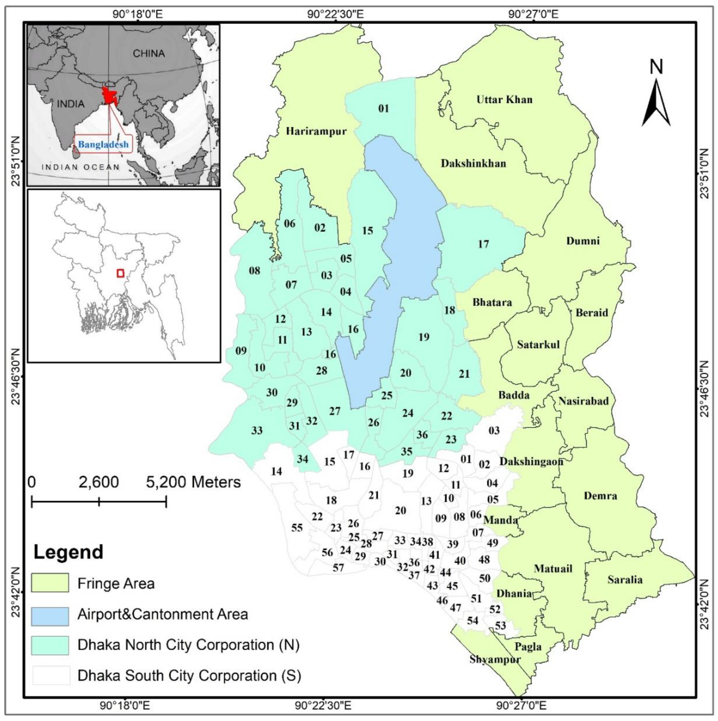
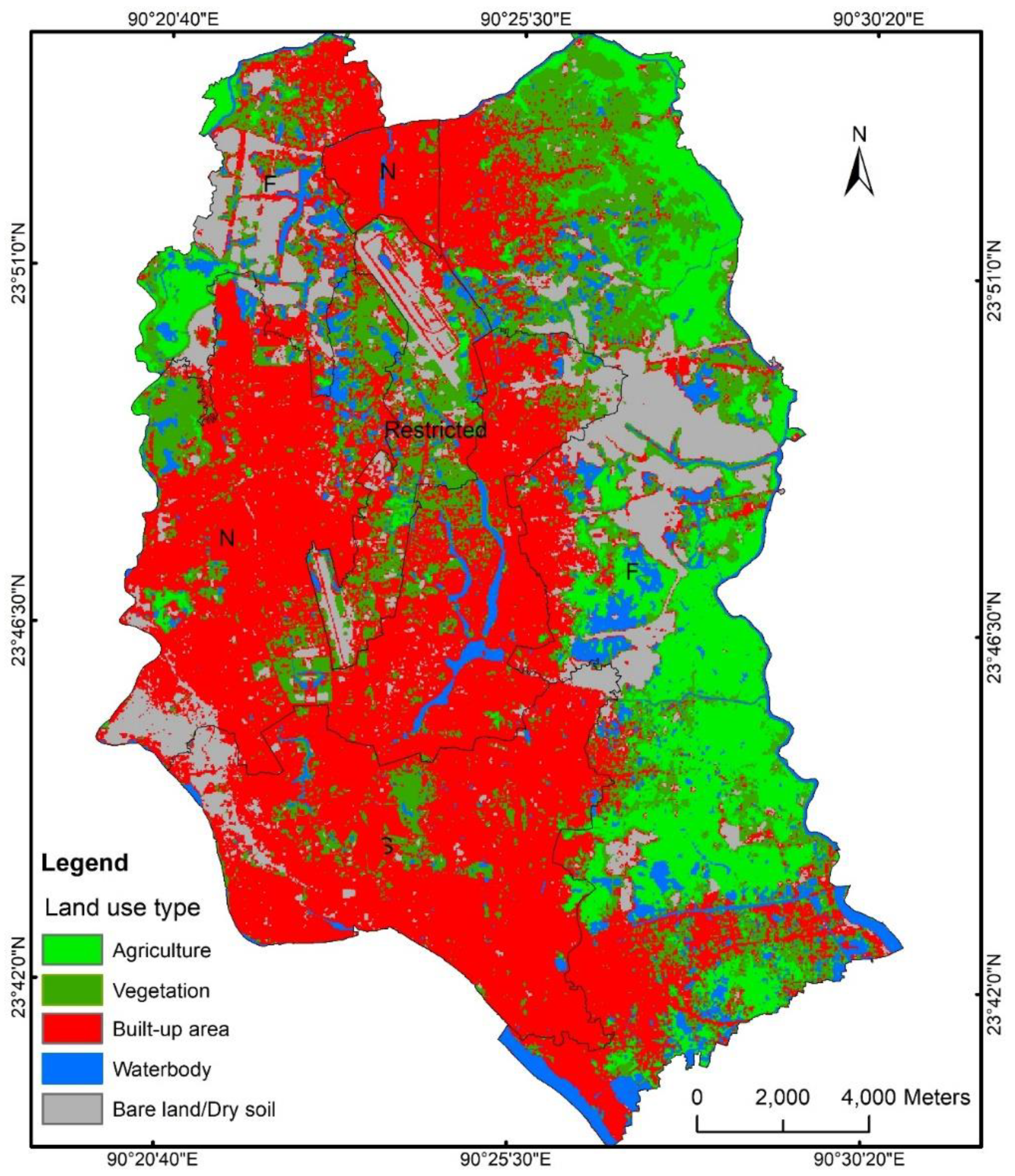
2. Study Area
3. Materials and Methods
3.1. Data Sets
3.1.1. TanDEM-X
3.1.2. ASTER GDEM V2
3.1.3. AW3D30
3.1.4. Landsat-8 OLI/TIRS
3.1.5. Reference Data
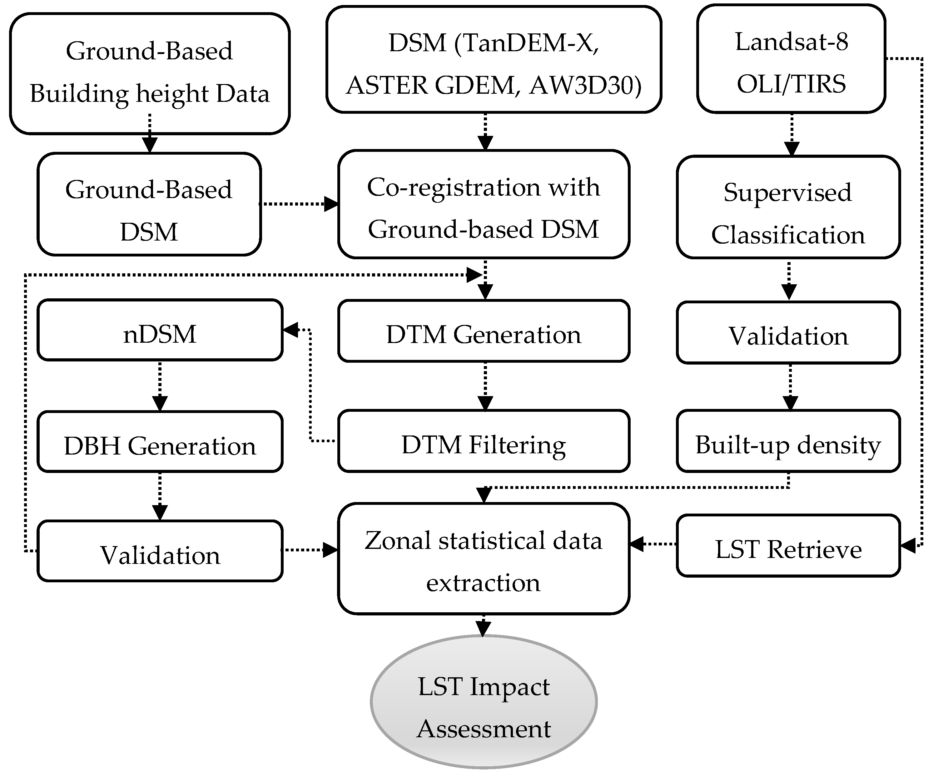
3.2. Method
3.2.1. Vertical Growth Assessment
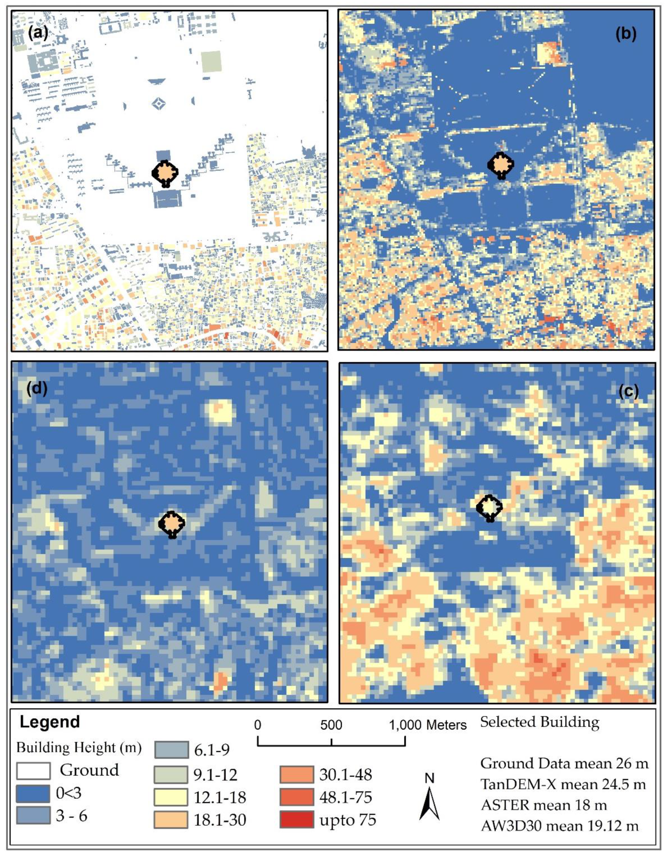
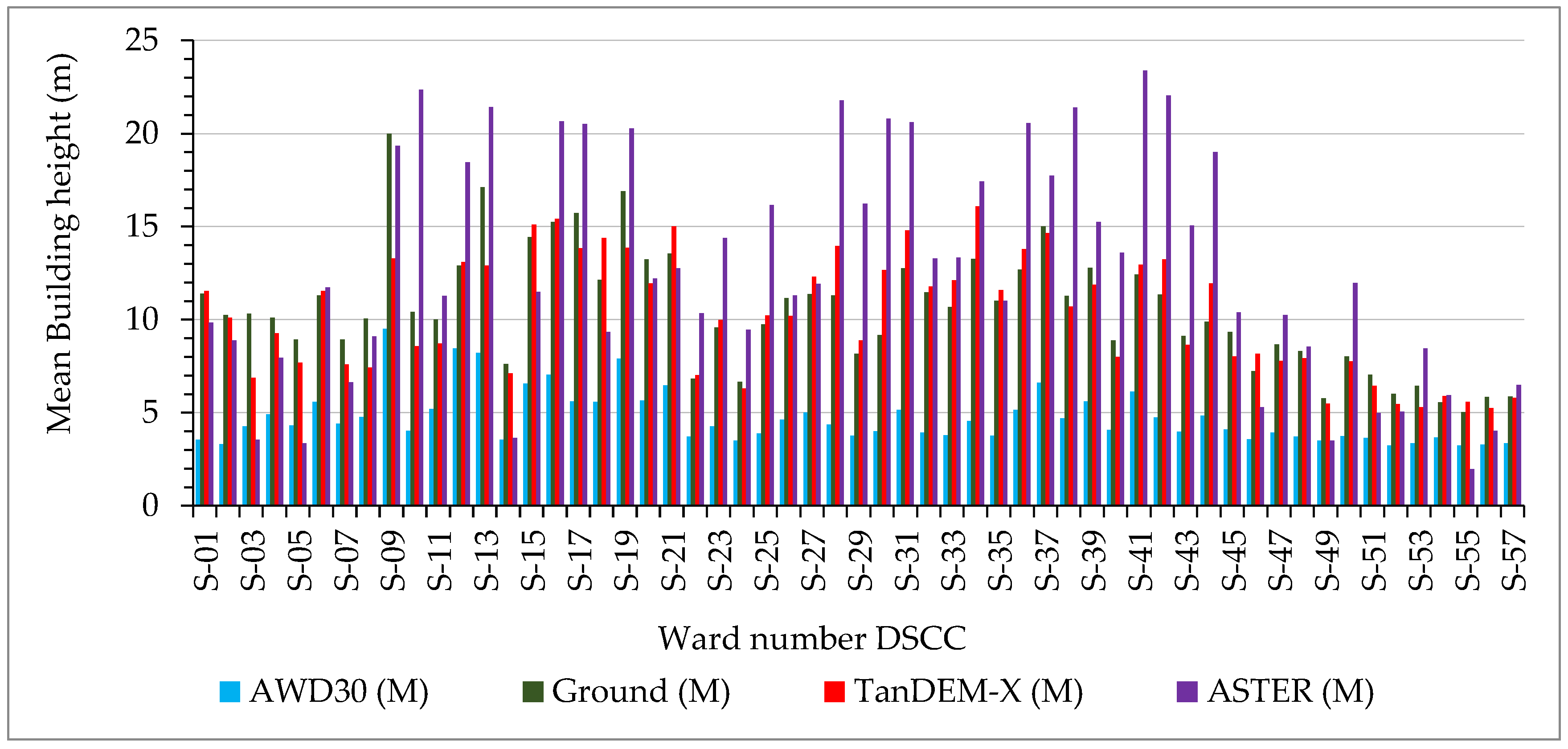
3.2.2. Building Height Extraction
3.2.3. Built-Up Density (BUD) Analysis
3.2.4. Land Surface Temperature (LST) Retrieval
3.2.5. LST Impact Assessment
4. Results
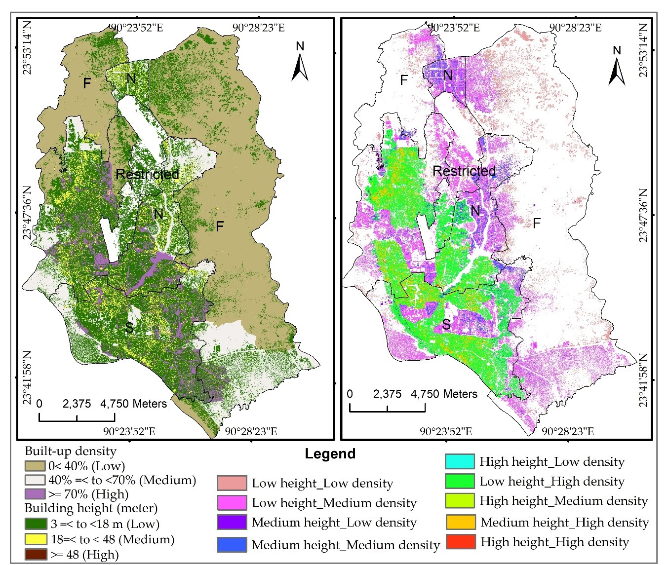
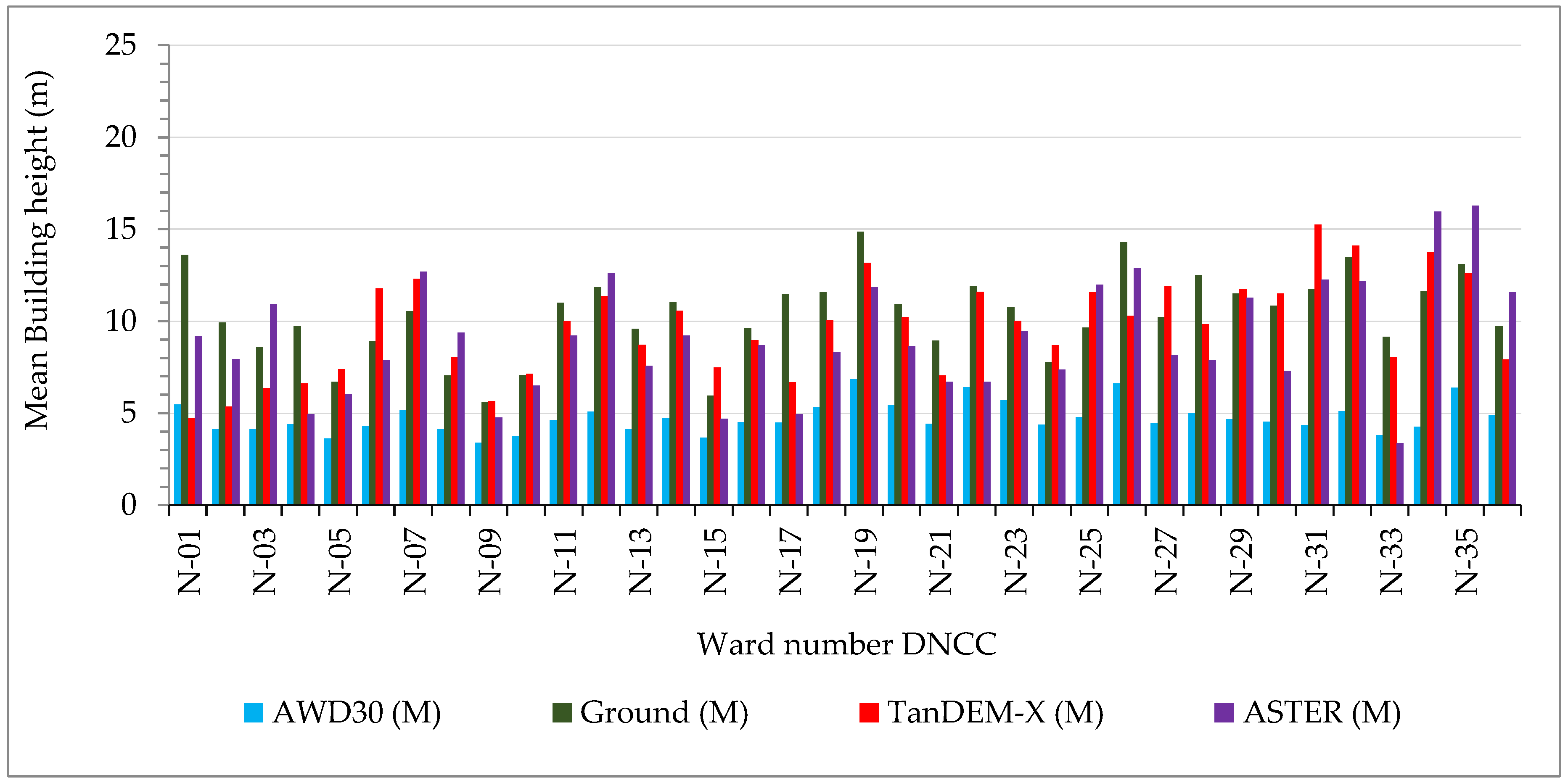
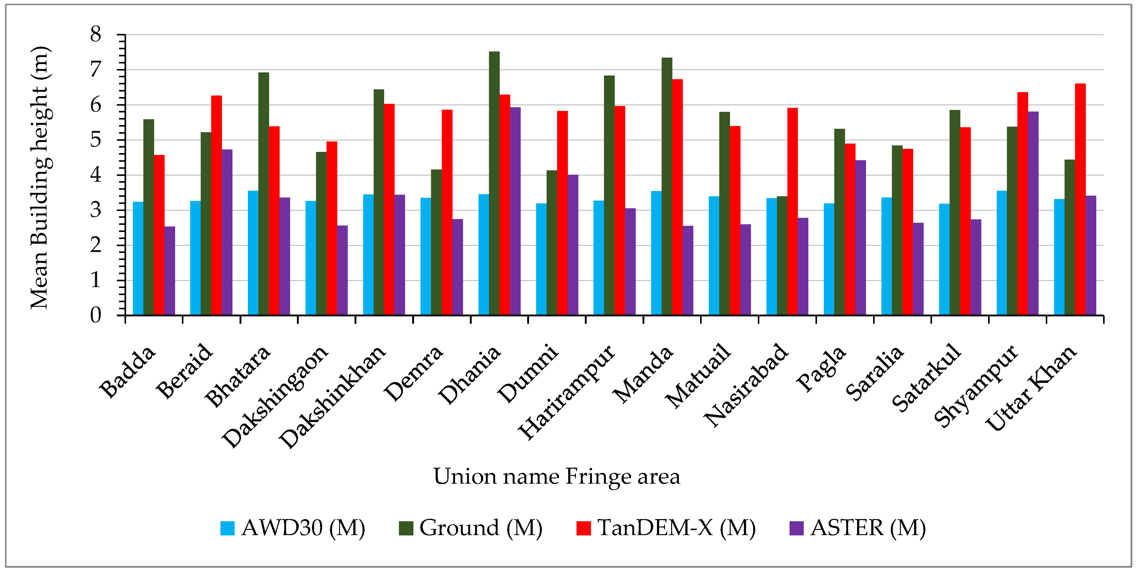
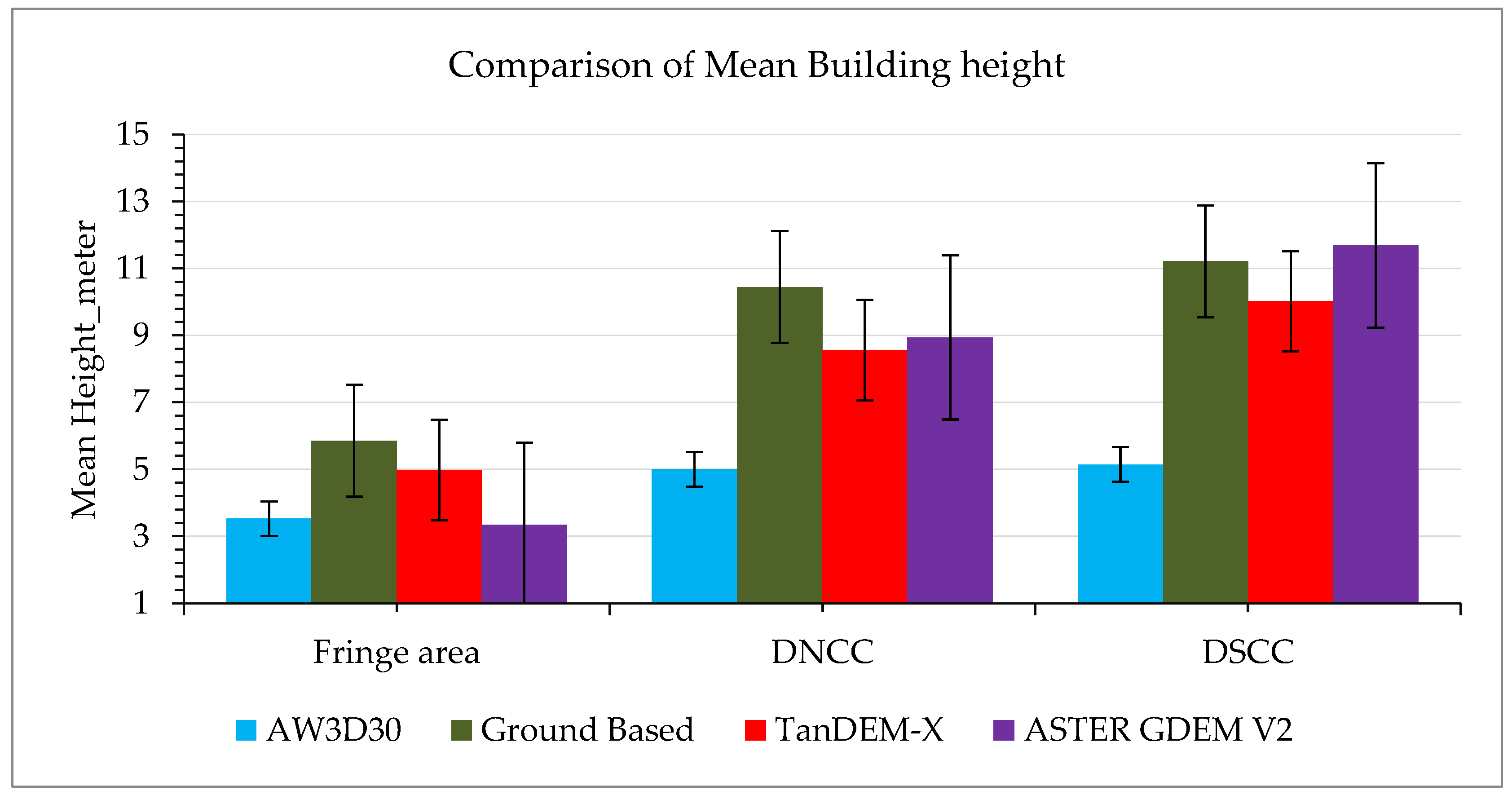
4.1. Building Height
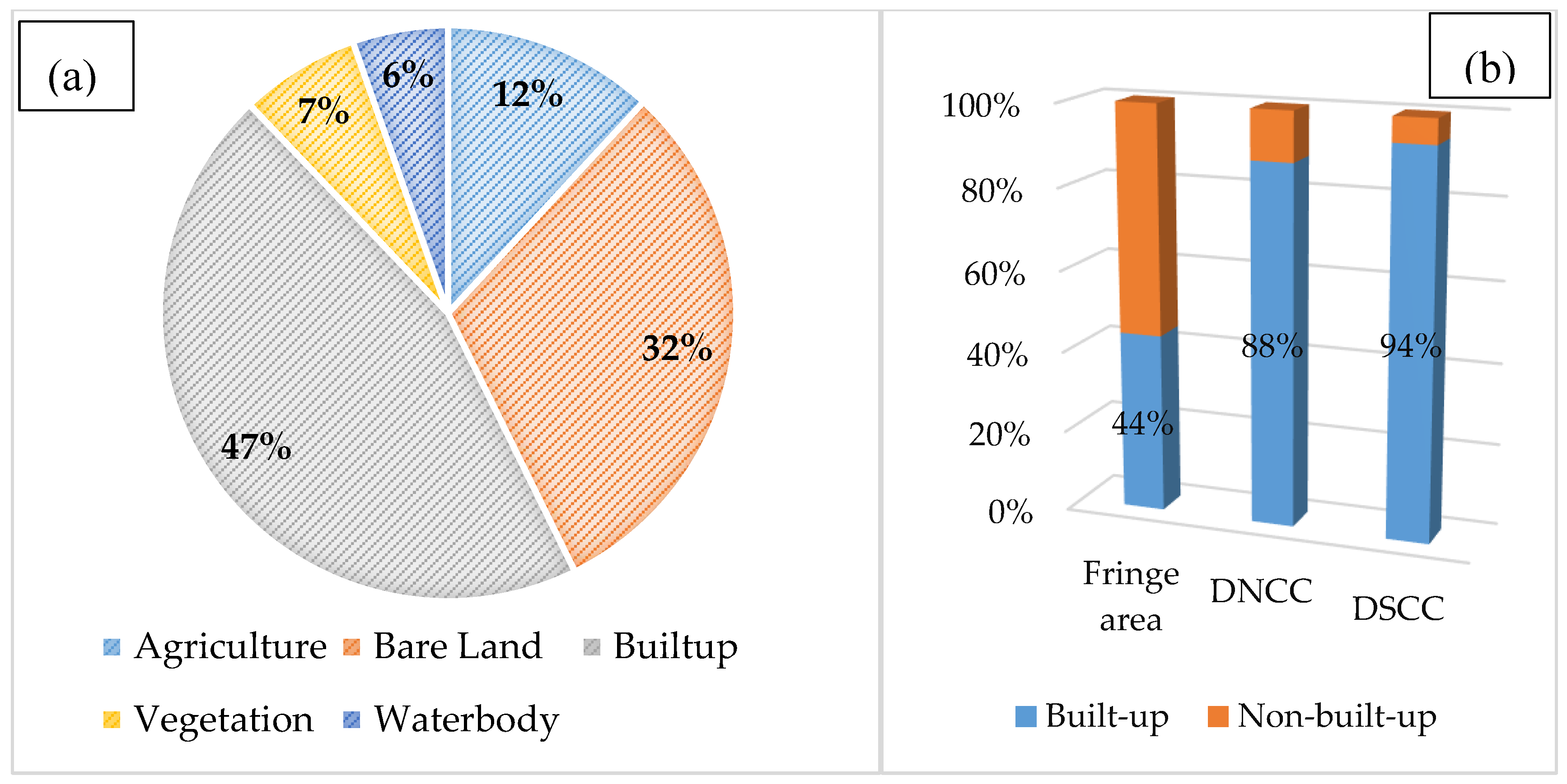
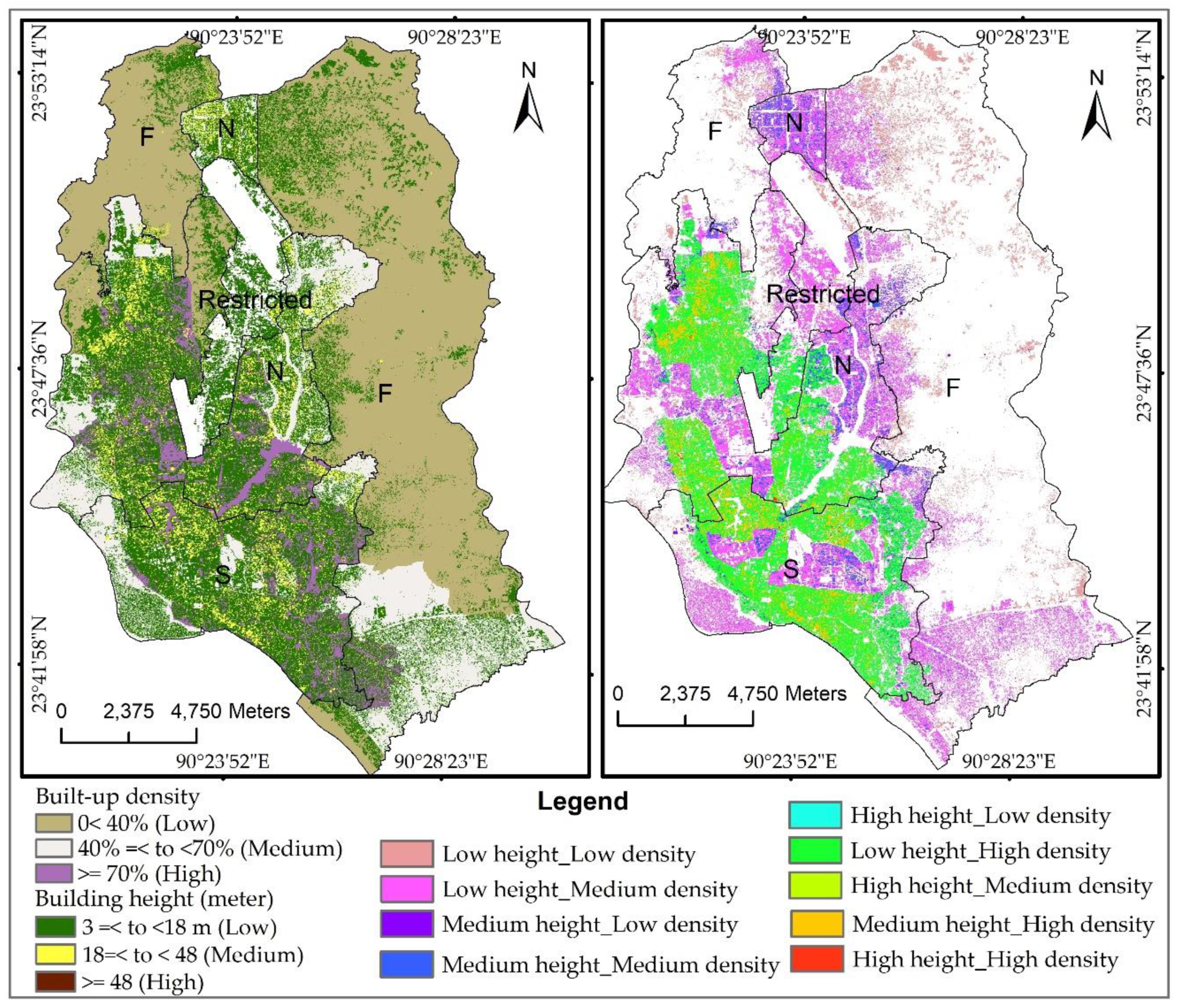
4.2. Built-Up Density and Landscape Pattern
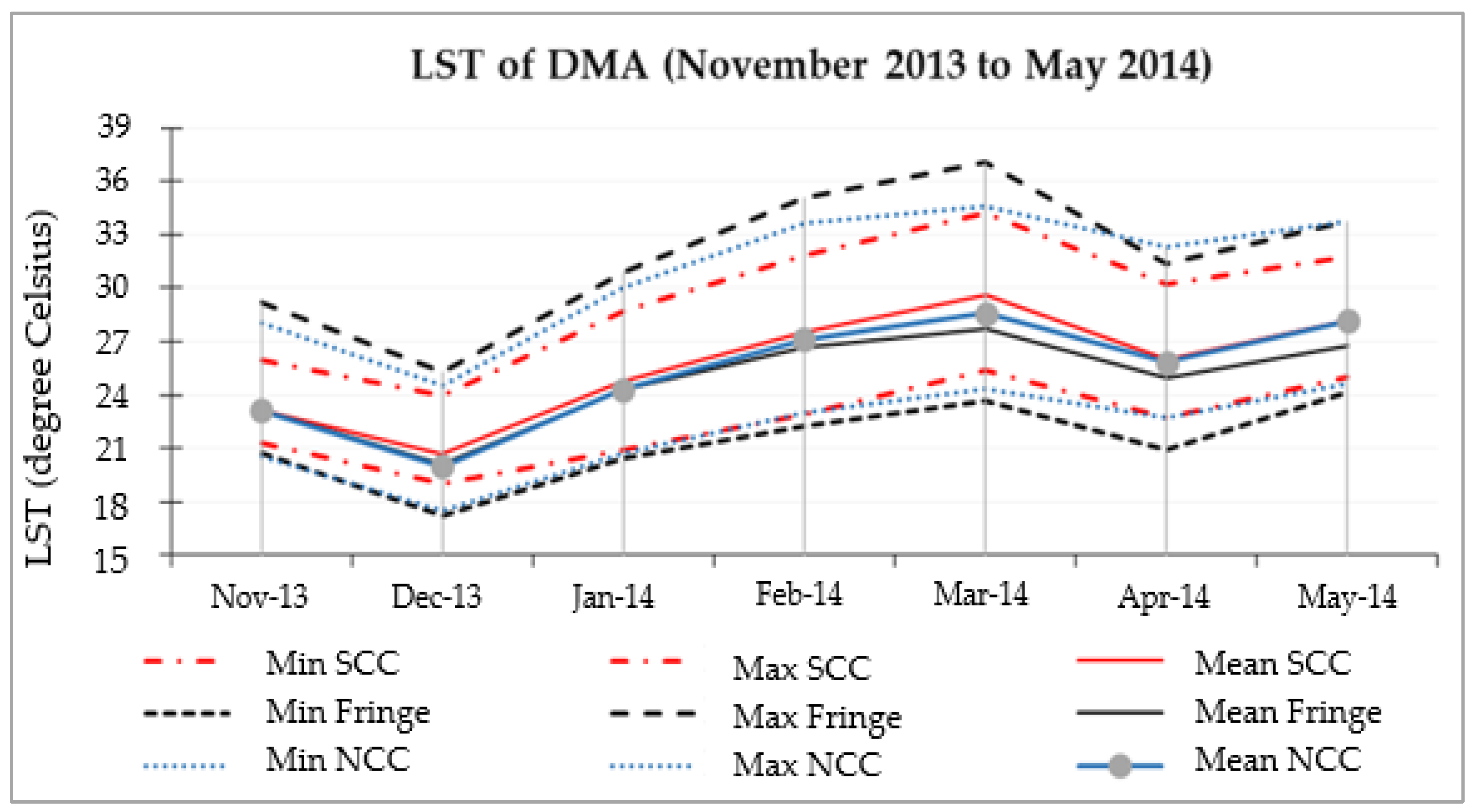
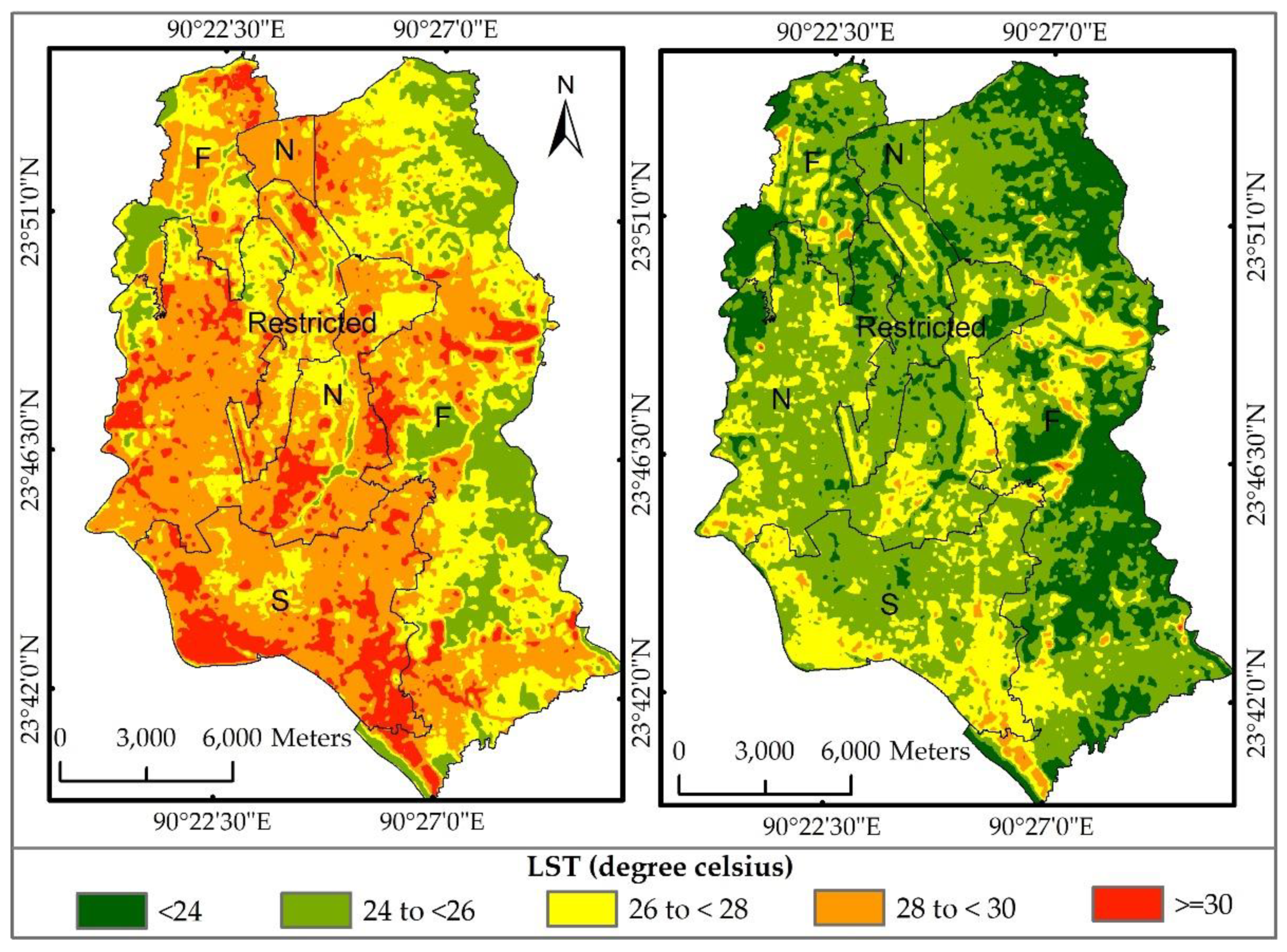
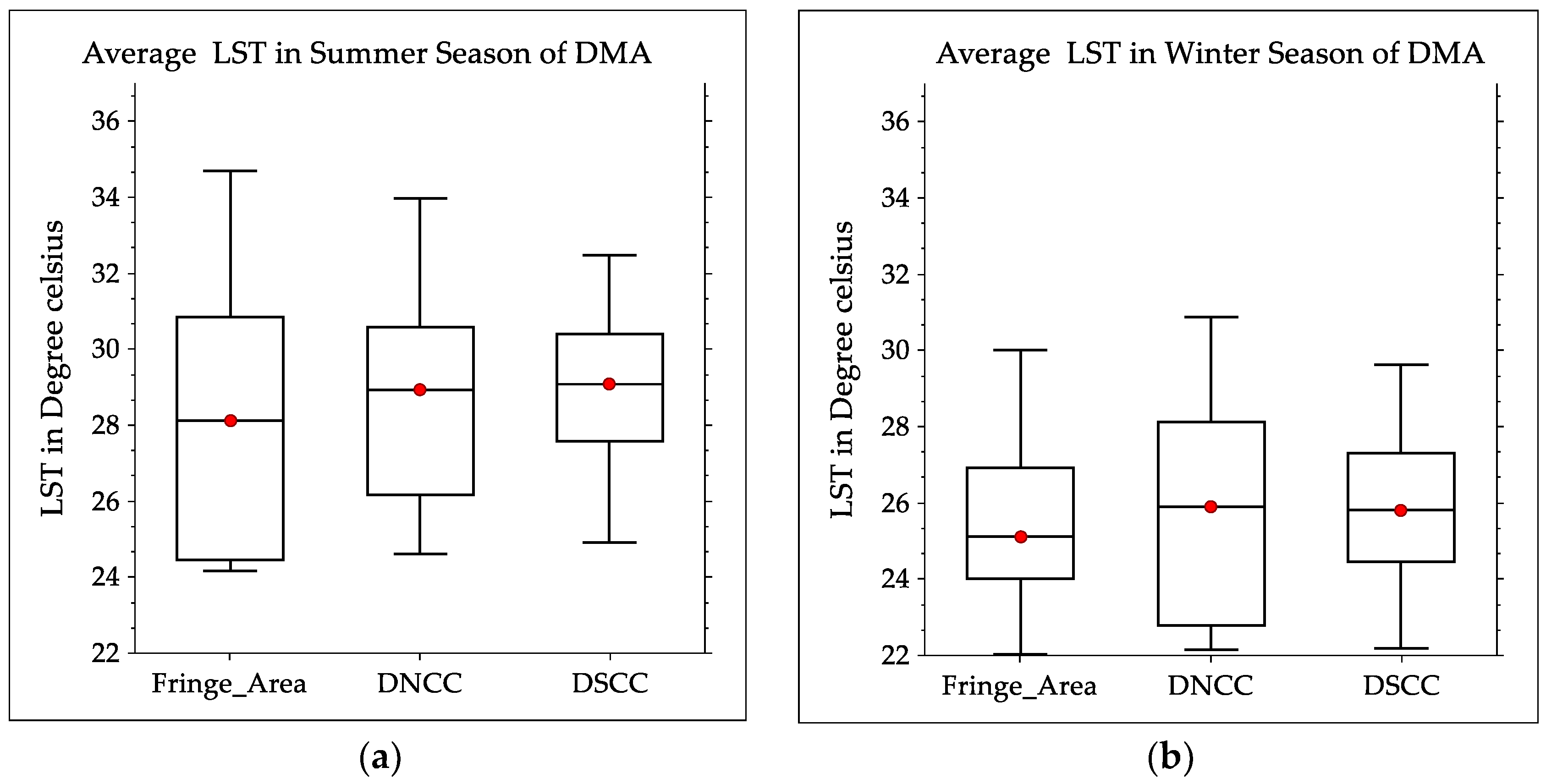
4.3. Land Surface Temperature (LST)
4.4. LST Impact Assessment
4.4.1. Correlation Analysis
4.4.2. Three-Dimensional (3D) Surface Plot
5. Discussion
6. Conclusions
Author Contributions
Funding
Acknowledgments
Conflicts of Interest
References
- Bek, M.; Azmy, N.; Elkafrawy, S. The effect of unplanned growth of urban areas on heat island phenomena. Ain Shams Eng. J. 2018, 9, 3169–3177. [Google Scholar] [CrossRef]
- Wong, N.H.; Yu, C. Study of green areas and urban heat island in a tropical city. Habitat Int. 2005, 29, 547–558. [Google Scholar] [CrossRef]
- Coutts, A.; White, E.C.; Tapper, N.; Beringer, J.; Livesley, S. Temperature and human thermal comfort effects of street trees across three contrasting street canyon environments. Theor. Appl. Clim. 2015, 124, 55–68. [Google Scholar] [CrossRef]
- Santamouris, M. Energy and Climate in the Urban Built Environment; Informa UK Limited: Colchester, UK, 2013. [Google Scholar]
- A, B.; S, L. Urban heat island effect: it’s relevance in urban planning. J. Biodivers. Endanger. Species 2017, 5, 5–187. [Google Scholar] [CrossRef]
- Guo, Z.; Wang, S.; Cheng, M.; Shu, Y. Assess the effect of different degrees of urbanization on land surface temperature using remote sensing images. Procedia Environ. Sci. 2012, 13, 935–942. [Google Scholar] [CrossRef]
- Cuberes, D. Sequential city growth: Empirical evidence. J. Urban Econ. 2011, 69, 229–239. [Google Scholar] [CrossRef]
- Naserikia, M.; Shamsabadi, E.A.; Rafieian, M.; Filho, W.L. The urban heat island in an urban context: a case study of Mashhad, Iran. Int. J. Environ. Res. Public Heal. 2019, 16, 313. [Google Scholar] [CrossRef]
- Bonafoni, S.; Keeratikasikorn, C. Land surface temperature and urban density: Multiyear modeling and relationship analysis using MODIS and Landsat data. Remote Sens. 2018, 10, 1471. [Google Scholar] [CrossRef]
- Mushore, T.D. Linking thermal variabilty and change to urban growth in harare metropolitan city using remotely sensed data. PhD Thesis, University of Zimbabwe, Harare, Zimbabwe, 15 December 2017. [Google Scholar]
- Jalan, S.; Sharma, K. Spatio-temporal assessment of land use/land cover dynamics and urban heat island of Jaipur city using satellite data. Int. Arch. Photogramm. Remote Sens. Spat. Inf. Sci. 2014, 40, 767. [Google Scholar] [CrossRef]
- Avdan, U.; Jovanovska, G. Algorithm for automated mapping of land surface temperature using LANDSAT 8 satellite data. J. Sensors 2016, 2016, 1–8. [Google Scholar] [CrossRef]
- Avtar, R.; Tripathi, S.; Aggarwal, A.K.; Kumar, P. Population–Urbanization–Energy Nexus: A Review. Resour. 2019, 8, 136. [Google Scholar] [CrossRef]
- Hung, W.-C.; Chen, Y.-C.; Cheng, K.-S. Comparing landcover patterns in Tokyo, Kyoto, and Taipei using ALOS multispectral images. Landsc. Urban Plan. 2010, 97, 132–145. [Google Scholar] [CrossRef]
- Avtar, R.; Aggarwal, R.; Kharrazi, A.; Kumar, P.; Kurniawan, T.A. Utilizing geospatial information to implement SDGs and monitor their Progress. Environ. Monit. Assess. 2020, 192, 35. [Google Scholar] [CrossRef] [PubMed]
- Ferdous Jannatul, R.T. Temporal Dynamics and Relationship of Land Use Land Cover and Land Surface Temperature in Dhaka. In Proceedings of the 4th International Conference on Civil Engineering for Sustainable Development (ICCESD 2018), KUET, Khulna, Bangladesh, 9–11 February 2018. [Google Scholar]
- Alobeid, A.; Jacobsen, K.; Heipke, C. Comparison of matching algorithms for DSM generation in urban areas from Ikonos imagery. Photogramm. Eng. Remote Sens. 2010, 76, 1041–1050. [Google Scholar] [CrossRef]
- Avtar, R.; Sawada, H. Use of DEM data to monitor height changes due to deforestation. Arab. J. Geosci. 2012, 6, 4859–4871. [Google Scholar] [CrossRef]
- Buyantuyev, A.; Wu, J. Urban heat islands and landscape heterogeneity: linking spatiotemporal variations in surface temperatures to land-cover and socioeconomic patterns. Landsc. Ecol. 2009, 25, 17–33. [Google Scholar] [CrossRef]
- Arnfield, A.J. Two decades of urban climate research: a review of turbulence, exchanges of energy and water, and the urban heat island. Int. J. Clim. 2003, 23, 1–26. [Google Scholar] [CrossRef]
- Ramaiah, M.; Avtar, R. Urban green spaces and their need in cities of rapidly urbanizing India: A review. Urban Sci. 2020, 3, 94. [Google Scholar] [CrossRef]
- Grover, A.; Singh, R. Analysis of urban heat island (UHI) in relation to normalized difference vegetation index (NDVI): A comparative study of Delhi and Mumbai. Environ. 2015, 2, 125–138. [Google Scholar] [CrossRef]
- Groleau, D.; Mestayer, P.G. Urban Morphology Influence on Urban Albedo: A Revisit with the S olene Model. Boundary-layer Meteorol. 2013, 147, 301–327. [Google Scholar] [CrossRef]
- Taha, H. Urban climates and heat islands: albedo, evapotranspiration, and anthropogenic heat. Energy Build. 1997, 25, 99–103. [Google Scholar] [CrossRef]
- Yuan, J.; Emura, K.; Farnham, C. Is urban albedo or urban green covering more effective for urban microclimate improvement?: A simulation for Osaka. Sustain. Cities Soc. 2017, 32, 78–86. [Google Scholar] [CrossRef]
- Maimaitiyiming, M.; Ghulam, A.; Tiyip, T.; Pla, F.; Latorre-Carmona, P.; Halik, Ü.; Sawut, M.; Caetano, M. Effects of green space spatial pattern on land surface temperature: Implications for sustainable urban planning and climate change adaptation. ISPRS J. Photogramm. Remote Sens. 2014, 89, 59–66. [Google Scholar] [CrossRef]
- Dousset, B.; Gourmelon, F. Satellite multi-sensor data analysis of urban surface temperatures and landcover. ISPRS J. Photogramm. Remote Sens. 2003, 58, 43–54. [Google Scholar] [CrossRef]
- Cao, L.; Li, P.; Zhang, L.; Chen, T. Remote sensing image-based analysis of the relationship between urban heat island and vegetation fraction. Int. Arch. Photogramm. Remote Sens. Spat. Inf. Sci. 2008, 37. [Google Scholar]
- Bowler, D.E.; Buyung-Ali, L.; Knight, T.M.; Pullin, A. Urban greening to cool towns and cities: A systematic review of the empirical evidence. Landsc. Urban Plan. 2010, 97, 147–155. [Google Scholar] [CrossRef]
- Abraham, S. The relevance of wetland conservation in Kerala. Int. J. Fauna Biol. Stud. 2015, 2, 1–5. [Google Scholar]
- Zhang, W.; Li, W.; Zhang, C.; Ouimet, W.B. Detecting horizontal and vertical urban growth from medium resolution imagery and its relationships with major socioeconomic factors. Int. J. Remote Sens. 2017, 38, 3704–3734. [Google Scholar] [CrossRef]
- Yang, C.; He, X.; Wang, R.; Yan, F.; Yu, L.; Bu, K.; Yang, J.; Chang, L.; Zhang, S. The effect of urban green spaces on the urban thermal environment and its seasonal variations. For. 2017, 8, 153. [Google Scholar] [CrossRef]
- Ranagalage, M.; Estoque, R.C.; Murayama, Y. An urban heat island study of the Colombo metropolitan area, Sri Lanka, based on Landsat data (1997–2017). ISPRS Int. J. Geo-Information 2017, 6, 189. [Google Scholar] [CrossRef]
- Avtar, R.; Kumar, P.; Oono, A.; Saraswat, C.; Dorji, S.; Hlaing, Z. Potential application of remote sensing in monitoring ecosystem services of forests, mangroves and urban areas. Geocarto Int. 2017, 32, 874–885. [Google Scholar] [CrossRef]
- Gage, E.A.; Cooper, D.J. Relationships between landscape pattern metrics, vertical structure and surface urban Heat Island formation in a Colorado suburb. Urban Ecosyst. 2017, 20, 1–1238. [Google Scholar] [CrossRef]
- Hofierka, J.; Gallay, M.; Onačillová, K.; Hofierka, J. Urban Climate Physically-based land surface temperature modeling in urban areas using a 3-D city model and multispectral satellite data. Urban Clim. 2020, 31, 100566. [Google Scholar] [CrossRef]
- Mia, B.; Bhattacharya, R.; Woobaidullah, A.S.M. Correlation and Monitoring of Land Surface Temperature, Urban Heat Island with Land use-land cover of Dhaka City using Satellite imageries. Int. J. Res. Geogr. 2017, 3, 10–20. [Google Scholar]
- Han, G.; Xu, J. Land surface phenology and land surface temperature changes along an urban–rural gradient in Yangtze River Delta, China. Environ. Manag. 2013, 52, 234–249. [Google Scholar] [CrossRef] [PubMed]
- Ahmed, B.; Kamruzzaman, M.; Zhu, X.; Rahman, M.; Choi, K. Simulating land cover changes and their impacts on land surface temperature in Dhaka, Bangladesh. Remote Sens. 2013, 5, 5969–5998. [Google Scholar] [CrossRef]
- Hossain, S. Rapid Urban Growth and Poverty in Dhaka City. Bangladesh e-journal Sociol. 2008, 5, 1–24. [Google Scholar]
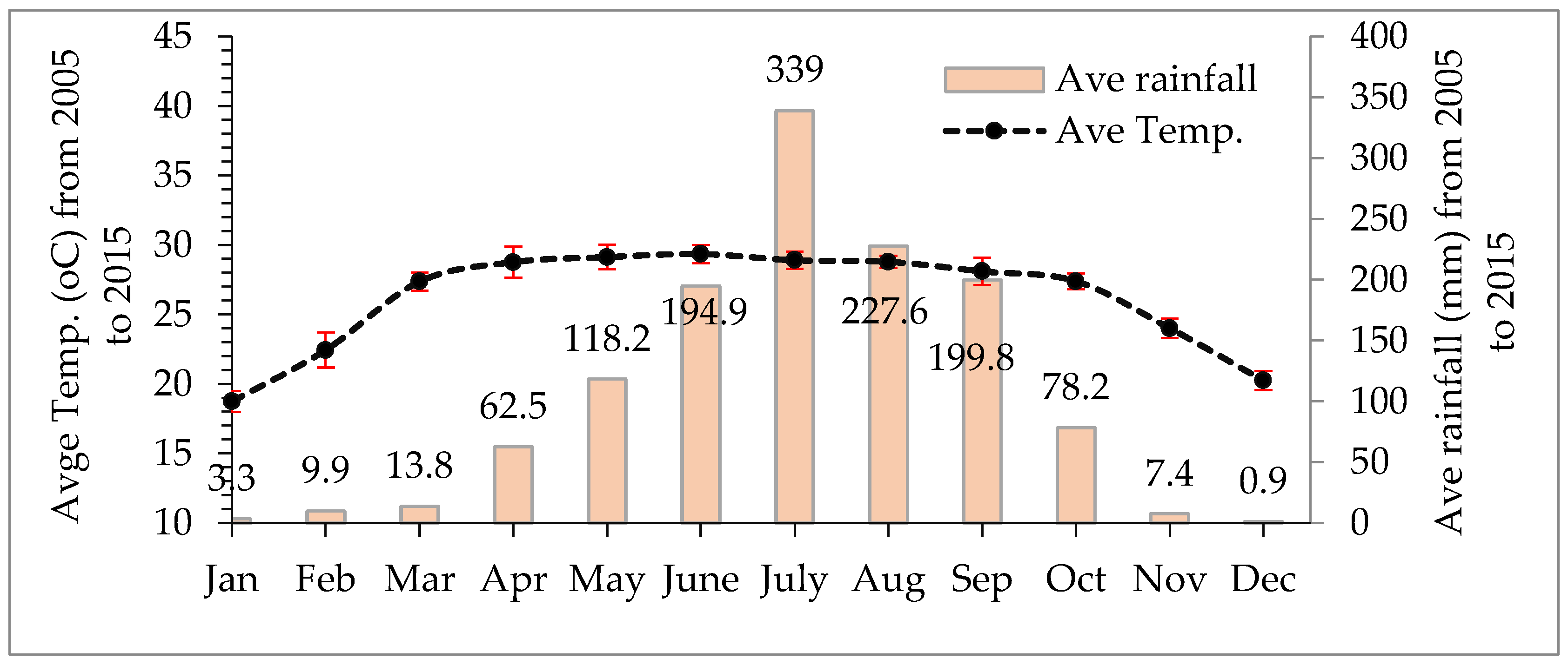
- Shahid, S. Recent trends in the climate of Bangladesh. Clim. Res. 2010, 42, 185–193. [Google Scholar] [CrossRef]
- Hordijk, M.; Baud, I. Resilient Cities: Cities and adaptation to climate change. Media 2011, 1, 111–121. [Google Scholar]
- Raja, D.R. Spatial analysis of land surface temperature in Dhaka metropolitan area. J Bangladesh Inst. Plann ISSN 2012, 2075, 9363. [Google Scholar]
- Kosmann, D.; Wessel, B.; Schwieger, V. Global digital elevation model from TanDEM-X and the calibration/validation with worldwide kinematic GPS-tracks. In Proceedings of the FIG Congress, Sydney, Australia, 11–16 April 2010. [Google Scholar]
- Rott, H.; Floricioiu, D.; Wuite, J.; Scheiblauer, S.; Nagler, T.; Kern, M. Mass changes of outlet glaciers along the Nordensjköld Coast, northern Antarctic Peninsula, based on TanDEM-X satellite measurements. Geophys. Res. Lett. 2014, 41, 8123–8129. [Google Scholar] [CrossRef]
- Hojo, A.; Takagi, K.; Avtar, R.; Tadono, T.; Nakamura, F. Synthesis of L-Band SAR and Forest Heights Derived from TanDEM-X DEM and 3 Digital Terrain Models for Biomass Mapping. Remote Sens. 2020, 12, 349. [Google Scholar] [CrossRef]
- Wessel, B.; Huber, M.; Wohlfart, C.; Marschalk, U.; Kosmann, D.; Roth, A. Accuracy assessment of the global TanDEM-X Digital Elevation Model with GPS data. ISPRS J. Photogramm. Remote Sens. 2018, 139, 171–182. [Google Scholar] [CrossRef]
- Avtar, R.; Yunus, A.P.; Kraines, S.; Yamamuro, M. Evaluation of DEM generation based on Interferometric SAR using TanDEM-X data in Tokyo. Physics and Chemistry of the Earth, Parts A/B/C. 2015, 83, 166–177. [Google Scholar] [CrossRef]
- Tachikawa, T.; Kaku, M.; Iwasaki, A.; Gesch, D.B.; Oimoen, M.J.; Zhang, Z.; Danielson, J.J.; Krieger, T.; Curtis, B.; Haase, J. ASTER global digital elevation model version 2-summary of validation results; NASA: Washington, DC, USA, 2011.
- Gesch, D.; Oimoen, M.; Zhang, Z.; Danielson, J.; Meyer, D. Validation of the ASTER Global Digital Elevation Model (GDEM) Version 2 over the Conterminous United States. Rep. to ASTER GDEM Version 2011, 2, 281–286. [Google Scholar]
- Santillan, J.R.; Makinano-Santillan, M. Vertical accuracy assessment of 30-m resolution alos, aster, and srtm global dems over northeastern mindanao, philippines. Int. Arch. Photogramm. Remote Sens. Spat. Inf. Sci. 2016, 41, 149–156. [Google Scholar] [CrossRef]
- Rahman, M.S.; Di, L. The state of the art of spaceborne remote sensing in flood management. Nat. Hazards 2017, 85, 1223–1248. [Google Scholar] [CrossRef]
- Takaku, J.; Tadono, T. PRISM geometric validation and DSM generation status. In Proceedings of the The First Joint PI Symposium of ALOS Data Nodes for ALOS Science Program, Kyoto, Japan, 19–23 November 2007. [Google Scholar]
- Sekertekin, A.; Marangoz, A.M.; Akcin, H. Pixel-based classification analysis of land use land cover using Sentinel-2 and Landsat-8 data. Int. Arch. Photogramm. Remote Sens. Spat. Inf. Sci. 2017, 42, 91–93. [Google Scholar] [CrossRef]
- Barsi, J.; Schott, J.; Hook, S.; Raqueno, N.; Markham, B.; Radocinski, R. Landsat-8 thermal infrared sensor (TIRS) vicarious radiometric calibration. Remote Sens. 2014, 6, 11607–11626. [Google Scholar] [CrossRef]
- Yu, X.; Guo, X.; Wu, Z. Land surface temperature retrieval from Landsat 8 TIRS—Comparison between radiative transfer equation-based method, split window algorithm and single channel method. Remote Sens. 2014, 6, 9829–9852. [Google Scholar] [CrossRef]
- Rajeshwari, A.; Mani, N.D. Estimation of land surface temperature of Dindigul district using Landsat 8 data. Int. J. Res. Eng. Technol. 2014, 3, 122–126. [Google Scholar]
- Tahar, K.N. An evaluation on different number of ground control points in unmanned aerial vehicle photogrammetric block. Int. Arch. Photogramm. Remote Sens. Spat. Inf. Sci 2013, 40, 93–98. [Google Scholar] [CrossRef]
- Abdul-Rahman, A.; Zlatanova, S.; Coors, V. Innovations in 3D geo information systems; Springer Science & Business Media: Berlin, Heidelberg, 2007; ISBN 3540369988. [Google Scholar]
- Courty, L.; Soriano-Monzalvo, J.C.; Pedrozo-Acuña, A. Evaluation of open-access global digital elevation models (AW3D30, SRTM and ASTER) for flood modelling purposes. J. Flood Risk Manag. 2019, 12, e12550. [Google Scholar] [CrossRef]
- Apeh, O.I.; Uzodinma, V.N.; Ebinne, E.S.; Moka, E.C.; Onah, E.U. Accuracy Assessment of Alos W3d30, Aster Gdem and Srtm30 Dem: A Case Study of Nigeria, West Africa. J. Geogr. Inf. Syst. 2019, 11, 111–123. [Google Scholar] [CrossRef][Green Version]
- Akristiniy, V.A.; Boriskina, Y.I. Vertical cities-the new form of high-rise construction evolution. In Proceedings of the E3S Web of Conferences; EDP Sciences: Julius, France, 2018; Volume 33, p. 1041. [Google Scholar]
- Özcan, A.H.; Ünsalan, C.; Reinartz, P. Ground filtering and DTM generation from DSM data using probabilistic voting and segmentation. Int. J. Remote Sens. 2018, 39, 2860–2883. [Google Scholar] [CrossRef]
- Gevaert, C.M.; Persello, C.; Nex, F.; Vosselman, G. A deep learning approach to DTM extraction from imagery using rule-based training labels. ISPRS J. Photogramm. Remote Sens. 2018, 142, 106–123. [Google Scholar] [CrossRef]
- Xiaogang, N.; Qin, Y.; Yang, B. Extracting and analyzing urban built-up area based on impervious surface and gravity model. In Proceedings of the Joint Urban Remote Sensing Event 2013; IEEE, Sao Paulo, Brazil, 21–23 April 2013. [Google Scholar]
- Phiri, D.; Morgenroth, J. Developments in Landsat land cover classification methods: A review. Remote Sens. 2017, 9, 967. [Google Scholar] [CrossRef]
- Cortes, C.; Vapnik, V. Support-vector networks. Mach. Learn. 1995, 20, 273–297. [Google Scholar] [CrossRef]
- Shao, Y.; Lunetta, R.S. Comparison of support vector machine, neural network, and CART algorithms for the land-cover classification using limited training data points. ISPRS J. Photogramm. Remote Sens. 2012, 70, 78–87. [Google Scholar] [CrossRef]
- Zhang, T.; Tang, H. A Comprehensive evaluation of approaches for built-up area extraction from Landsat OLI images using massive samples. Remote Sens. 2019, 11. [Google Scholar] [CrossRef]
- Li, Z.-L.; Tang, B.-H.; Wu, H.; Ren, H.; Yan, G.; Wan, Z.; Trigo, I.F.; Sobrino, J.A. Satellite-derived land surface temperature: Current status and perspectives. Remote Sens. Environ. 2013, 131, 14–37. [Google Scholar] [CrossRef]
- Kahle, A.B.; Morrison, A.D.; Tsu, H.; Yamaguchi, Y. Geologic remote sensing in the thermal infrared. In Proceedings of the New technology for geosciences: proceedings of the 30th International Geological Congress, Beijing, China, 4–14 August 1996. [Google Scholar]
- Morshed, N.; Yorke, C.; Zhang, Q. Urban expansion pattern and land use dynamics in Dhaka, 1989–2014. Prof. Geogr. 2017, 69, 396–411. [Google Scholar] [CrossRef]
- Singh, R.; Grover, A.; Zhan, J. Inter-seasonal variations of surface temperature in the urbanized environment of Delhi using Landsat thermal data. Energies 2014, 7, 1811–1828. [Google Scholar] [CrossRef]
- Gallo, K.; Hale, R.; Tarpley, D.; Yu, Y. Evaluation of the relationship between air and land surface temperature under clear- and cloudy-sky conditions. J. Appl. Meteorol. Clim. 2011, 50, 767–775. [Google Scholar] [CrossRef]
- Guo, G.; Zhou, X.; Wu, Z.; Xiao, R.; Chen, Y. Characterizing the impact of urban morphology heterogeneity on land surface temperature in Guangzhou, China. Environ. Model. Softw. 2016, 84, 427–439. [Google Scholar] [CrossRef]
- Guo, G.; Wu, Z.; Xiao, R.; Chen, Y.; Liu, X.; Zhang, X. Impacts of urban biophysical composition on land surface temperature in urban heat island clusters. Landsc. Urban Plan. 2015, 135, 1–10. [Google Scholar] [CrossRef]
- Ruffieux, D.; Wolfe, D.E.; Russell, C. The effect of building shadows on the vertical temperature structure of the lower atmosphere in downtown Denver. J. Appl. Meteorol. 1990, 29, 1221–1231. [Google Scholar] [CrossRef]
- Zheng, Z.; Zhou, W.; Yan, J.; Qian, Y.; Wang, J.; Li, W. The higher, the cooler? Effects of building height on land surface temperatures in residential areas of Beijing. Phys. Chem. Earth Parts A/B/C 2019, 110, 149–156. [Google Scholar] [CrossRef]
- Peng, F.; Gong, J.; Wang, L.; Wu, H.; Yang, J. Impact of building heights on 3d urban density estimation from spaceborne stereo imagery. Int. Arch. Photogramm. Remote Sens. Spat. Inf. Sci. - ISPRS Arch. 2016, 41, 677–683. [Google Scholar] [CrossRef]
- Misra, P.; Avtar, R.; Takeuchi, W. Comparison of Digital Building Height Models Extracted from AW3D, TanDEM-X, ASTER, and SRTM Digital Surface Models over Yangon City. Remote Sens. 2018, 10, 2008. [Google Scholar] [CrossRef]
- Cai, M.; Ren, C.; Xu, Y.; Lau, K.K.L.; Wang, R. Investigating the relationship between local climate zone and land surface temperature using an improved WUDAPT methodology—A case study of Yangtze River Delta, China. Urban Clim. 2018, 24, 485–502. [Google Scholar] [CrossRef]
- Wang, R.; Cai, M.; Ren, C.; Bechtel, B.; Xu, Y.; Ng, E. Detecting multi-temporal land cover change and land surface temperature in Pearl River Delta by adopting local climate zone. Urban Clim. 2019, 28, 100455. [Google Scholar] [CrossRef]
- Chen, F.; Yang, S.; Yin, K.; Chan, P. Challenges to quantitative applications of Landsat observations for the urban thermal environment. J. Environ. Sci. 2017, 59, 80–88. [Google Scholar] [CrossRef] [PubMed]
- Xu, H. Analysis of impervious surface and its impact on urban heat environment using the normalized difference impervious surface index (NDISI). Photogramm. Eng. Remote Sens. 2010, 76, 557–565. [Google Scholar] [CrossRef]
- Yang, J.; Wong, M.-S.; Ho, H.C. Retrieval of Urban Surface Temperature Using Remote Sensing Satellite Imagery. In Big Data for Remote Sensing: Visualization, Analysis and Interpretation; Springer: Basel, Switzerland, 2018. [Google Scholar]


| Data | Acquisition | Vertical Accuracy * | Imaging System | Resolution (m) | Sources |
|---|---|---|---|---|---|
| TanDEM-X | 16 October 2012 | 1.6–6.2 m | SAR X band | 12 | German Aerospace Center, DLR |
| ASTER (GDEM V2), publicly released 2011 | 2009 | 15.1–23.2 m | Optical | 30 | US Geological Survey (USGS), |
| AW3D30 Publicly released by JAXA in 2015 | 2006-2011 | 1.7–6.8 m | Optical | 30 | Japan Aerospace Exploration Agency (JAXA) |
| Path/Tiles | Acquisition Date | Local Acquisition Time (am) | Band | Source | Remarks |
|---|---|---|---|---|---|
| Landsat-8 OLI WRS-2, 137/44 | 06-11-13 | 10:26:34.15 | Band (3,4,5,6) 30m and TIR band (10,11) 100m | US Geological Survey (USGS), | TIR band for LST retrieval and other bands for Land Use Land Cover (LULC) mapping |
| 24-12-13 | 10:26:16.33 | ||||
| 25-01-14 | 10:25:56.73 | ||||
| 06-02-14 | 10:25:31.49 | ||||
| 14-03-14 | 10:25:20.51 | ||||
| 24-04-14 | 10:25:51.49 | ||||
| 06-05-14 | 10:26:01.49 |
| Land Cover Types | Description |
|---|---|
| Built-up area | All infrastructure, settlement, road |
| Bare Land | Fallow land, dry soil, sand filling |
| Non-built-up area | Natural vegetation, parks, agricultural land, wetland, pond, canal, river, marshy land |
| Low Density (<40%) | Medium Density (40% to <70%) | High Density (>70%) | |
|---|---|---|---|
| Low height (2.5 m to <19.6 m) | 11% | 38% | 35% |
| Medium height (19.6 to <52.48m) | 1% | 7.5% | 7% |
| High height (>52.8m) | 0.05% | 0.07% | 0.12% |
| Building Height/Built-Up Density/ Mean LST | Built-Up Density | ||||||
|---|---|---|---|---|---|---|---|
| High | Medium | Low | High | Medium | Low | ||
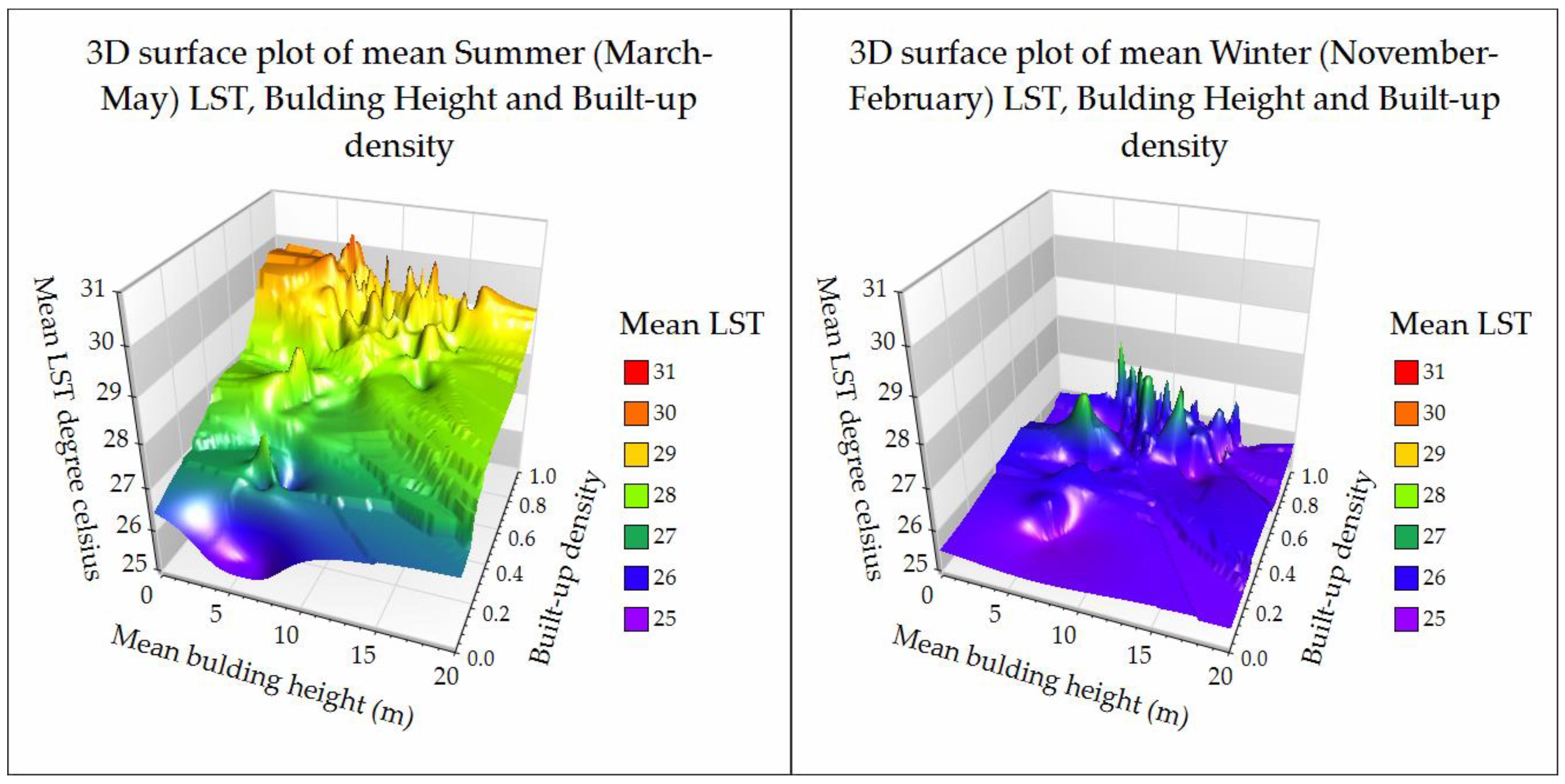
| Summer LST | Winter LST | ||||||
| Building Height | High | 29.32 °C | 29.28 °C | 29.15 °C | 28.03 °C | 27.67 °C | 27.38 °C |
| Medium | 29.96 °C | 29.42 °C | 29.12 °C | 28.08 °C | 27.57 °C | 27.61 °C | |
| Low | 30.24 °C | 29.33 °C | 28.41 °C | 28.32 °C | 27.85 °C | 26.77 °C | |
© 2020 by the authors. Licensee MDPI, Basel, Switzerland. This article is an open access article distributed under the terms and conditions of the Creative Commons Attribution (CC BY) license (http://creativecommons.org/licenses/by/4.0/).
Share and Cite
Rahman, M.M.; Avtar, R.; Yunus, A.P.; Dou, J.; Misra, P.; Takeuchi, W.; Sahu, N.; Kumar, P.; Johnson, B.A.; Dasgupta, R.; et al. Monitoring Effect of Spatial Growth on Land Surface Temperature in Dhaka. Remote Sens. 2020, 12, 1191. https://doi.org/10.3390/rs12071191
Rahman MM, Avtar R, Yunus AP, Dou J, Misra P, Takeuchi W, Sahu N, Kumar P, Johnson BA, Dasgupta R, et al. Monitoring Effect of Spatial Growth on Land Surface Temperature in Dhaka. Remote Sensing. 2020; 12(7):1191. https://doi.org/10.3390/rs12071191
Chicago/Turabian StyleRahman, Md. Mustafizur, Ram Avtar, Ali P. Yunus, Jie Dou, Prakhar Misra, Wataru Takeuchi, Netrananda Sahu, Pankaj Kumar, Brian Alan Johnson, Rajarshi Dasgupta, and et al. 2020. "Monitoring Effect of Spatial Growth on Land Surface Temperature in Dhaka" Remote Sensing 12, no. 7: 1191. https://doi.org/10.3390/rs12071191
APA StyleRahman, M. M., Avtar, R., Yunus, A. P., Dou, J., Misra, P., Takeuchi, W., Sahu, N., Kumar, P., Johnson, B. A., Dasgupta, R., Kharrazi, A., Chakraborty, S., & Agustiono Kurniawan, T. (2020). Monitoring Effect of Spatial Growth on Land Surface Temperature in Dhaka. Remote Sensing, 12(7), 1191. https://doi.org/10.3390/rs12071191