Abstract
Orthorectification is an important step in generating accurate land use/land cover (LULC) from satellite imagery, particularly in urban areas with high-rise buildings. Such buildings generally appear as oblique shapes on very-high-resolution (VHR) satellite images, which reflect a bigger area of coverage than the real built-up area on LULC mapping. This drawback can cause not only uncertainties in urban mapping and LULC classification, but can also result in inaccurate urban change detection. Overestimating volume or area of high-rise buildings has a negative impact on computing the exact amount of environmental heat and emission. Hence, in this study, we propose a method of orthorectfiying VHR WorldView-3 images by integrating light detection and ranging (LiDAR) data to overcome the aforementioned problems. A 3D rational polynomial coefficient (RPC) model was proposed with respect to high-accuracy ground control points collected from the LiDAR data derived from the digital surface model. Multiple probabilities for generating an orthrorectified image from WV-3 were assessed using 3D RCP model to achieve the optimal combination technique, with low vertical and horizontal errors. Ground control point (GCPs) collection is sensitive to variation in number and data collection pattern. These steps are important in orthorectification because they can cause the morbidity of a standard equation, thereby interrupting the stability of 3D RCP model by reducing the accuracy of the orthorectified image. Hence, we assessed the maximum possible scenarios of resampling and ground control point collection techniques to bridge the gap. Results show that the 3D RCP model accurately orthorectifies the VHR satellite image if 20 to 100 GCPs were collected by convenience pattern. In addition, cubic conventional resampling algorithm improved the precision and smoothness of the orthorectified image. According to the root mean square error, the proposed combination technique enhanced the vertical and horizontal accuracies of the geo-positioning process to up to 0.8 and 1.8 m, respectively. Such accuracy is considered very high in orthorectification. The proposed technique is easy to use and can be replicated for other VHR satellite and aerial photos.
1. Introduction
The rapid expansion of remote sensing technologies has greatly upgraded the spectral and spatial resolutions of remotely sensed images [1,2]. Very-high-resolution (VHR) remote sensing images are recent spatial datasets used to build the digital Earth from where the digitized information from earth features can be extracted. They can be broadly utilised in different areas or subjects, such as land use modelling, agriculture, natural hazard, urban planning and forestry [3,4,5]. Such datasets are specifically applied in disaster emergency monitoring (soil erosion and urban flash flooding), monitoring of land cover and settlement monitoring [6,7,8,9,10].
VHR satellite image possessing involves precise and timely feature extraction. It offers quick data collection, no geographic limitation, moderate to low cost and plenty of texture and geospatial information. Thus, the use of VHR image processing methods in numerous applications have persistently received attention [11,12]. Several studies have investigated the multiple applications of recent VHR imagery [3,4,13,14]. Nevertheless, an accurate and operational image processing technique that can identify and retrieve beneficial information from processed imagery automatically and quickly is yet to be achieved [15]. Implementing orthorectification models in the processing of VHR imageries is an essential phase in achieving highly accurate orthorectification of remote sensing images [16]. Apart from establishing a mathematical orthorectification model of a satellite image, the mathematical association with 3D spatial coordinates of ground control points (GCPs) and the corresponding pixel of image points can be highlighted [17].
The orthorectification of VHR satellite image is one of the essential preprocessing phases for precise recognition of broad urban objects [12]. WorldView-3 (WV-3) satellite is a commercial VHR satellite that captures images with the finest spatial resolution of 0.31 m at nadir in panchromatic (PAN) band. The off-nadir angle of the VHR satellites can capture panchromatic (PAN) band lower than 0.5 m; hence, they should be orthorectified by GCPs [18]. VHR imagery is currently available as (i) basic image or (ii) projected image to a plane with constant elevation level. This imagery can be orthorectified accurately by end-users using image-processing software and ancillary dataset, such as GCPs or digital elevation models (DEMs), through VHR satellite imagery. DigitalGlobe’s VHR images are generally available in basic products which ought to implement orthorectification and map registration [19].
The key stage for the orthorectification is sensor orientation or triangulation, through which the final product is produced by removal of the negative distorting effects on the terrain relief. In recent decades, numerous mathematical models for VHR satellite sensor orientation and geo-positioning using GCPs have been investigated to correct geometric distortions from imagery [20,21]. Those models can be generally classified as physical and deterministic or empirical, whereas each class can be represented in 2D or 3D method [20].
Rigorous or physical models identify the relationship between the captured image and the satellite image on the ground according to the satellite sensor motion [16]. The quality of such models relies on the quality and availability of the satellite ephemeris and sensor metadata [22]. However, the mathematical type of rigorous models might vary from one sensor to another. A physical model is based on standard photogrammetric methodology, where the collinearity calculations connect the ground coordinates with the satellite image [22]. A physical model must see the ground’s morphological characteristics, such as attitude and velocity; sensor specifications like panoramic effect; the angle of view; and coordinate systems, such as ellipsoid and 3D relief [23].
Empirical models generally estimate the relationship between the target objects and satellite image with less information about the satellite ephemeris and motion in space [18]. Numerous researchers suggest the use of rational functions models (RFMs) as mathematical models in the absence of sensor metadata for ground coordinate system transformation [21,24,25]. Such empirical models can be applied directly when acquisition system information is not available. In addition, they are calculated using multiple mathematical function dimensions (e.g., 3D rational functions, 2D or 3D polynomial functions) [26]. The correlation between the coordinates of points on the satellite imagery and their equivalent points on the ground are characterised by polynomial functions. The constants of the polynomial can be calculated using a sufficient number of GCPs with benchmark locations on the thematic map and recognisable of the image [27].
The object spaces and satellite image can be matched via a ratio of polynomial functions to calculate the image column and row [28]. A sufficient number of GCPs with high vertical and horizontal precision is needed to compute the coefficients of polynomials called rational polynomial coefficients (RPCs); RPCs are well-adopted models with third-order parameters [18,28,29]. Therefore, height information for GCPs can be mined from digital surface models (DSMs) and topographic or GPS surveys. Comprehensive topographical maps (scale 1:5000 or finer) and remotely sensed imagery with the similar spatial resolution of the PAN band of an orthorectified satellite image, such as light detection and ranging (LiDAR) dataset, are appropriate for extracting horizontal and vertical coordinates for GCPs. The 2D Polynomial functions are not perfect systems to orthorectify VHR images because these imageries did not consider the effects of ground elevation which must be corrected for basic planimetric distortion at the GCPs [30,31].
Empirical and physical models are applied in 2D and 3D format to orthorectify VHR satellite imagery. Chmiel, Kay and Spruyt [12] compared such models rigorously with RFM models to obtain the best geometric accuracy of orthorectification using EROS 1A level, QuickBird and IKONOS satellites. Wolniewicz [32] assessed the impact of the distribution of GCPs on the horizontal accuracy using different orthorectification models from IKONOS and QuickBird satellite imagery. Afify and Zhang [33] evaluated the acceptable geometric accuracy using the RFMs from Quickbird and IKONOS satellite imagery. Aguilar, del Mar Saldana and Aguilar [19] compared the refined 3D RFM, the 3D Toutin physical and the first order polynomial models to find the best method for orthorectifying IKONOS and QuickBird imagery. The impact of the amount of GCPs on the geometric accuracy via the RFM model from a GeoEye-1 satellite image was assessed by [34].
Capaldo, et al. [35] compared two rigorous models using WorldView-1 and GeoEye-1. In both cases, the RFM sensor orientation model attained superior results to a 3D physical model. Nonetheless, their outputs were only supported with a low number of checkpoints without considering the GCP selection pattern.
This research is the first try to orthorectify the VHR WV-3 with respect to LiDAR DSM. It uses a 3D RCP model that considers GCP quantities, patterns and resampling methods. The main objective of this paper is to compare the vertical and horizontal accuracy of geo-positioning of WV-3 PAN single band image based on LiDAR elevation data for generating orthorectified imagery. Vertical and horizontal accuracies were assessed via statistical analysis in the following variation sources: (i) pattern of GCP collection from LiDAR DSM, (ii) number of GCPs used in the triangulation process and (iii) resampling algorithms of in the orthorectification process.
2. Study Site and Dataset
2.1. Study Site
The study areas are situated at Damansara in the Selangor State of Malaysia, which typically consists of multiple urban features, such as high-rise industrial or residential buildings with 24.02 ha area. This site was selected mainly because of the presence of high-rise buildings. The highest building of the study area has 100 m elevation from the terrain. The study area is situated at 3°8′45.6 latitude and 101°32′27.24 longitude (Figure 1).
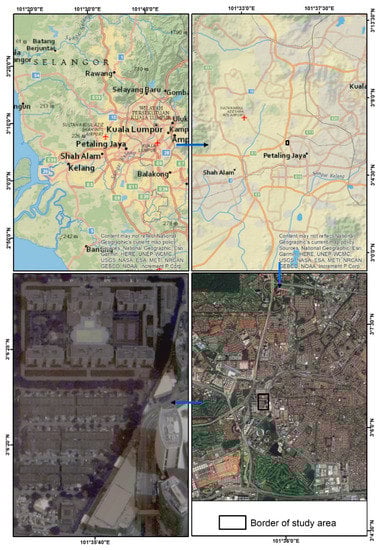
Figure 1.
The geographical location of this study.
2.2. Wordview-3 Satellite Image
A WV-3 image captured on 9 December 2015 was processed in this study. It is one of the available commercial VHR satellite images that have eight informative spectral bands (Table 1).

Table 1.
Spectral information of WV-3 image.
2.3. Airborne LiDAR Data
LiDAR data point clouds were collected on 2 November 2015 using Optech Airborne Laser Terrain Mapper 3100 with a flying height of 1510 m in clear skies. The point density is closely 8 points per square meter, with a 25,000 Hz pulse rate frequency. According to the point spacing, the data accuracy is 0.3 m. The digital surface elevation model in a raster format was extracted from LiDAR point clouds by using Arc map 10.4. The point clouds were converted to raster from LAS format by using the conversion tool. Outlier noises were then eliminated to prepare for registration with WV-3 image.
3. Methodology
The overall computational methodology applied in this study is shown in Figure 2. At first, the PAN band of WV-3 is registered with LiDAR DSM at 0.3 spatial resolution. Both datasets were geometrically corrected. To create the 3D RCP model, 3D GCPs should be collected accordingly. We examined the influence of GCP pattern, GCP number and resampling algorithms on the vertical and horizontal accuracies of orthorectified WV-3.
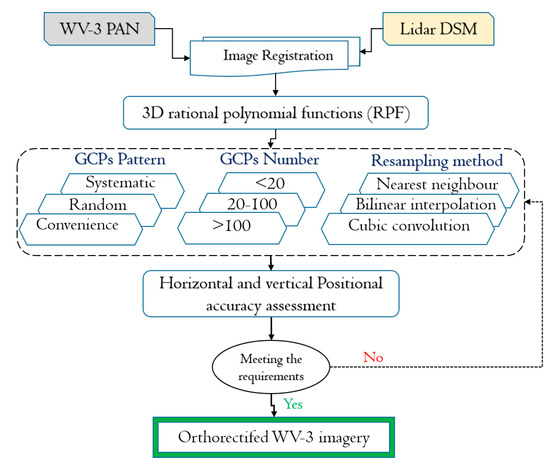
Figure 2.
Overall flowchart of this study.
3.1. Geometric and Registration
The geo-referencing coordinate system of WV-3 PAN images was re-registered with LiDAR airborne dataset based on Malaysian datum (i.e., GDM 2000 MRSO). Two datasets should be completely overlapped before the final orthorectification phase, where the distorting effects of the terrain relief are removed via LiDAR digital surface model (DSM). The software Envi 5.4 was used to process the image.
3.2. Geo-Positioning Model
Geometric sensor models have been generally applied in very-high-resolution (VHR) satellite imagery to discover the relationship between the 3D object positions (X, Y, Z) from the real world, and their corresponding 2D image space positions (x, y) in the map. We assessed multiple experiments on GCP collection and resampling methods for 3D RPC model to orthorectify WV-3 image.
The RPC models are based on the ratios of polynomial equations (see Equations (1) and (2)), where and are the column and row variables in the image, respectively. is the third order polynomial function (Equation (3)) which is also called as 3D rational polynomial function (3D-RPF) [36]., and are three dimensions of the coordinates of any point in object space.
A corresponding transformation based on GCP is vital for completing the orthorectified output. The RPC model is designed from the block adjustment system established by Grodecki and Dial [24] for the image (Equations (4) and (5)).
where are the adjustment factors of the image; and show the differences of the measured line between the measured points for the new set of GCPs in the image space (, ) and the RPCs projected points for the similar GCPs (x, y).
However, only a modest shift is calculated for the zero order of transformation . This shift can be performed by only a single GCP. Once an affine transformation is utilised in the image space, six constants with at least three GCPs must be calculated. However, a third-order 3D rational function model that uses RPCs computes 12 coefficients using minimum six GCPs (Equations (4) and (5)). Table 2 illustrates specification of the RPC model for applied WV-3 imagery.
Table 2.
Rational polynomial coefficients (RPC) specification of WV-3.
In the 3D RPC orthorectification workflow, we implemented geoid correction using the UTM-WGS84 [37] to automatically determine the geoid offset which is displayed in meters. The output pixel size should follow the pixel size of the input datasets which is 0.3 m in our case. The corresponding pixels in the input images through an RPC-based transform can be defined as grid spacing. It ranges from 1 to 10. The RPC orthorectification is faster but less accurate with than without a coarse grid. We selected 1 value as grid spacing because we work with a very high-resolution DSM and satellite image, and the study area has many high-rise buildings.
Engaging bias-corrected RPCs model can result in extremely accurate geo-positioning output which is obviously finer than those attained by older sensors [38].
3.3. Radiometric Methods
The pixel grid of the source image rarely matches that of output orthoimage. Hence, resampling must be performed to assign grey value for the output orthoimage. Resampling can be performed in several ways. The most popular ones are nearest neighbour, bilinear interpolation and cubic convolution (Table 3).
Table 3.
Various types of resampling techniques.
Nearest neighbour (NN) algorithm uses the value of the closest pixel to assign to the output pixel value without any interpolation (Figure 3a), whereas bilinear (BI) algorithm performs a linear interpolation using four pixels to resample the output value (Figure 3b). The cubic convolution (CC) algorithm cubic convolution method engages a window (16 pixels) to compute the output value with a cubic function (Figure 3c).
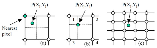
Figure 3.
Techniques of resampling: (a) nearest neighbour (NN), (b) bilinear interpolation (BI) and (c) cubic convolution (CC).
3.4. GCP Quantities and Pattern
Distribution, accuracy and quantity of GCPs are essential metrics for a precise orthorectification system [2]. To achieve a comprehensive assessment, GCPs were selected using random, systematical and convenience selection methods in UTM-WGS84. We classified 220 measured GCPs into three classes—n < 20, 20 < n < 100 and n > 100—to assess the variation of GCP number on the accuracy of orthorectified outputs. Numerous possible GCP numbers are collected via multiple data selection methods to increase the vertical and horizontal accuracies of the output image. Consequently, variances between field-surveyed and corrected image coordinates would be significantly decreased [20,39].
In addition, three well-known patterns for point collection, including random, systematic and convenience, were examined over the study area. The data collection methods applied in this research are listed below:
- Random data collection: The GCPs were collected randomly without any pre-designed strategy.
- Systematic data collection: Firstly, the study area was divided into equal-grid mesh, and then, the GSPs were collected from each grid until the whole image was covered.
- Convenience data collection: The GCPs were collected precisely from well-defined positions, such as corners of buildings (i.e., high-rise built-up that mostly affected by skewness) and edges of swimming pools.
The impact of several contributing parameters on the geometric procedure of the orthorectification phase was investigated in this research as follows: (i) patterns of GCP collection; (ii) number of GCPs involved in the triangulation process ranging from 15 to 220; and (iii) resampling methods. Several combinations of the number of GCPs (n < 20, 20 < n < 100 and n > 100) were generated from the 220 measured GCPs over the study area. Three popular data collection patterns, including random, systematic and convenience patterns, were tested over the study area (i.e., six different GCP combination sets). Three resampling algorithms were then additionally applied on the ideal GCP combinations to discover the highest accurate orthorectified image. All the residual variables were verified for normality of their distribution at Y and X axes. The vertical and horizontal accuracies directly depend on the distribution and the quantity of collected GCPs. A sufficient number of GCPs with regular horizontal and vertical distributions can significantly contribute to the high quality of the orthorectification process [40,41]. Horizontal values can be extracted precisely from a detailed DSM to decrease the uncertainties of RPFs model. The outliers were carefully checked and eliminated from the dataset accordingly. Additionally, the entire extracted coordinates (x, y, z) from LiDAR registration values were normalized in order to conduct the comparison assessment. The RMSE metric was finally applied to verify the accuracy of the corresponding points for any uncertain coordinate. According to the literature, this assessment metric can help ensure the accuracy of the GCP identification on the orthorectified image [32,33].
3.5. Accuracy Assessment
3.5.1. Horizontal Accuracy
Horizontal accuracy can be attained using the horizontal root mean square error () via Equation (6).
where is the root mean square (RMS) difference in eastings between the GCPs and image location in meters; is the RMS difference in northings between the GCP and image location in meters (Equation (7)).
The error X and error Y values for each GCP are the difference in eastings and northings between the GCP and image location in the RPC Refinement. These values can be positive or negative.
The circular standard error (CSE) is another statistical metric for the horizontal accuracy at the 95% confidence level, as shown in Equation (8).
At least 20 GCPs are required for the most accurate CSE value [42]. With one or two GCP adjustments, the RPC model is adjusted by image-space translation.
3.5.2. Vertical Accuracy
The value is calculated using Equation (9). The error Z values for each GCP are reported in the RPC refinement panel [43].
The linear error (LE) metric evaluates the difference between the GCP-measured elevation and the LiDAR DSM elevation with an optional geoid offset in meters at the 95% confidence level using Equation (10).
GCPs with three-time error value of and were considered as outlier points called independent. GCPs were not involved in adjustment processing of the RPC model. GCPs with errors above the threshold shall be recorded as bright white areas.
4. Results
The orthorectification results of this research are discussed in terms of visual distortion and horizontal and vertical errors. The 3D RPC model was assessed according to the number and pattern of GCPS in addition to various resampling algorithms. The GCP points were the height above the ellipsoid. VHR imagery, such as WV-3, needs to be computed via the RPC model. We retrieved GCPs from high-accuracy DSM of LiDAR image with 0.3 spatial resolution (zero offset). With two images captured from the same area, i.e., WV-3 and LiDAR taken from two different viewing angles, parallax effects should be minimised by perfect registration process to refine the RPCs.
RMSEX reflects the lowest error in our rectification process in comparison with other RMSEY, thereby showing the difference between the GCPs and image location in eastings. RMSEY is also low particularly at convenience pattern type because of northing differences between GCPs and the image. Generally, convenience pattern type was an accurate method for collecting GCPs. On top of that, the CC resampling method was the best one in terms of high contract and low uncertainty (Table 4). However, horizontal error is higher than the vertical errors in random and convince data collection methods. A horizontal error is basically due to the difference between the GCPs’ elevation value and corresponding DSM height above the WGS-84 ellipsoid.
Table 4.
Vertical and horizontal accuracy assessments for different patterns of ground control point (GCP) selection with three resampling methods.
Vertical and horizontal accuracies can be improved by selecting a decent pattern of GCP collection [38]. This study proved that the random GCP collection brings high vertical and horizontal errors for orthorectification [16]. The systematic approach slightly improved the accuracy. However, the convenience method, in which the GCPs were collected from buildings’ edges or corners precisely, showed the lowest RMSE error using the 3D RCP model. This improvement is tangible in errors Y and R (Figure 4 and Table 4). However, the resampling algorithms do not significantly contribute to increasing the 3D RCP orthorectification accuracy by considering the variation in resampling algorithm over the applied experiments. In general, the CC method illustrated the best performance in comparison with the two other methods.
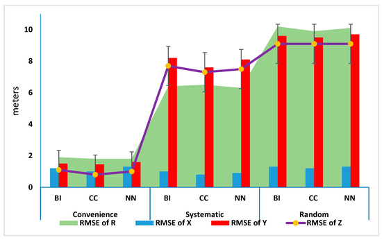
Figure 4.
Horizontal and vertical errors associated with all resampling methods and their GCP collection pattern.
The CSE represented as a horizontal metric and LE computed the vertical error. CSE and LE are subjected to quantity of GCPs. The lowest accuracy was captured once when less than 20 GCPs were involved for orthorectification process. Statistical metrics showed also a significant amount of error when too many GCPs (more than 100) were used as the adjustment GCPs to run the RCP model (Table 5). This result might be due to the negative correlations in between GCPs that should be avoided. However, the best, accurate results in both directions were achieved by engaging 20 to 100 GCPs in our study area. Geoid off set for WV-3 has been constantly −3.03.
Table 5.
Accuracy assessment for different number of GCPs with three resampling methods.
The best scenario of GCP collection and resampling methods for 3D RCP model was observed by applying CC technique and collecting 20 to 100 GCPs with convenience pattern (Figure 5).
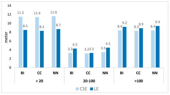
Figure 5.
Variation of circular standard (CSE) and linear error (LE) metrics for different numbers of GCP classes.
The entire area is faced with an error using random selection which causes a wide range of distortion in RCP model. In the other two methods, however, the error distribution was clustered on high-rise buildings. The exact location of oblique buildings was clearly detected by the convenience-based sampling, which can help RCP correct such parts without shifting the geometry of the other parts. Due to the large amount of vertical and horizontal RMSEs for random selection with less than 20 GCPs, these variables were eliminated for the orthorectified visualisation assessment (Figure 6).
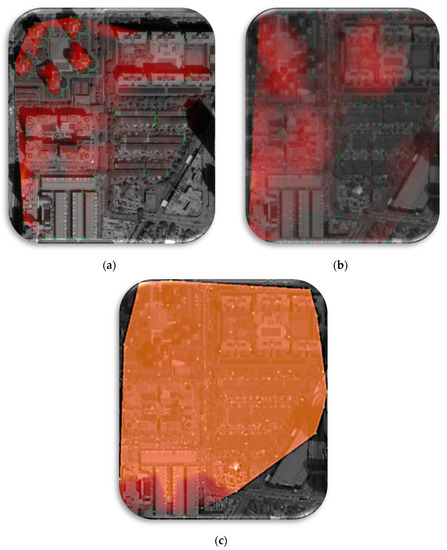
Figure 6.
Error distribution in different GCP collection patterns: (a) convenience, (b) systematic and (c) random.
According to visual interpretation, the amount of distortion is significant when using over-sampling (i.e., more than 100) and systematic sampling of GCPs. In addition, CC method can improve the contrast and smoothness of image in 3D RCP model (Figure 7).
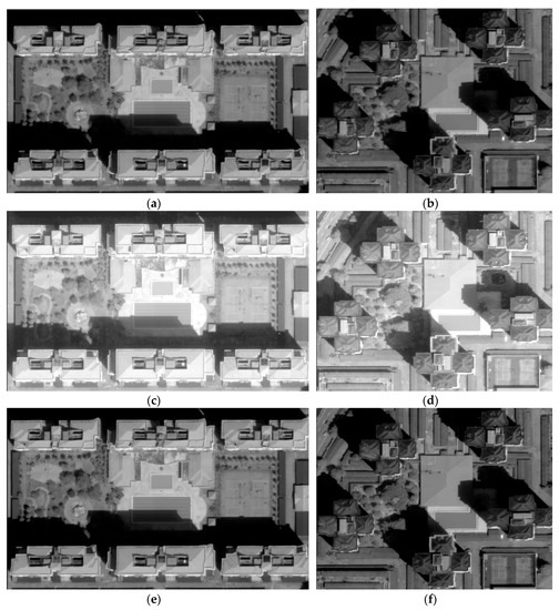
Figure 7.
Comparison of different parametric in 3D RCP model: (a) BI systematic with 80 GCPs over 75 m building, (b) BI systematic with 125 GCPs over 85 m building, (c) CC convenience with 80 GCPs over 75 m building, (d) CC convenience with 120 GCPs over 85 m building, (e) NN systematic with 80 GCPs over 75 m building, (f) NN systematic with 125 GCPs over 75 m building.
Fully parametrised camera models are very sophisticated in applying 0.3 m sensors, such as WV-3 [3]. The 0.3 m LiDAR airborne imagery can be suitable data to be registered with WV-3 to remove the distortion and geometric corrections. In addition, LiDAR DSM is an informative source for collecting precise GCPs for running the RCP orthorectification model.
After extensive experiments on the orthorectification of WV-3 with LiDAR DSM, we found that the 3D RCP model is an accurate approach (Figure 8, Figure 9 and Figure 10). Cubic conventional resampling algorithm offered the finest and smoothest radiometric contrast. In terms of GCP collection, the convenience pattern with 20 to 100 control points achieved the lowest vertical and horizontal uncertainties. The CC algorithm reflected the high contrast of radiometric values. A substantial relationship (R2 = 0.877) exists between the increase or decrease of GCPs’ quantity and RMSE in general (Figure 11).
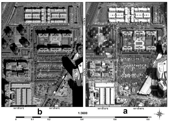
Figure 8.
(a) Original basic WV-3 PAN band and (b) orthorectified image using BI systematic with 80 GCPs.
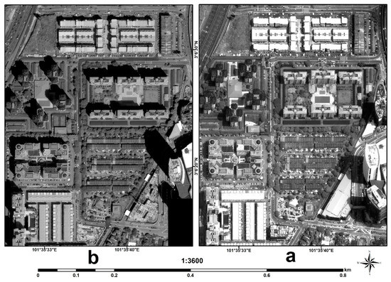
Figure 9.
(a) Original basic WV-3 PAN band and (b) orthorectified image using NN systematic with 80 GCPs.
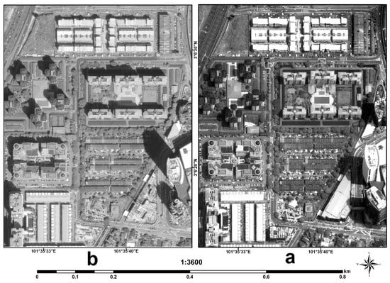
Figure 10.
(a) Original basic WV-3 PAN band and (b) orthorectified image using CC convenience with 80 GCPs.
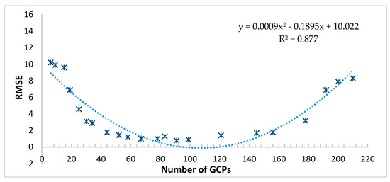
Figure 11.
Exponential regression between number of GCPs and RMSE.
5. Discussions
Detailed and up-to-date land use of the urban environment is required in many applications. A method for applying an accurate orthorectification from VHR satellite images in urban areas, where high-rise buildings generally appear oblique in the image, was presented in this paper. 3D RPC model is considered as a replacement sensor technique for the rigorous sensor with an estimated position of the ground. The accuracy of the 3D RPC depends on the accuracy of GCPs and the original sensor imagery [24]. The 3D RPC is not described as a map projection, but it relates pixel locations in an image to the corresponding longitude, latitude and elevation using a third-order rational polynomial function [44]. In accordance with our experiments, by increasing the number of GCPs from more than 80 to 130, the RMSEs of the outputs remain almost unchanged. However, a further increment than 130 would cause negative effects on accuracy due to spatial overfitting and internal uncoordinated correlation of GCPs on each other. Therefore, it is realized that putting too much effort into collecting more GCPs is not only time consuming but would also possibly decrease the accuracy if it crossed a certain number. Selecting the Convenience approach for GCP collection can result in a more accurate image, since the data collection method is the most significant parameter that contributes to orthorectification processing, rather than the number of GCPs or resampling method. Selecting less than 20 GCPs in even such a small study area produced high error (e.g., more than 4 m). The 20 to 100 GCPs have the lowest error. However, an increment in GCPs did not result in high accuracy. Generally, the orthorectification error would not be reduced necessarily by increasing the GCPs.
The presented experiments show that 3D RPC is a decent method for orthorectification of VHR satellite images. The RPFs require 3D information, i.e., horizontal and vertical coordinates. The result of the proposed model is also precise enough to be integrated with LiDAR data for 3D visualization in details (Figure 12). A sufficient number of GCPs and Convenience GCPs collection method is required to calculate the RPCs precisely. Although horizontal accuracy is lower than vertical accuracies, an accurate DSM extracted from LiDAR can minimise horizontal error substantially. The results showed the considerable effect of LiDAR-DSM on increasing the geometric resolution for the RCP model. Although a stand-alone RPC model is not sufficient for VHR satellite imageries even whilst numerous GCPs are involved, the orthorectification process would be improved if convenience and cubic conventional methods were adopted. Because the 3D RPC correction model is in the form of a fraction, the denominator can be changed dramatically when the GCPs are in the inconvenience distribution and fewer or too many GCPs were involved in RCP training. Therefore, it can cause the morbidity of a standard equation attained by a modelled system that disturbs the stability of 3D RCP model and reduces the accuracy of image orthorectification vertically and horizontally.
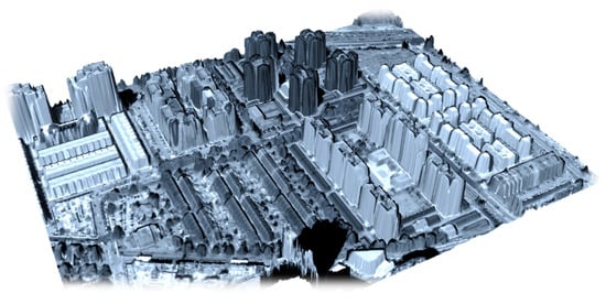
Figure 12.
Orthorectified WV-3 image using 3D RCP model.
6. Conclusions
We successfully orthorectified the VHR satellite image deployed by 3D RCP model. Orthorectified VHR image is required to precisely delineate high-rise buildings from streets and green lands, which is an important process for urban planning. In this research, multiple experiments of generating orthorectified image from WV-3 were assessed to run the 3D RCP model including, number of GCPs, resampling method, and GCPs collection pattern. The accuracy of orthorectified imagery is directly influenced by the horizontal and vertical accuracies of GCPs. GCPs were successfully collected from LiDAR DSM dataset, with high resolution of 0.3 m. After performing different scenarios of resampling and GCP collection in the study area, we discovered that the 3D RCP model delivered the ideal result when 80 GCPs were collected via Convenience pattern. In addition, cubic conventional resampling algorithm made the orthorectified image precise and smooth. We also found out that the data collection method is the most significant parameter rather than the number of GCPs or resampling method. The second important factor, however, was number of GCPs while the least contributing factor to orthorectification accuracy was resampling method. Our proposed combination technique can enhance the vertical accuracy of the geo-positioning process up to 0.8 and 1.8 m for horizontal accuracy (categorised as very-high-accuracy orthorectification procedure) to extract LULC detail mapping in the urban environment. Therefore, it has great potential to be applied in the pre-processing of VHR satellite imagery. Future studies should compare the implemented procedures to other VHR satellite images (e.g., GeoEye-2).
Author Contributions
B.P. conceptualized, designed, collected the data, supervised, and obtained the grant for the study. H.M.R. performed experiments. H.M.R. analyzed the data and wrote the first draft of the manuscript. B.P. contributed to reconstructing, rewriting, and editing the entire paper, including professionally optimizing the manuscript.
Funding
This research is funded by Centre for Advanced Modelling and Geospatial Information Systems, University of Technology Sydney, under Blue-sky grant: 323930, 321740.2232335 and 321740.2232357.
Acknowledgments
The authors would like to express their gratitude to the University of Technology Sydney for providing the Blue-sky funds for this project and supporting remote sensing data analysis and processing.
Conflicts of Interest
The authors declare no conflict of interest.
References
- Zhang, H.; Pu, R.; Liu, X. A new image processing procedure integrating PCI-RPC and ArcGIS-Spline tools to improve the orthorectification accuracy of high-resolution satellite imagery. Remote Sens. 2016, 8, 827. [Google Scholar] [CrossRef]
- Piero, B.; Borgogno Mondino, E.; Tonolo, F.G.; Andrea, L. Orthorectification of high resolution satellite images. Int. Arch. Photogramm. Remote Sens. Spat. Inf. Sci. 2004, 35, 30–35. [Google Scholar]
- Mojaddadi Rizeei, H.; Pradhan, B.; Saharkhiz, M.A. Urban object extraction using Dempster Shafer feature-based image analysis from worldview-3 satellite imagery. Int. J. Remote Sens. 2019, 40, 1092–1119. [Google Scholar] [CrossRef]
- Rizeei, H.M.; Shafri, H.Z.; Mohamoud, M.A.; Pradhan, B.; Kalantar, B. Oil palm counting and age estimation from WorldView-3 imagery and LiDAR data using an integrated OBIA height model and regression analysis. J. Sens. 2018, 2018. [Google Scholar] [CrossRef]
- Aal-shamkhi, A.D.S.; Mojaddadi, H.; Pradhan, B.; Abdullahi, S. Extraction and modeling of urban sprawl development in Karbala City using VHR satellite imagery. In Spatial Modeling and Assessment of Urban Form; Springer: Berlin/Heidelberg, Germany, 2017; pp. 281–296. [Google Scholar]
- Abdullahi, S.; Pradhan, B.; Mojaddadi, H. City compactness: Assessing the influence of the growth of residential land use. J. Urban Technol. 2018, 25, 21–46. [Google Scholar] [CrossRef]
- Mojaddadi, H.; Pradhan, B.; Nampak, H.; Ahmad, N.; Ghazali, A.H.B. Ensemble machine-learning-based geospatial approach for flood risk assessment using multi-sensor remote-sensing data and GIS. Geomat. Nat. Hazards Risk 2017, 8, 1080–1102. [Google Scholar] [CrossRef]
- Nampak, H.; Pradhan, B.; Mojaddadi Rizeei, H.; Park, H.J. Assessment of land cover and land use change impact on soil loss in a tropical catchment by using multitemporal SPOT-5 satellite images and R evised U niversal Soil L oss E quation model. Land Degrad. Dev. 2018, 29, 3440–3455. [Google Scholar] [CrossRef]
- Rizeei, H.M.; Pradhan, B.; Saharkhiz, M.A. Surface runoff prediction regarding LULC and climate dynamics using coupled LTM, optimized ARIMA, and GIS-based SCS-CN models in tropical region. Arab. J. Geosci. 2018, 11, 53. [Google Scholar] [CrossRef]
- Rizeei, H.M.; Saharkhiz, M.A.; Pradhan, B.; Ahmad, N. Soil erosion prediction based on land cover dynamics at the Semenyih watershed in Malaysia using LTM and USLE models. Geocarto Int. 2016, 31, 1158–1177. [Google Scholar] [CrossRef]
- Leprince, S.; Barbot, S.; Ayoub, F.; Avouac, J.-P. Automatic and precise orthorectification, coregistration, and subpixel correlation of satellite images, application to ground deformation measurements. IEEE Trans. Geosci. Remote Sens. 2007, 45, 1529–1558. [Google Scholar] [CrossRef]
- Chmiel, J.; Kay, S.; Spruyt, P. Orthorectification and geometric quality assessment of very high spatial resolution satellite imagery for Common Agricultural Policy purposes. In Proceedings of the XXth ISPRS Congress, Istanbul, Turkey, 12–23 July 2004; pp. 12–23. [Google Scholar]
- Mezaal, M.; Pradhan, B.; Rizeei, H. Improving Landslide Detection from Airborne Laser Scanning Data Using Optimized Dempster–Shafer. Remote Sens. 2018, 10, 1029. [Google Scholar] [CrossRef]
- Rizeei, H.M.; Azeez, O.S.; Pradhan, B.; Khamees, H.H. Assessment of groundwater nitrate contamination hazard in a semi-arid region by using integrated parametric IPNOA and data-driven logistic regression models. Environ. Monit. Assess. 2018, 190, 633. [Google Scholar] [CrossRef] [PubMed]
- Dowman, I.; Dare, P. Automated procedures for multisensor registration and orthorectification of satellite images. In Proceedings of the International Archives of Photogrammetry and Remote Sensing, Valladolid, Spain, 3–4 June 1999. [Google Scholar]
- Marsetič, A.; Oštir, K.; Fras, M.K. Automatic orthorectification of high-resolution optical satellite images using vector roads. IEEE Trans. Geosci. Remote Sens. 2015, 53, 6035–6047. [Google Scholar] [CrossRef]
- Chen, L.-C.; Teo, T.-A.; Rau, J.-Y. Optimized patch backprojection in orthorectification for high resolution satellite images. Int. Arch. Photogramm. Remote Sens 2004, 35, 586–591. [Google Scholar]
- Fraser, C.S.; Dial, G.; Grodecki, J. Sensor orientation via RPCs. ISPRS J. Photogramm. Remote Sens. 2006, 60, 182–194. [Google Scholar] [CrossRef]
- Aguilar, M.A.; del Mar Saldana, M.; Aguilar, F.J. Assessing geometric accuracy of the orthorectification process from GeoEye-1 and WorldView-2 panchromatic images. Int. J. Appl. Earth Obs. Geoinf. 2013, 21, 427–435. [Google Scholar] [CrossRef]
- Toutin, T. Geometric processing of remote sensing images: Models, algorithms and methods. Int. J. Remote Sens. 2004, 25, 1893–1924. [Google Scholar] [CrossRef]
- Fraser, C.S.; Hanley, H.B. Bias-compensated RPCs for sensor orientation of high-resolution satellite imagery. Photogramm. Eng. Remote Sens. 2005, 71, 909–915. [Google Scholar] [CrossRef]
- Crespi, M.; Fratarcangeli, F.; Giannone, F.; Pieralice, F. High resolution satellite image orientation models. In Geospatial Technology for Earth Observation; Springer: Berlin/Heidelberg, Germany, 2010; pp. 63–104. [Google Scholar]
- Erdogan, M.; Yilmaz, A.; Eker, O. The georeferencing of RASAT satellite imagery and some practical approaches to increase the georeferencing accuracy. Geocarto Int. 2016, 31, 647–660. [Google Scholar] [CrossRef]
- Grodecki, J.; Dial, G. Block adjustment of high-resolution satellite images described by rational polynomials. Photogramm. Eng. Remote Sens. 2003, 69, 59–68. [Google Scholar] [CrossRef]
- Zoej, M.V.; Mokhtarzade, M.; Mansourian, A.; Ebadi, H.; Sadeghian, S. Rational function optimization using genetic algorithms. Int. J. Appl. Earth Obs. Geoinf. 2007, 9, 403–413. [Google Scholar] [CrossRef]
- Toutin, T. Three-Dimensional Geometric Correction of Earth Observation Satellite Data. In Advances in Environmental Remote Sensing; CRC Press: Boca Raton, FL, USA, 2011; pp. 173–217. [Google Scholar]
- Ono, T.; Hattori, S.; Hasegawa, H.; Akamatsu, S.-i. Digital mapping using high resolution satellite imagery based on 2D affine projection model. Int. Arch. Photogramm. Remote Sens. 2000, 33, 672–677. [Google Scholar]
- Singh, M.K.; Gupta, R.; Snehmani; Bhardwaj, A.; Ganju, A. Effect of sensor modelling methods on computation of 3-D coordinates from Cartosat-1 stereo data. Geocarto Int. 2016, 31, 506–526. [Google Scholar] [CrossRef]
- Poli, D.; Toutin, T. Review of developments in geometric modelling for high resolution satellite pushbroom sensors. Photogramm. Rec. 2012, 27, 58–73. [Google Scholar] [CrossRef]
- Cheng, P.; Toutin, T. Ortho Rectification and DEM generation from high resolution satellite data. In Proceedings of the 22nd Asian Conference on Remote Sensing, Singapore, 5–9 November 2001; p. 9. [Google Scholar]
- Qin, Z.; Li, W.; Li, M.; Chen, Z.; Zhou, G. A methodology for true orthorectification of large-scale urban aerial images and automatic detection of building occlusions using digital surface model. In Proceedings of the Geoscience and Remote Sensing Symposium, Toulouse, France, 21–25 July 2003; pp. 729–731. [Google Scholar]
- Wolniewicz, W. Assessment of geometric accuracy of VHR satellite images. Proceeding Xxth Int. Arch. Photogramm. Remote Sens. Spat. Inf. Sci. 2004, 35, 12–23. [Google Scholar]
- Afify, H.; Zhang, Y. Accuracy Assessment of User-Derived RFCs for Ortho-Rectification of High-Resolution Satellite Imagery. Int. J. Geoinform. 2008, 4, 17–24. [Google Scholar]
- Maglione, P.; Parente, C.; Vallario, A. Using rational polynomial functions for rectification of GeoEye-1 imagery. IOSR J. Appl. Geol. Geophys. 2013, 1, 12–17. [Google Scholar] [CrossRef]
- Capaldo, P.; Crespi, M.; Fratarcangeli, F.; Nascetti, A.; Pieralice, F. DSM generation from high resolution imagery: Applications with WorldView-1 and Geoeye-1. Ital. J. Remote Sens. 2012, 44, 41–53. [Google Scholar] [CrossRef]
- Tao, C.V.; Hu, Y. A comprehensive study of the rational function model for photogrammetric processing. Photogramm. Eng. Remote Sens. 2001, 67, 1347–1358. [Google Scholar]
- Pavlis, N.K.; Holmes, S.A.; Kenyon, S.C.; Factor, J.K. The development and evaluation of the Earth Gravitational Model 2008 (EGM2008). J. Geophys. Res. Solid Earth 2012, 117. [Google Scholar] [CrossRef]
- Fraser, C.; Ravanbakhsh, M. Georeferencing performance of GEOEYE-1. Photogramm. Eng. Remote Sens. 2009, 75, 634–638. [Google Scholar]
- Raabe, E.A.; Stumpf, R.P. Image Processing Methods; Procedures in Selection, Registration, Normalization and Enhancement of Satellite Imagery in Coastal Wetlands; US Geological Survey, Center for Coastal Geology: St. Petersburg, FL, USA, 1997.
- Errico, A.; Guastaferro, F.; Parente, C.; Santamaria, R. Applications on geometric correction of different resolution satellite images. In Proceedings of the IEEE GOLD Conference 2010, Livorno, Italy, 29–30 April 2010. [Google Scholar]
- Guastaferro, F.; Maglione, P.; Parente, C. Rectification of spot 5 satellite imagery for marine geographic information systems. In Proceedings of the Advanced Research in Scientific Areas Virtual International Conference, Žilina, Slovakia, 3–7 December 2012; pp. 3–7. [Google Scholar]
- Authority, T.V. Geospatial Positionng Accuracy Standards Part 3: National Standard for Spatial Data Accuracy; National Aeronautics and Space Administration: Virginia, NV, USA, 1998.
- Kapnias, D.; Milenov, P.; Kay, S. Guidelines for Best Practice and Quality Checking of Ortho Imagery; Joint Research Centre: Ispra (VA), Italy, 2008. [Google Scholar]
- McGlone, J. Manual of Photogrammetry, 5th ed.; The American Society for Photogrammetry and Remote Sensing: Bethesda, MD, USA, 2004. [Google Scholar]
© 2019 by the authors. Licensee MDPI, Basel, Switzerland. This article is an open access article distributed under the terms and conditions of the Creative Commons Attribution (CC BY) license (http://creativecommons.org/licenses/by/4.0/).