Article

Continuous Monitoring of Cotton Stem Water Potential using Sentinel-2 Imagery

1
Department of Geosciences, Texas Tech University, Lubbock, TX 79409, USA
2
Aerospace Information Research Institute, Chinese Academy of Sciences, Beijing 100094, China
3
Department, University of Chinese Academy of Sciences, Beijing 100049, China
4
Department of Natural Resources and the Environment, University of Connecticut, Storrs, CT 06269, USA
5
Department of Plant and Soil Science, Texas Tech University, Lubbock, TX 79409, USA
6
Department of Soil and Crop Sciences, Texas A&M AgriLife Research, Lubbock, TX 79403, USA
7
The Climate Corporation, San Francisco, CA 94103, USA
8
The Climate Corporation, Saint Louis, MO 63141, USA
*
Author to whom correspondence should be addressed.
Remote Sens. 2020, 12(7), 1176; https://doi.org/10.3390/rs12071176
Submission received: 19 February 2020 / Revised: 27 March 2020 / Accepted: 2 April 2020 / Published: 6 April 2020
(This article belongs to the Special Issue Smart Farming and Land Management Enabled by Remotely Sensed Big Data)

Abstract

:
Monitoring cotton status during the growing season is critical in increasing production efficiency. The water status in cotton is a key factor for yield and cotton quality. Stem water potential (SWP) is a precise indicator for assessing cotton water status. Satellite remote sensing is an effective approach for monitoring cotton growth at a large scale. The aim of this study is to estimate cotton water stress at a high temporal frequency and at a large scale. In this study, we measured midday SWP samples according to the acquisition dates of Sentinel-2 images and used them to build linear-regression-based and machine-learning-based models to estimate cotton water stress during the growing season (June to August, 2018). For the linear-regression-based method, we estimated SWP based on different Sentinel-2 spectral bands and vegetation indices, where the normalized difference index 45 (NDI45) achieved the best performance (R2 = 0.6269; RMSE = 3.6802 (-1*swp (bars))). For the machine-learning-based method, we used random forest regression to estimate SWP and received even better results (R2 = 0.6709; RMSE = 3.3742 (-1*swp (bars))). To find the best selection of input variables for the machine-learning-based approach, we tried three different data input datasets, including (1) 9 original spectral bands (e.g., blue, green, red, red edge, near infrared (NIR), and shortwave infrared (SWIR)), (2) 21 vegetation indices, and (3) a combination of original Sentinel-2 spectral bands and vegetation indices. The highest accuracy was achieved when only the original spectral bands were used. We also found the SWIR and red edge band were the most important spectral bands, and the vegetation indices based on red edge and NIR bands were particularly helpful. Finally, we applied the best approach for the linear-regression-based and the machine-learning-based methods to generate cotton water potential maps at a large scale and high temporal frequency. Results suggests that the methods developed here has the potential for continuous monitoring of SWP at large scales and the machine-learning-based method is preferred.

Graphical Abstract

1. Introduction

The decrease of regional precipitation and the increase in evapotranspiration driven by climate change will result in increasing drought in the near future [1,2,3,4]. More intense and longer droughts have devastating impacts on the environment [3]. For agriculture, drought can endanger food security which can have critical effects on the economy, geopolitics, and society [5]. Drought can also negatively affect agriculture production especially in arid and semiarid regions [6]. Therefore, detecting crop water stress is of vital importance to improve agricultural quality and productivity.
Cotton is cultivated in arid and semiarid regions and is the most important fiber crop in the world [7]. Cotton is susceptible to water stress in all growth stages, particularly during the flowering and boll development stages [8]. Moreover, water deficit is an important factor limiting growth and development in cotton, including plant height, leaf and root size, as well as economic yield and fiber quality [8]. To better understand the cotton’s response and adaption to water stress, continuous monitoring of cotton water status in large areas would be essential [9].
Traditional methods for water stress assessment rely on measuring temperature [10], physiological response [11] and soil moisture [12]. The crop water stress index (CWSI) is calculated by canopy temperature and has been widely used to quantify crop water stress [13,14], though different dates may show different correlations [15]. The modified crop water stress index (MCWSI) has mitigated the problem of temporal variability [16]. The comprehensive stress indicator (CSI), which is based on leaf temperature and relative humidity, is also useful for water status assessing [17]. However, these approaches are unsuitable for farmers to adopt due to the difficulty in making them fully automated and operational.
Recently, some studies have explored the use of vegetation indices (VIs) for automated monitoring of crop water status and optimizing irrigation schedule at the canopy and landscape scales [18,19,20,21,22,23]. These physical-based approaches have been used to estimate crop water status at the field scale for wheat [20], cotton [24], maize [25], and vineyard [26,27] These approaches can effectively avoid irreversible damage and yield loss in the estimation of crop water status. However, the response to water stress is crop specific and varies for different kinds of vegetation indices. It is still unknown which kinds of vegetation indices have the best performance on cotton water stress.
Though the physical-based approaches can provide direct insights on the relationship between the satellite observation and the response to water stress, they rely heavily on the predefined assumption of the relationship, such as a linear model. Moreover, the physical-based approaches usually can only take one or a few variables as inputs for their models and will be overwhelmed easily given the high dimensions of satellite data, particularly when the physical relationship is nonlinear. Therefore, more advanced machine learning methods, such as neural networks and random forest, are being used widely for estimating physical parameters when there are sufficient training data available [28,29]. Therefore, it is interesting to explore how well we can use a machine-learning-based approach (it is better than physical-based approach or worse?), such as random forest, for estimating crop water stress, and which combinations of variables can provide the best results.
Remote sensed imagery has long been recognized as a direct measure of plant water stress estimation [30,31,32]. Infrared thermal imaging collected by Landsat or MODIS (onboard Terra and Aqua) offers the potential of acquiring the surface temperature from which the water potential can be estimated [33,34]. It remains difficult, however, to collect high spatial resolution thermal remotely sensed imagery. Though water status monitoring with WorldView-2 is achievable [35], the commercial satellite has limitations in large area applications due to the high cost and small swath size [36]. Unlike space-borne satellites, handheld spectroradiometer and unmanned aerial vehicle (UAV) allows for local mapping at higher spatial and temporal resolutions. Moreover, they can monitor plant water status and aid irrigation water management [30,37,38]. Due to handheld spectroradiometer’s limited range and UAVs’ limited flight time, they require more measurements to cover a large area [25,39]. Therefore, it is important to have a system that is capable for monitoring crop water status fully automated and providing non-destructive, continuous estimates.
The Sentinel-2 satellites are potentially useful in crop water stress estimation due to its rich spectral information. The twin satellites with 10-20-60 m spatial resolution and five-day revisit frequency also provides a valuable open data resource for on-the-ground crop management for farmers. The effectiveness of using Sentinel-2 imagery for the detection of water stress on grapevines has been demonstrated [40]. Although spectral indices have relatively significant relationships with physiological measurements, the use of a single vegetation index for predicting crop water status may not be optimal. Innovative approaches based on machine learning and multiple spectral dimensions could be beneficial [38].
The goal of this study is to develop an algorithm for continuous monitoring of cotton water stress at a large scale by using Sentinel-2 images. The word “continuous” here means the method can produce the map of cotton water stress as soon as newly collected images are available in a continuous mode. Two different approaches were compared to estimate cotton water stress: the linear-regression-based and the machine-learning-based approaches. In the linear-regression-based approach, we developed an empirical relationship between different Sentinel-2 spectral bands/vegetation indices and the ground measured cotton water stress values using a linear-regression-based approach. In the machine-learning-based approach, we employed random forest model to estimate SWP due to its high non-linear regression precision and its wide applicability [41]. Three different input strategies (9 original spectral bands, 21 vegetation indices, and a combination of original spectral bands and vegetation indices) were compared in the study.

2. Materials and Methods
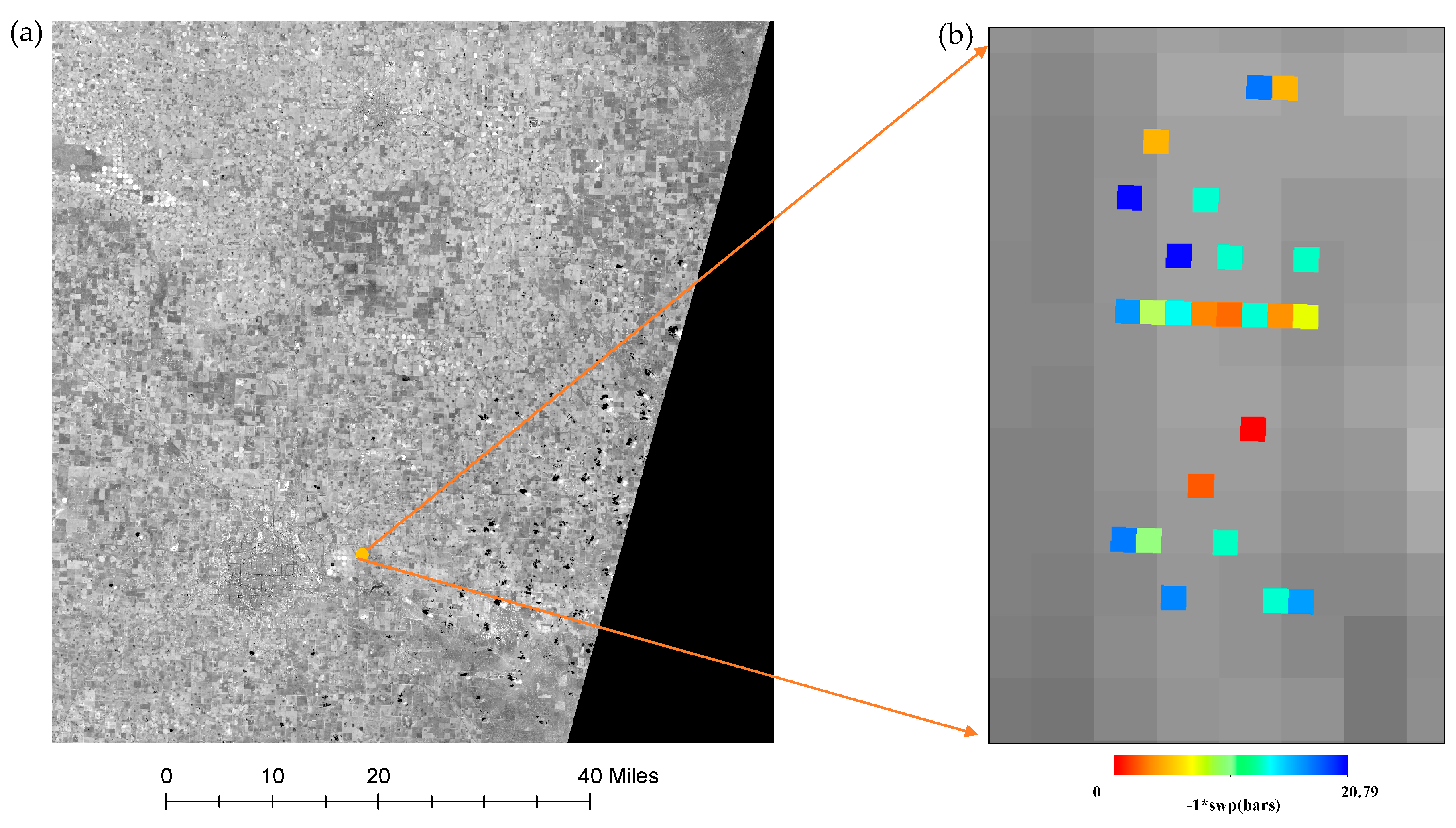
2.1. Study Area

This study was conducted on a research farm planted with cotton in the Southern High Plains of Texas in 2018. The state of Texas accounts for approximately 50% of US cotton production [42]. Water is the key limiting factor in crop production in the Texas High Plains. It has a semi-arid climate with annual precipitation of approximately 500mm and high evaporation demand. Low precipitation and heavy irrigation have resulted in a steady decline in water supply in Lubbock, Texas (Figure 1a). Producers with irrigated cotton are challenged to maintain production with diminishing water resource and the harsh climatic environment. The soil type of the study area is loam. Figure 1b shows the experiment in the paper consisted of 8 zones and 26 ranges of plots, and the 24 labeled plots with cyan squares are the measured SWP. All the plots in the experiment consisted of four irrigation rates which are 100%, 25%, 50%, 75%, 50%, 75%, 25% and 100%, respectively, from the left to the right zones. Each plot had an 8.1 m width and 7.6 m length and contained eight rows of cotton. The irrigation treatment was implemented using a subsurface drip irrigation system. Different rates of irrigation were started on June 18, 2018, and ended on September 6, 2018. The irrigation amount changed weekly on Monday. An ATMOS 41 weather station (METER Group, Pullman, WA) was installed in the field for recording weather data. The precipitation was measured from January 1, 2018 to November 11, 2018 in the cotton field. The precipitation value ranged from 0 to 0.54 inches with an average value of 0.039 inches during the cotton growing season (Figure 2). The weekly irrigation amount was derived by using the actual crop evapotranspiration (ETc) minus the effective rainfall of the previous week.

2.2. Reference Data

Effective measurement of plant leaf water status provides information about plant water stress conditions. We measured five main cotton growing stages: (1) germination and emergence (June 15, 2018), (2) seedling establishment (June 29, 2018), (3) leaf area and canopy development (July 11, 2018), (4) flowering and boll development (August 1, 2018), and (5) maturation (August 23, 2018). In this study, midday stem water potential was measured as an effective water stress indicator for identifying the plants in moderate or severe water deficits [43]. Midday stem water potential was determined by leaves that were in good condition and enclosed in aluminum foil bags for at least 15 minutes to prevent transpiration. In each experimental plot, three healthy leaves were sampled aiming for the mid-value to represent the water potential of the corresponding plot. The statistical range of measured SWP values was illustrated in Figure 3. The average SWP shows a gradual increase during the growing season. The overall average SWP was 15.31 (-1*swp (bars)) with a standard deviation of 5.89 (-1*swp (bars)), a minimum value of 2.55 (-1*swp (bars)) and a maximum value of 27.13 (-1*swp (bars)). The SWP was measured once a week from the beginning of the irrigation season until the boll stage using a pressure chamber. The amount of pressure indicates how much tension the leaf was experiencing on its water: a high value of pressure meant a high value of tension and a high degree of water stress. The unit of pressure is bars and 1 bar equals to 1 atmosphere of pressure.

2.3. Pre-processing

The Sentinel-2 twin satellites can provide various information on vegetation, soil, inland river and coastal environment [44,45,46]. The twin satellites are in the same orbit, phased at 180° to each other. The first satellite, Sentinel-2A, was launched on June 23, 2015 and the second satellite, Sentinel-2B was launched on March 7, 2017. The twin satellites with a height of 785 km and a swath width of 290 km carry a single multi-spectral instrument (MSI) each which covers 13 spectral bands. The spatial resolution of MSI is 10 m (three visible spectral bands and a narrow NIR spectral band), 20 m (three red edge spectral bands, a NIR spectral band and two SWIR spectral bands) and 60m (a Coastal aerosol spectral band, a water vapor spectral band and a cirrus spectral band) respectively [47] (Table 1). We used bands 2–7, band 8A and bands 11–12 for linear regression, and random forest regression in this study (Table 1). As the narrower infrared channel could improve the quality of the vegetation index, it was used in calculating vegetation indices [48]. We selected five relatively cloudless Sentinel-2 images with dates of 06/15/2018 (Sentinel-2B), 06/27/2018 (Sentinel-2A), 07/10/2018 (Sentinel-2A), 08/01/2018 (Sentinel-2B), and 08/24/2018 (Sentinel-2B) to analyze SWP during the cotton growing season in this study. The images were atmospherically corrected and resampled to 20 m (based on nearest neighborhood method) using the sen2cor plugin, which can be installed and run directly in SeNtinel Application Platform (SNAP) software [49]. The cloud and cloud shadow masks were derived from the Fmask4.0 algorithm [50].
Figure 4 shows the entire study area of Sentinel-2 (Figure 4a) and the measured SWP overlay on a small subset of Sentinel-2 image (Figure 4b). Though the ground measured SWP and Sentinel-2 images were geo-corrected and linked to each other, there is still geometric differences between the target plot and Sentinel-2 images (Figure 4b). The size of each plot is 8.1 m in width and 7.6 m in length and the spatial resolution of Sentinel-2 image is 20 m. The measured SWP ranged from 2.55 (-1*swp (bars)) to 20.79 (-1*swp (bars)) with dates of June 15, 2018 in the target plots. The number of pixels occupied by the entire study area in Sentinel-2 was 52. We calculated the area weighted average of ground measured SWP to represent the SWP within the Sentinel-2 pixel [51].

2.4. Linear-Regression-Based Method

The least squares linear regression between the vegetation indices and stem water potential were obtained in this study. We tested 9 spectral bands and 21 Vegetation Indices (VIs) to establish a linear relationship with SWP during the growing season (Table 2). The indices using visible and near-infrared bands were developed to predict crop water stress due to their positive correlations with stomatal conductance and leaf water potential [22,23]. Many studies have suggested that these indices are nearly linear related to stem water potential [24,31,52,53]. The red edge-based vegetation indices were also compared in the study, due to their sensitive to chlorophyll content and leaf area index (LAI) [54,55]. Moreover, the water absorption bands in the 1300–2500 nm region, which can eliminate variations caused by leaf internal structure and leaf dry matter content, are most sensitive to the leaf water content of most crops [56]. The indices created by the combination of the NIR and the SWIR bands can substantially improve the accuracy of retrieving the vegetation water content [57], which were widely used to monitor changes in stem water potential in the literature [24,25,58].

2.5. Machine-Learning-Based Method

The non-linear random forest (RF) regression method was also examined to predict the cotton stem water potential. RF is a robust, supervised machine learning algorithm used for classification and regression [75]. It is the integration of a multitude of unpruned tress which are trained by bagging (i.e., bootstrap aggregation) [76]. The bagging uses the randomly selected training data and then constructs the classifier. Three datasets were evaluated as input into the RF regression algorithm: (1) spectral bands of Sentinel-2 imagery, (2) 21 vegetation indices, and (3) spectral bands combined with spectral indices. We used the TreeBagger function in MATLAB and the parameter “ntree” was set as 100. The parameter “mtry” was set as the default for all the three input strategies of RF. The total number of training and testing pixels was 52, in which 80% of the data were randomly selected as training samples, and the remaining 20% were used as validation.

3. Results

3.1. Linear-Regression-Based Approach

We conducted 30 experiments to test the effective linear relationship between original spectral bands of Sentinel-2, different spectral index, and the ground measured cotton stem water stress values (Figure 5). The R square values calculated from all reference samples (n = 52) were used to evaluate the performance of different linear-regression-based methods. The high R square values (R square > 0.5) represented strong correlation between spectral features and SWP [35]. Figure 5 showed that most of these models had a relatively strong correlation over time. The vegetation index of NDI45 had the best linear relationship with cotton water potential. NDI45, MCARI, and GNDVI were the three best-performed models, which were calculated by the green, red and red edge bands. For a single spectral band, its correlation with stem water potential was relatively lower than VIs. The red and SWIR bands showed a better linear relationship with the stem water potential compared to other spectral bands. For the start of the season (June 15, 2018), the field just started to grow, and the vegetation is sparse. Therefore, due to the different irrigation level in the field, the blue dots in Figure 5 varied a lot in SWP. For the middle of the season (June 29, 2018-August 1, 2018), the leaf area and the boll has developed. The cyan, green and yellow dots showed a strong linear correlation between spectral features and SWP. For the end of the season (August 23, 2018), the cotton was at the early-maturing stage and the SWP reached to their maximum.

3.2. Machine-Learning-Based Approach

We also used random forest regression to establish the relationship between Sentinel-2 data and stem water potential, and three scenarios (original bands, vegetation indices, and the combined use of the two) were compared. Considering the machine-learning-based approach may subject to overfitting, we compared algorithm performance based on a five-fold cross-validation approach, in which 80% of the data were randomly selected as training, and the remaining 20% were used to calculate R square and RMSE (Table 3). Surprisingly, the use of just the surface reflectance bands from Sentinel-2 has the highest R square and lowest RMSE. The vegetation indices alone and the combined use of spectral bands and vegetation indices all showed lower accuracies. We think it is mainly because the vegetation indices are derived from the spectral bands and if a good machine learning approach is used, such as random forest, all the information contained within the spectral bands has already been well-learned, and the use of extra derivation from the spectral bands (e.g., vegetation indices) would only have negative impact by increasing data dimension, instead of brining any extra information. Figure 6 shows the scatterplot of best-performed random forest estimated (based on original bands) and measured SWP for all 52 reference samples. We can see that the random forest estimated values are very close to the actual measurements.

3.3. Comparing Best Approaches from Linear-Regression-Based and maching-Learning-Based Methods

For cotton, SWP varied with growing stage. As such, non-linear machine-learning-based method, which included more input variables, can better explain variability in cotton water stress. To better compare the best approaches from linear-regression-based method (based on NDI45) and the machine-learning-based method (based on original surface reflectance bands), we calculated RMSE and R square for the linear-regression-based method (based on NDI45) following the same five-fold cross-validation approach. The best approach from the machine-learning-based method achieved a much higher R square (0.6709) and lower RMSE (3.3742) than the best approach from the linear-regression-based method (R square = 0.6157 and RMSE = 3.6802). This suggests that though the linear-regression-based method is relatively simple and easy to use, the machine-learning-based method can provide more accurate detection of SWP due to its capability of including high dimensions of data. This was further emphasized that single VI was not sensitive enough to SWP, so that additional spectral features on SWP estimation was of significance.

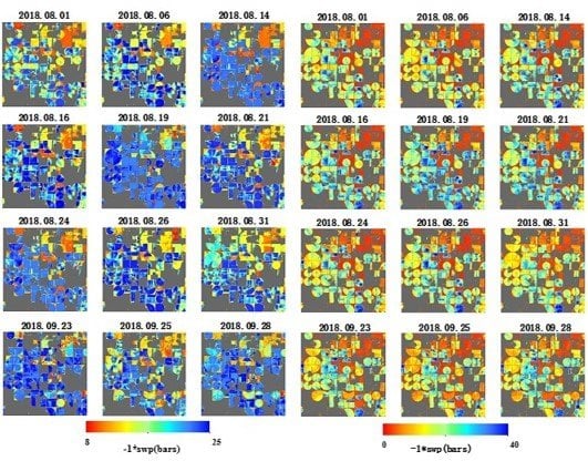
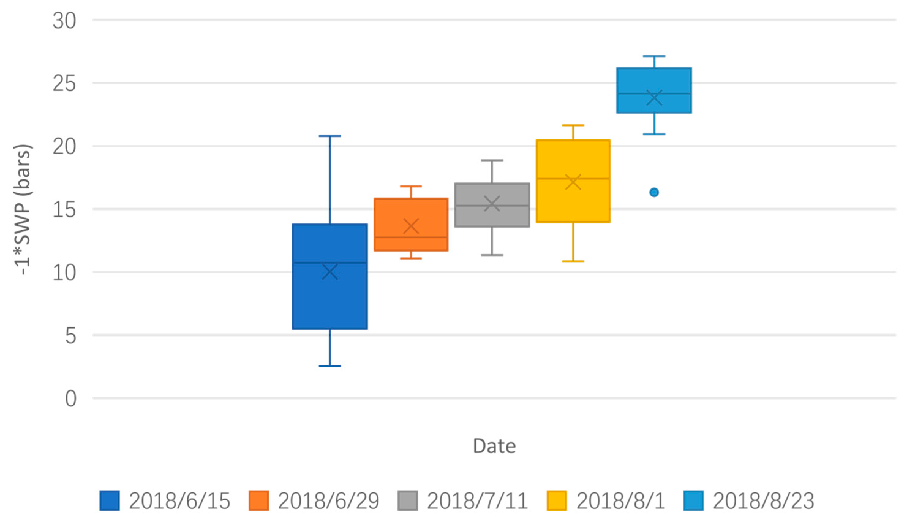
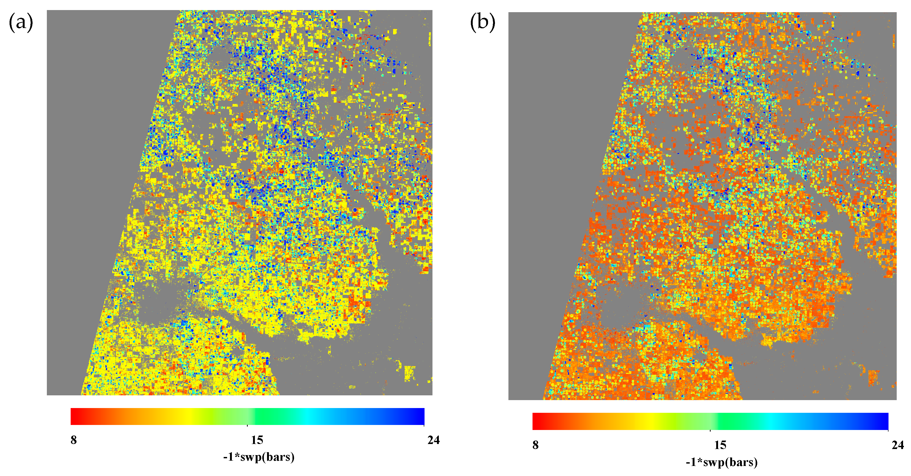
3.4. Comparing Results Spatially and Temporally

We explored the potential of using this approach to continuous monitoring of the stem water potential of cotton at a large scale. Images of the stem water potential maps for Sentinel-2 based on random forest regression method and the linear regression method are shown in Figure 7. The map of Figure 7a was derived from random forest regression when all the original surface reflectance bands of Sentinel-2 were used as the input. The map of Figure 7b was derived from the best performed linear regression method (NDI45). The cotton mask was derived from Crop Data Layer 2018 (CDL) [77]. A visual comparison of random forest regression and linear regression shows the random forest regression model estimates are higher than the linear regression approach does. However, the estimation of the two regression approaches are consistent at the region with a high level of stem water potential. Note that this is mainly for qualitative comparison and considering the massive amount of work to collect field data of stem water potential of cotton at a large scale over time, we did not provide any quantitative metrics to provide the error analysis for the maps generated below.
By applying the same technique for time series of Sentinel-2 images, we can monitor water potential continuously (Figure 8). Figure 8 shows the spatial distribution of SWP changes in the sample scene of cotton field during the growing season. In the sample scene, there was an obvious ascend trend of SWP within August 1–21, and a descend trend within August 28 to September 21 for machine-learning-based estimation. For linear-regression-based estimation, the SWP had no obvious change.
The histogram of stem water potential from Figure 7 maps was computed and shown in Figure 9. The largest stem water potential ranged from 9 to 10.5 in the linear-regression-based method and ranged from 13.5 to 15 in the random forest regression method. For the linear regression method, the estimated stem water potential values were sometimes outside the normal range including negative values. For the machine-learning-based method, however, the estimated stem water potential values were in the normal range and were closer to the measured value according to RMSE.
The two-year estimates of stem water potential for one pixel is illustrated in Figure 10. The time series plot of estimated water potential results from the best linear regression method and the best random forest regression method were compared. For the linear regression time series result, the value of stem water potential was relatively stable at the beginning of the cotton growing stage and then rose rapidly at the flowering stage. As for the random forest regression result, the curve was not stable but represented a rising trend generally.

4. Discussion

The cotton water demand is different at different stages of cotton growth and development [78]. Moreover, the spectral features of water indices reflected water stress to a certain extent [24]. Due to the self-regulation mechanism of crop, the sensitivity of crop to water stress are reflected on its growth and development [79]. The linear regression result illustrated that though the irrigation level was different at the early stage of planting, the SWP value of cotton was almost the same for the mature stage. For precise irrigation, water use was relatively low at this cotton planting stage. It can be seen from the strong linear relationship between spectral features and SWP, in which water was critical from the germination to flowering stage. Once the bolls started to open, the irrigation level of cotton should be allowed to reduce for better harvest conditions. Compared with linear-regression-based method, the machine-learning-based method performed better in SWP estimation based on accuracy metrics such as R square and RMSE. This will possibly be a small but positive step towards continuous irrigation scheduling for efficient growth-stage-specific water application in cotton.
Our linear regression results showed that most VIs are suitable predictors for cotton stem water potential. The VIs based on the red and red edge spectral bands (NDI45, MCARI) were the best candidates as they are more sensitive to stomatal conductance and leaf water potential [58]. The positive correlation between the NDI45 or MCARI, and SWP showed these VIs is best suitable for detecting cotton water stress. Both the linear-regression-based approach and machine-learning-based approach were useful for water stress detection. The linear regression was more direct and easier to use. However, this method was more sensitive to outliers. Random forest regression appeared to be more accurate and suitable for large scale water stress detection.
The random forest regression also produces useful information about variable importance and partial dependence. At the same time, its results suggest that the SWIR and red edge band are the most important spectral band variables, and the vegetation indices based on red edge and NIR bands are particularly helpful (Figure 11). The random forest regression method performed better than linear regression, where all the RMSE developed by random forest regression are smaller than linear regression. In addition, for random forest regression, more independent input data resulted in higher regression accuracy [80]. By combining the spectral reflectance and vegetation indices, there were 30 variables for each pixel. The vegetation indices were redundant information which was derived from spectral reflectance. Therefore, the random forest regression performed best when only the original spectral bands of Sentinel-2 is used as the input variables. Moreover, compared to linear-regression-based approach, the machine-learning-based (random forest) approach was more promising as it is less likely to be influenced by outliers. However, it is worth noting that due to the model development stage was based on a limited amount of data and only from one site, the applicability of predicting SWP in larger areas based on machine-learning-based approach would be limited.
The Sentinel-2 twin satellites offered better spatial resolution (10-20-60 m versus 30 m), and better temporal resolution (5 days versus 16 days), compared with Landsat 8. However, the thermal bands of Landsat 8 does provided land surface temperature information [81] that was not available from Sentinel-2, and therefore, in cotton stem water potential estimation, Landsat imagery is still extremely valuable [82]. The surface temperature information and the surface reflectance information may provide different observing angles to detect cotton water status. The thermal imagery could be considered as a short-term response which reflected the result of current water status, however, vegetation indices could be considered as a long-term response which probably reflected the result of cumulative water deficits. Furthermore, the Harmonized Landsat and Sentinel-2 surface reflectance data set currently has great potential owing to its improved temporal resolution at the expense of spatial resolution (the harmonized product resolution is 30 m) [83]. Finally, combining thermal band-based information and red edge-based information would provide a more robust prediction in water stress [84].

5. Conclusions

The SWP is an important parameter for irrigation management. Sentinel-2 can support irrigation decisions and can capture within field variability at high accuracy due to the sensor’s unique spectral bands in the red edge region. The NDI45 index based on red edge band performed best in linear regression, which can also assist in decision making in precision agriculture. The relationship between the cotton stem water potential and NDI45 confirmed the capacity of the linear regression approach to assess cotton water status. Random forest regression is able to provide more accurate prediction and handle high dimension data with small number of reference samples. The results helped lay a technical foundation for the continuous and large-scale monitoring of cotton water potential using Sentinel-2 imagery.

Author Contributions

Conceptualization, Z.Z.; methodology, Z.Z., Y.L.; formal analysis, Y.L.; funding acquisition, W.G.; supervision, Z.Z.; writing – original draft, Y.L.; writing – review & editing, Z.Z., W.G., Y.S., X.Y. and V.K. All authors have read and agreed to the published version of the manuscript.

Funding

We would like to thank The Climate Corporation for supporting this research.

Conflicts of Interest

The authors declare no conflict of interest.

References

  1. Lisar, S.Y.S.; Motafakkerazad, R.; Hossain, M.M.; Rahman, I.M.M. Introductory Chapter Water Stress in Plants: Causes, Effects and Responses. Water Stress 2002, 300. [Google Scholar]
  2. Osakabe, Y.; Osakabe, K.; Shinozaki, K.; Tran, L.-S.P. Response of plants to water stress. Front. Plant Sci. 2014, 5, 1–8. [Google Scholar] [CrossRef] [PubMed] [Green Version]
  3. Sheffield, J.; Wood, E.F.; Roderick, M.L. Little change in global drought over the past 60 years. Nature 2012, 491, 435–438. [Google Scholar] [CrossRef] [PubMed]
  4. Tombesi, S.; Frioni, T.; Poni, S.; Palliotti, A. Effect of water stress “memory” on plant behavior during subsequent drought stress. Environ. Exp. Bot. 2018, 150, 106–114. [Google Scholar] [CrossRef]
  5. Grayson, M. Agriculture and Drought. Nature 2013, 501, 7468. [Google Scholar] [CrossRef] [Green Version]
  6. Mancosu, N.; Snyder, R.L.; Kyriakakis, G.; Spano, D. Water Scarcity and Future Challenges for Food Production. Water 2015, 975–992. [Google Scholar] [CrossRef]
  7. Roth, G.; Harris, G.; Gillies, M.; Montgomery, J.; Wigginton, D. Water-use efficiency and productivity trends in Australian irrigated cotton: A review. Crop Pasture Sci. 2013, 1033–1048. [Google Scholar] [CrossRef] [Green Version]
  8. Abdelraheem, A.; Esmaeili, N.; O’Connell, M.; Zhang, J. Progress and perspective on drought and salt stress tolerance in cotton. Ind. Crops Prod. 2019, 130, 118–129. [Google Scholar] [CrossRef]
  9. Adeyemi, O.; Grove, I.; Peets, S.; Norton, T. Advanced monitoring and management systems for improving sustainability in precision irrigation. Sustainability 2017, 9, 353. [Google Scholar] [CrossRef] [Green Version]
  10. Cohen, Y.; Alchanatis, V.; Meron, M.; Saranga, Y.; Tsipris, J. Estimation of leaf water potential by thermal imagery and spatial analysis. J. Exp. Bot. 2005, 56, 1843–1852. [Google Scholar] [CrossRef] [Green Version]
  11. Osroosh, Y.; Troy Peters, R.; Campbell, C.S.; Zhang, Q. Automatic irrigation scheduling of apple trees using theoretical crop water stress index with an innovative dynamic threshold. Comput. Electron. Agric. 2015, 118, 193–203. [Google Scholar] [CrossRef]
  12. Williams, L.E.; Trout, T.J. Relationships among vine- and soil-based measures of water status in a Thompson Seedless vineyard in response to high-frequency drip irrigation. Am. J. Enol. Vitic. 2005, 56, 357–366. [Google Scholar]
  13. Poblete-Echeverría, C.; Espinace, D.; Sepúlveda-Reyes, D.; Zúñiga, M.; Sanchez, M. Analysis of crop water stress index (CWSI) for estimating stem water potential in grapevines: Comparison between natural reference and baseline approaches. Acta Hortic. 2017, 1150, 189–194. [Google Scholar] [CrossRef]
  14. García-Tejero, I.F.; Rubio, A.E.; Viñuela, I.; Hernández, A.; Gutiérrez-Gordillo, S.; Rodríguez-Pleguezuelo, C.R.; Durán-Zuazo, V.H. Thermal imaging at plant level to assess the crop-water status in almond trees (cv. Guara) under deficit irrigation strategies. Agric. Water Manag. 2018, 208, 176–186. [Google Scholar] [CrossRef]
  15. Gonzalez-Dugo, V.; Zarco-Tejada, P.; Nicolás, E.; Nortes, P.A.; Alarcón, J.J.; Intrigliolo, D.S.; Fereres, E. Using high resolution UAV thermal imagery to assess the variability in the water status of five fruit tree species within a commercial orchard. Precis. Agric. 2013, 14, 660–678. [Google Scholar] [CrossRef]
  16. Dhillon, R.; Rojo, F.; Upadhyaya, S.K.; Roach, J.; Coates, R.; Delwiche, M. Prediction of plant water status in almond and walnut trees using a continuous leaf monitoring system. Precis. Agric. 2019, 20, 723–745. [Google Scholar] [CrossRef]
  17. Drechsler, K.; Kisekka, I.; Upadhyaya, S. A comprehensive stress indicator for evaluating plant water status in almond trees. Agric. Water Manag. 2019, 216, 214–223. [Google Scholar] [CrossRef]
  18. Kamble, B.; Kilic, A.; Hubbard, K. Estimating crop coefficients using remote sensing-based vegetation index. Remote Sens. 2013, 5, 1588–1602. [Google Scholar] [CrossRef] [Green Version]
  19. González-Dugo, M.P.; Escuin, S.; Cano, F.; Cifuentes, V.; Padilla, F.L.M.; Tirado, J.L.; Oyonarte, N.; Fernández, P.; Mateos, L. Monitoring evapotranspiration of irrigated crops using crop coefficients derived from time series of satellite images. II. Application on basin scale. Agric. Water Manag. 2013, 125, 92–104. [Google Scholar] [CrossRef]
  20. Duchemin, B.; Hadria, R.; Erraki, S.; Boulet, G.; Maisongrande, P.; Chehbouni, A.; Escadafal, R.; Ezzahar, J.; Hoedjes, J.C.B.; Kharrou, M.H.; et al. Monitoring wheat phenology and irrigation in Central Morocco: On the use of relationships between evapotranspiration, crops coefficients, leaf area index and remotely-sensed vegetation indices. Agric. Water Manag. 2006, 79, 1–27. [Google Scholar] [CrossRef]
  21. Beeri, O.; Peled, A. Geographical model for precise agriculture monitoring with real-time remote sensing. ISPRS J. Photogramm. Remote Sens. 2009, 64, 47–54. [Google Scholar] [CrossRef]
  22. Gago, J.; Douthe, C.; Coopman, R.E.; Gallego, P.P.; Ribas-Carbo, M.; Flexas, J.; Escalona, J.; Medrano, H. UAVs challenge to assess water stress for sustainable agriculture. Agric. Water Manag. 2015, 153, 9–19. [Google Scholar] [CrossRef]
  23. Leroux, L.; Baron, C.; Zoungrana, B.; Traore, S.B.; Lo Seen, D.; Begue, A. Crop Monitoring Using Vegetation and Thermal Indices for Yield Estimates: Case Study of a Rainfed Cereal in Semi-Arid West Africa. IEEE J. Sel. Top. Appl. Earth Obs. Remote Sens. 2016, 9, 347–362. [Google Scholar] [CrossRef] [Green Version]
  24. Rozenstein, O.; Haymann, N.; Kaplan, G.; Tanny, J. Estimating cotton water consumption using a time series of Sentinel-2 imagery. Agric. Water Manag. 2018, 207, 44–52. [Google Scholar] [CrossRef]
  25. Rossini, M.; Fava, F.; Cogliati, S.; Meroni, M.; Marchesi, A.; Panigada, C.; Giardino, C.; Busetto, L.; Migliavacca, M.; Amaducci, S.; et al. Assessing canopy PRI from airborne imagery to map water stress in maize. ISPRS J. Photogramm. Remote Sens. 2013, 86, 168–177. [Google Scholar] [CrossRef]
  26. Espinoza, C.Z.; Khot, L.R.; Sankaran, S.; Jacoby, P.W. High resolution multispectral and thermal remote sensing-based water stress assessment in subsurface irrigated grapevines. Remote Sens. 2017, 9, 961. [Google Scholar] [CrossRef] [Green Version]
  27. Helman, D.; Bahat, I.; Netzer, Y.; Ben-Gal, A.; Alchanatis, V.; Peeters, A.; Cohen, Y. Using time series of high-resolution planet satellite images to monitor grapevine stem water potential in commercial vineyards. Remote Sens. 2018, 10, 1615. [Google Scholar] [CrossRef] [Green Version]
  28. Deng, C.; Zhu, Z. Continuous subpixel monitoring of urban impervious surface using Landsat time series. Remote Sens. Environ. 2018, 1–21. [Google Scholar] [CrossRef]
  29. King, B.A.; Shellie, K.C. Evaluation of neural network modeling to predict non-water-stressed leaf temperature in wine grape for calculation of crop water stress index. Agric. Water Manag. 2016, 167, 38–52. [Google Scholar] [CrossRef]
  30. Berni, J.A.J.; Zarco-Tejada, P.J.; Suárez, L.; Fereres, E. Thermal and narrowband multispectral remote sensing for vegetation monitoring from an unmanned aerial vehicle. IEEE Trans. Geosci. Remote Sens. 2009, 47, 722–738. [Google Scholar] [CrossRef] [Green Version]
  31. Ihuoma, S.O.; Madramootoo, C.A. Recent advances in crop water stress detection. Comput. Electron. Agric. 2017, 141, 267–275. [Google Scholar] [CrossRef]
  32. Zarco-Tejada, P.J.; Rueda, C.A.; Ustin, S.L. Water content estimation in vegetation with MODIS reflectance data and model inversion methods. Remote Sens. Environ. 2003, 85, 109–124. [Google Scholar] [CrossRef]
  33. Leslie, C.R.; Serbina, L.O.; Miller, H.M. Landsat and Agriculture — Case Studies on the Uses and Benefits of Landsat Imagery in Agricultural Monitoring and Production: U.S. Geological Survey Open-File Report; U.S. Geological Survey: Reston, VA, USA, 2017; p. 27.
  34. Veysi, S.; Ali, A.; Hamzeh, S.; Bartholomeus, H. A satellite based crop water stress index for irrigation scheduling in sugarcane A satellite based crop water stress index for irrigation scheduling in sugarcane fields. Agric. Water Manag. 2017, 189, 70–86. [Google Scholar] [CrossRef]
  35. Van Beek, J.; Tits, L.; Somers, B.; Coppin, P. Stem Water Potential Monitoring in Pear Orchards through worldview-2 Multispectral Imagery. Remote Sens. 2013, 5, 6647–6666. [Google Scholar] [CrossRef] [Green Version]
  36. Wang, D.; Wan, B.; Qiu, P.; Su, Y.; Guo, Q.; Wang, R.; Sun, F.; Wu, X. Evaluating the performance of Sentinel-2, Landsat 8 and Pléiades-1 in mapping mangrove extent and species. Remote Sens. 2018, 10, 1468. [Google Scholar] [CrossRef] [Green Version]
  37. Khanal, S.; Fulton, J.; Shearer, S. An overview of current and potential applications of thermal remote sensing in precision agriculture. Comput. Electron. Agric. 2017, 139, 22–32. [Google Scholar] [CrossRef]
  38. Osco, L.P.; Ramos, A.P.M.; Moriya, É.A.S.; Bavaresco, L.G.; de Lima, B.C.; Estrabis, N.; Pereira, D.R.; Creste, J.E.; Júnior, J.M.; Gonçalves, W.N.; et al. Modeling hyperspectral response of water-stress induced lettuce plants using artificial neural networks. Remote Sens. 2019, 11, 2797. [Google Scholar] [CrossRef] [Green Version]
  39. Lelong, C.C.D.; Burger, P.; Jubelin, G.; Roux, B.; Labbé, S.; Baret, F. Assessment of unmanned aerial vehicles imagery for quantitative monitoring of wheat crop in small plots. Sensors 2008, 8, 3557–3585. [Google Scholar] [CrossRef]
  40. Cogato, A.; Pagay, V.; Marinello, F.; Meggio, F.; Grace, P.; De Antoni Migliorati, M. Assessing the feasibility of using medium-resolution imagery information to quantify the impact of the heatwaves on irrigated vineyards. Remote Sens. 2019, 11, 2869. [Google Scholar] [CrossRef] [Green Version]
  41. Anderegg, W.R.L.; Wolf, A.; Arango-Velez, A.; Choat, B.; Chmura, D.J.; Jansen, S.; Kolb, T.; Li, S.; Meinzer, F.; Pita, P.; et al. Plant water potential improves prediction of empirical stomatal models. PLoS ONE 2017, 12, 1–17. [Google Scholar] [CrossRef] [Green Version]
  42. Meyer, L.A. Cotton and Wool Outlook World Cotton Trade Projected at 6-Year High. In World Agricultural Supply and Demand Estimates Reports; USDA: Washington, DC, USA, 2019. [Google Scholar]
  43. Choné, X.; Van Leeuwen, C.; Dubourdieu, D.; Gaudillère, J.P. Stem water potential is a sensitive indicator of grapevine water status. Ann. Bot. 2001, 87, 477–483. [Google Scholar] [CrossRef] [Green Version]
  44. Mura, M.; Bottalico, F.; Giannetti, F.; Bertani, R.; Mancini, M.; Orlandini, S.; Travaglini, D.; Chirici, G. Exploiting the capabilities of the Sentinel-2 multi spectral instrument for predicting growing stock volume in forest ecosystems. Int J Appl Earth Obs Geoinf. 2018, 66, 126–134. [Google Scholar] [CrossRef]
  45. Gao, Q.; Zribi, M.; Escorihuela, M.J. Synergetic Use of Sentinel-1 and Sentinel-2 Data for Soil Moisture Mapping at 100 m Resolution. Sensors 2017, 17, 1966. [Google Scholar] [CrossRef] [PubMed] [Green Version]
  46. Du, Y.; Zhang, Y.; Ling, F.; Wang, Q.; Li, W.; Li, X. Water Bodies’ Mapping from Sentinel-2 Imagery with Modified Normalized Difference Water Index at 10-m Spatial Resolution Produced by Sharpening the SWIR Band. Remote Sens. 2016, 8, 354. [Google Scholar] [CrossRef] [Green Version]
  47. Vanino, S.; Nino, P.; De Michele, C.; Falanga Bolognesi, S.; D’Urso, G.; Di Bene, C.; Pennelli, B.; Vuolo, F.; Farina, R.; Pulighe, G.; et al. Capability of Sentinel-2 data for estimating maximum evapotranspiration and irrigation requirements for tomato crop in Central Italy. Remote Sens. Environ. 2018, 215, 452–470. [Google Scholar] [CrossRef]
  48. Hamada, M.A.; Kanat, Y.; Abiche, A.E. Multi-Spectral Image Segmentation Based on the K-means Clustering. Int. J. Innov. Technol. Explor. Eng. 2019, 9, 1016–1019. [Google Scholar]
  49. Louis, J.; Debaecker, V.; Pflug, B.; Main-knorn, M.; Bieniarz, J. SENTINEL-2 SEN2COR: L2A Processing for Users. In Proceedings of the ESA Living Planet Symposium, Prague, Czech Republic, 9–13 May 2016; Volume 2016. [Google Scholar]
  50. Qiu, S.; Zhu, Z.; He, B. Fmask 4.0: Improved cloud and cloud shadow detection in Landsats 4-8 and Sentinel-2 imagery. Remote Sens. Environ. 2019, 231, 111205. [Google Scholar] [CrossRef]
  51. Meyer, L.H.; Heurich, M.; Beudert, B.; Premier, J.; Pflugmacher, D. Comparison of Landsat-8 and Sentinel-2 data for estimation of leaf area index in temperate forests. Remote Sens. 2019, 11, 1160. [Google Scholar] [CrossRef] [Green Version]
  52. Baluja, J.; Diago, M.P.; Balda, P.; Zorer, R.; Meggio, F.; Morales, F.; Tardaguila, J. Assessment of vineyard water status variability by thermal and multispectral imagery using an unmanned aerial vehicle (UAV). Irrig. Sci. 2012, 30, 511–522. [Google Scholar] [CrossRef]
  53. Choudhury, B.J.; Ahmed, N.U.; Idso, S.B.; Reginato, R.J.; Daughtry, C.S.T. Relations between evaporation coefficients and vegetation indices studied by model simulations. Remote Sens. Environ. 1994, 50, 1–17. [Google Scholar] [CrossRef]
  54. Viña, A.; Gitelson, A.A.; Nguy-Robertson, A.L.; Peng, Y. Comparison of different vegetation indices for the remote assessment of green leaf area index of crops. Remote Sens. Environ. 2011, 115, 3468–3478. [Google Scholar] [CrossRef]
  55. Frampton, W.J.; Dash, J.; Watmough, G.; Milton, E.J. Evaluating the capabilities of Sentinel-2 for quantitative estimation of biophysical variables in vegetation. ISPRS J. Photogramm. Remote Sens. 2013, 82, 83–92. [Google Scholar] [CrossRef] [Green Version]
  56. Carter, G.A. Primary and secondary effects of water content on the spectral reflectance of leaves. Am. J. Bot. 1991, 78, 916–924. [Google Scholar] [CrossRef]
  57. Gao, B. NDWI—A normalized difference water index for remote sensing of vegetation liquid water from space. Remote Sens. Environ. 1996, 266, 257–266. [Google Scholar] [CrossRef]
  58. Panigada, C.; Rossini, M.; Meroni, M.; Cilia, C.; Busetto, L.; Amaducci, S.; Boschetti, M.; Cogliati, S.; Picchi, V.; Pinto, F.; et al. Fluorescence, PRI and canopy temperature for water stress detection in cereal crops. Int. J. Appl. Earth Obs. Geoinf. 2014, 30, 167–178. [Google Scholar] [CrossRef]
  59. Guyot, G.; Baret, F.; Major, D.J. High spectral resolution: Determination of spectral shifts between the red and the near infrared. Int. Arch. Photogramm. Remote Sens. 1988, 11, 750–760. [Google Scholar]
  60. Kaufman, Y.J.; Tanre, D. Atmospherically Resistant Vegetation Index (ARVI) for EOS-MODIS. IEEE Trans. Geosci. Remote Sens. 1992, 30, 261–270. [Google Scholar] [CrossRef]
  61. Huete, A.R. A Soil-Adjusted Vegetation Index (SAVI). Remote Sens. Environ. 1996, 22, 27–32. [Google Scholar] [CrossRef]
  62. Qi, J.; Chehbouni, A.; Huete, A.R.; Kerr, Y.H.; Sorooshian, S. A modified soil adjusted vegetation index. Remote Sens. Environ. 1994, 48, 119–126. [Google Scholar] [CrossRef]
  63. Crippen, R.E. Calculating the vegetation index faster. Remote Sens. Environ. 1990, 34, 71–73. [Google Scholar] [CrossRef]
  64. Tucker, C.J. Red and photographic infrared linear combinations for monitoring vegetation. Remote Sens. Environ. 1979, 8, 127–150. [Google Scholar] [CrossRef] [Green Version]
  65. Deering, D.W. Measuring “forage production” of grazing units from Landsat MSS data. In Proceedings of the 10th International Symposium of Remote Sensing of the Environment, Ann Arbor, MI, USA, 6–10 October 1975; pp. 1169–1198. [Google Scholar]
  66. Gitelson, A.A.; Merzlyak, M.N. Remote sensing of chlorophyll concentration in higher plant leaves. Adv. Sp. Res. 1998, 22, 689–692. [Google Scholar] [CrossRef]
  67. Pinty, A.B.; Verstraete, M.M.; Vegetatio, S.; Jul, N.; Pinty, B. GEMI: A Non-Linear Index to Monitor Global Vegetation from Satellites GEMI: A non-linear index to monitor global vegetation from satellites. Vegetatio 2011, 101, 15–20. [Google Scholar] [CrossRef]
  68. Delegido, J.; Verrelst, J.; Alonso, L.; Moreno, J. Evaluation of Sentinel-2 red-edge bands for empirical estimation of green LAI and chlorophyll content. Sensors 2011, 11, 7063–7081. [Google Scholar] [CrossRef] [Green Version]
  69. Richardson, A.J.; Wiegand, C.L. Distinguishing vegetation from soil background information. Photogramm. Eng. Remote Sens. 1977, 43, 1541–1552. [Google Scholar]
  70. Blackburn, G.A. Quantifying chlorophylls and carotenoids at leaf and canopy scales: An evaluation of some hyperspectral approaches. Remote Sens. Environ. 1998, 66, 273–285. [Google Scholar] [CrossRef]
  71. Pearson, R.L.; Miller, L.D. Remote mapping of standing crop biomass for estimation of the productivity of the shortgrass prairie. Remote Sens. Environ. 1972, 1355. [Google Scholar]
  72. Clevers, J.G.P.W. Application of a weighted infrared-red vegetation index for estimating leaf Area Index by Correcting for Soil Moisture. Remote Sens. Environ. 1989, 29, 25–37. [Google Scholar] [CrossRef]
  73. Daughtry, C.S.T.; Walthall, C.L.; Kim, M.S.; Colstoun, E.B. De Estimating corn leaf chlorophyll concentration from leaf and canopy reflectance. Remote Sens. Environ. 1993, 4257. [Google Scholar]
  74. Huete, A.; Didan, K.; Miura, T.; Rodriguez, E.P.; Gao, X.; Ferreira, L.G. Overview of the radiometric and biophysical performance of MODIS vegetation indices. Remote Sens. Environ. 2002, 83, 195–213. [Google Scholar] [CrossRef]
  75. Breiman, L. Random forests. Mach. Learn. 2001, 9. [Google Scholar]
  76. Poona, N.K.; Ismail, R. Using Boruta-selected spectroscopic wavebands for the asymptomatic detection of fusarium circinatum stress. IEEE J. Sel. Top. Appl. Earth Obs. Remote Sens. 2014, 7, 3764–3772. [Google Scholar] [CrossRef]
  77. Boryan, C.; Yang, Z.; Mueller, R.; Craig, M. Monitoring US agriculture: The US Department of Agriculture, National Agricultural Statistics Service, Cropland Data Layer Program. Geocarto Int. 2011, 26, 341–358. [Google Scholar] [CrossRef]
  78. Ballester, C.; Brinkhoff, J.; Quayle, W.C.; Hornbuckle, J. Monitoring the effects ofwater stress in cotton using the green red vegetation index and red edge ratio. Remote Sens. 2019, 11, 873. [Google Scholar] [CrossRef] [Green Version]
  79. Zhang, F.; Zhou, G. Estimation of vegetation water content using hyperspectral vegetation indices: A comparison of crop water indicators in response to water stress treatments for summer maize. BMC Ecol. 2019, 19, 1–12. [Google Scholar] [CrossRef] [Green Version]
  80. Zhu, Z.; Woodcock, C.E.; Rogan, J.; Kellndorfer, J. Assessment of spectral, polarimetric, temporal, and spatial dimensions for urban and peri-urban land cover classification using Landsat and SAR data. Remote Sens. Environ. 2012, 117, 72–82. [Google Scholar] [CrossRef]
  81. Rozenstein, O.; Qin, Z.; Derimian, Y.; Karnieli, A. Derivation of Land Surface Temperature for Landsat-8 TIRS Using a Split Window Algorithm. Sensors 2014, 14, 5768–5780. [Google Scholar] [CrossRef]
  82. Senay, G.B.; Friedrichs, M.; Singh, R.K.; Manohar, N. Remote Sensing of Environment Evaluating Landsat 8 evapotranspiration for water use mapping in the Colorado River Basin. Remote Sens. Environ. 2016, 185, 171–185. [Google Scholar] [CrossRef] [Green Version]
  83. Flood, N. Surface Reflectance over Australia. Remote Sens. 2017, 1–14. [Google Scholar]
  84. Zarco-tejada, P.J.; González-dugo, V.; Williams, L.E.; Suárez, L.; Berni, J.A.J.; Goldhamer, D.; Fereres, E. A PRI-based water stress index combining structural and chlorophyll effects: Assessment using diurnal narrow-band airborne imagery and the CWSI thermal index. Remote Sens. Environ. 2013, 138, 38–50. [Google Scholar] [CrossRef]
Figure 1. (a) the location of the study area (Lubbock, Texas); (b) NIR, red and green false-color composite image offered by MicaSense sensor to show the experimental design. The plots surrounded by cyan squares are places where in-situ stem water potential was measured during the cotton growing season.
Remotesensing 12 01176 g001
Figure 2. Seasonal pattern of precipitation during the cotton growing season.
Remotesensing 12 01176 g002
Figure 3. Measured stem water potential (-1* swp (bars)) with bars indicating average and standard deviation during the cotton growing season.
Remotesensing 12 01176 g003
Figure 4. This figure represents the Sentinel-2 image (NIR band) in the study area for large-scale SWP estimation (a) and the measured SWP of target plots overlay on a small subset of Sentinel-2 NIR band image(b). The color layer (b) represents the amount of SWP of each plot collected on June 15, 2018.
Remotesensing 12 01176 g004
Figure 5. Relationship (R square) between midday stem water potential and vegetation indices in a research field in Texas. Different colors indicate different dates during the cotton growing season.
Remotesensing 12 01176 g005
Figure 6. Scatterplots derived from random forest regression using original surface reflectance bands based on all 52 reference samples.
Remotesensing 12 01176 g006
Figure 7. Stem water potential images derived from (a) random forest regression method and (b) linear regression method from Sentinel-2. The region is approximately 110 by 110 km. The 2018 Crop Data Layer (CDL) was employed to mask out non-cotton areas (grey color).
Remotesensing 12 01176 g007
Figure 8. Continuous monitoring of stem water potential based on (a) random forest regression method and (b) linear regression method. The 2018 Crop Data Layer (CDL) was employed to mask out non-cotton areas (grey color).
Remotesensing 12 01176 g008
Figure 9. Histogram of cotton water potential and its partial enlarged view on August 6, 2018. (a) A partial enlarged view of the histogram; (b) histograms of cotton water potential estimated by random forest regression and linear regression.
Remotesensing 12 01176 g009
Figure 10. Stem water potential time series plot based on random forest regression and linear regression.
Remotesensing 12 01176 g010
Figure 11. The importance of each vegetation indices in random forest regression (refer Table 2 for explanation of each input variables).
Remotesensing 12 01176 g011
Table 1. Spectral bands of the Sentinel-2 sensors. The bands used in this analysis are in bold letters.
Sentinel-2 bandsCentral Wavelength (nm)Spatial Resolution (m)
Sentinel-2ASentinel-2B
Band 1 – Coastal aerosol442.7442.260
Band 2 – Blue492.4492.110
Band 3 – Green559.8559.010
Band 4 – Red664.6664.910
Band 5 – Vegetation red edge704.1703.820
Band 6 – Vegetation red edge740.5739.120
Band 7 – Vegetation red edge782.8779.720
Band 8 – NIR832.8832.910
Band 8A – Narrow NIR864.7864.020
Band 9 – Water vapor945.1943.260
Band 10 – SWIR – Cirrus1373.51376.960
Band 11 – SWIR1613.71610.420
Band 12 – SWIR2202.42185.720
Table 2. Spectral vegetation indices that have been used to estimate stem water potential.
Index NameFormulaReference
Red Edge In-flection Point (REIP) 700 + 40 × R E D + R E 3 2 R E 1 R E 2 R E 1 [59]
Atmospherically Resistant Vegetation Index (ARVI) N I R 2 × R E D B L U E N I R + 2 × R E D B L U E [60]
Soil Adjusted Vegetation Index (SAVI) N I R R E D N I R + R E D + L × ( 1 + L )
L = 0.5
[61]
Modified Soil Adjusted Vegetation Index 2 (MSAVI2) [ 2 × N I R + 1 ( 2 × N I R + 1 ) 2 8 × ( N I R R E D ) ] 2 [62]
Infrared Percentage Vegetation Index (IPVI) N I R N I R + R E D [63]
Normalized Difference Vegetation Index (NDVI) N I R R E D N I R + R E D [64]
Modified Soil Adjusted Vegetation Index (MSAVI) ( N I R R E D ) × ( 1 + L ) N I R + R E D + L
L = 1 2 × s × NDVI × WDVI
s = 0.5
[62]
Transformed Normalized Difference Vegetation Index (TNDVI) N I R R E D N I R + R E D + 0.5 [65]
Green Normalized Difference Vegetation Index (GNDVI) N I R G R E E N N I R + G R E E N [66]
Inverted Red Edge Chlorophyll Index (IRECI) N I R R E D R E 1 R E 2 [55]
Global Environmental Monitoring Index (GEMI) η × ( 1 0.25 × η ) R E D 0.125 1 R E D
η = 2 * ( N I R 2 R E D 2 ) + 1.5 × N I R + 0.5 × R E D N I R + R E D + 0.5
[67]
Normalized Difference Index 45 (NDI45) R E R E D R E + R E D [68]
Perpendicular Vegetation Index (PVI) sin ( α ) × N I R cos ( α ) × R E D
α = 45
[69]
Difference Vegetation Index (DVI) NIR RED [64]
Pigment Specific Simple Ratio (PSSRa) R E R E D [70]
Ratio Vegetation Index (RVI) N I R R E D [71]
Weighted Difference Vegetation Index (WDVI) NIR S × RED
S = 0.5
[72]
Modified Chlorophyll Absorption Ratio Index (MCARI) ( R E 1 R E D 0.2 × ( R E 1 G R E E N ) ) × R E 1 R E D [73]
Enhanced Vegetation Index (EVI) 2.5 × ( N I R R E D ) ( N I R + 6 × R E D 7.5 × B L U E + 1 ) [74]
Normalized Difference Water Index (NDWI) N I R S W I R N I R + S W I R [57]
Simple Ratio Water Index (SRWI) N I R S W I R [32]
Table 3. Algorithm performance comparison based on five-fold cross-validation between different scenarios of random forest regression.
Original BandsVegetation IndicesOriginal Bands + Vegetation Indices
RMSE3.37423.55143.4620
R square0.67090.65750.6592

