Abstract
Winter wheat (Triticum aestivum L.) is one of the most important cereal crops, supplying essential food for the world population. Because the United States is a major producer and exporter of wheat to the world market, accurate and timely forecasting of wheat yield in the United States (U.S.) is fundamental to national crop management as well as global food security. Previous studies mainly have focused on developing empirical models using only satellite remote sensing images, while other yield determinants have not yet been adequately explored. In addition, these models are based on traditional statistical regression algorithms, while more advanced machine learning approaches have not been explored. This study used advanced machine learning algorithms to establish within-season yield prediction models for winter wheat using multi-source data to address these issues. Specifically, yield driving factors were extracted from four different data sources, including satellite images, climate data, soil maps, and historical yield records. Subsequently, two linear regression methods, including ordinary least square (OLS) and least absolute shrinkage and selection operator (LASSO), and four well-known machine learning methods, including support vector machine (SVM), random forest (RF), Adaptive Boosting (AdaBoost), and deep neural network (DNN), were applied and compared for estimating the county-level winter wheat yield in the Conterminous United States (CONUS) within the growing season. Our models were trained on data from 2008 to 2016 and evaluated on data from 2017 and 2018, with the results demonstrating that the machine learning approaches performed better than the linear regression models, with the best performance being achieved using the AdaBoost model (R2 = 0.86, RMSE = 0.51 t/ha, MAE = 0.39 t/ha). Additionally, the results showed that combining data from multiple sources outperformed single source satellite data, with the highest accuracy being obtained when the four data sources were all considered in the model development. Finally, the prediction accuracy was also evaluated against timeliness within the growing season, with reliable predictions (R2 > 0.84) being able to be achieved 2.5 months before the harvest when the multi-source data were combined.
1. Introduction
As one of the top cereals that supply world food, wheat is a rich source of calories and it is an essential staple in most regions of the world [1]. For example, in 2017, the global cereal crop product was 2.98 billion tons, of which 780 million tons were wheat [2]. Despite the tremendous wheat product grown annually, the total demand is still difficult to meet, leading to a recent increase in food prices [3,4]. The United States is one of the leading wheat producers in the world, with an annual production of over 51 million tons in 2018 [5]. Winter wheat (Triticum aestivum L.), which is planted in the preceding fall, is a primary variety, representing more than 70% of the total U.S. production [6]. Due to its large scale, timely and accurate forecasts of the winter wheat yield in the United States (U.S.) are of great significance for regional and global food security.
Satellite remote sensing provides a non-destructive and efficient way to monitor crop growth and, thus, has great potential for wheat yield analysis. In the last few decades, research has mainly focused on establishing the relationship between vegetation indices (VIs) extracted from satellite images with the reported yields [7,8,9]. The VIs data have been mainly obtained from Landsat and Moderate Resolution Imaging Spectroradiometer (MODIS) [10]. Landsat data can provide finer-scale spatial information, while MODIS data are more appropriate for studying large scale crop production due to its moderate spatial and high temporal resolution. The most commonly used VIs include Normalized Difference Vegetation Index (NDVI) and Enhanced Vegetation Index (EVI). For example, Ren et al. applied time series NDVI from MODIS to estimate winter wheat yield in Shandong, China [11]. Similarly, Becker-Reshef et al. used daily NDVI from MODIS to estimate the winter wheat yield in Kansas and Ukraine [12]. Kouadio et al. extracted multiple VIs to forecast wheat yield at the ecodistrict scale in Canada, and found that the prediction errors could be significantly reduced using MODIS-EVI and NDVI [13].
Although encouraging results have been achieved by using VIs, intrinsic yield driving factors have not been yet been adequately explored in the model development. Very recently, researchers have started to assess wheat yield using data from more than one source [14,15,16,17]. For example, Saeed et al. combined weather data and NDVI to predict the wheat yield in Pakistan [18], and confirmed that the best results were achieved when combining the two data sources. Cai et al. integrated satellite and weather data to predict wheat yield in Australia, and demonstrated the unique contribution of each data source [19]. These studies provide insight into the potential impact of weather data on wheat production, while other yield determinants, such as soil properties, and prior information, such as historical yields, have not yet been considered. In addition, the most effective combination of multi-source data still needs to be explored.
Two types of approaches have been used for wheat yield prediction, including the crop simulation models and statistical models [20]. The crop models forecast yield by simulating the entire crop growth, when considering the physiological characteristics of plants and a number of environmental factors, and representative wheat simulation models include CERES [21], ARCWHEAT1 [22], DAISY [23], SIRIUS [24], and AFRCWHEAT2 model [25]. Although these models can have high predictive power, they typically require extensive input parameters that are related to crop variety and management practices, which are often difficult to obtain over large areas [26,27]. Moreover, the complexity of physiological processes brings further challenges for the model calibration [27].
An alternative approach of simulating the physiological mechanism of the plant growth with crop models, statistical algorithms may be used to develop an empirical relationship between a large number of current season yield determinants along with historical yield records to develop future forecasts. Several linear regression approaches have been developed recently for wheat yield prediction [28,29,30,31]. However, the main drawback of these linear models is that they often fail to reveal the complex relationship between the input predictors and the yield, thus limiting their prediction performance and generalization to other areas [26,32]. New machine learning approaches that are capable of capturing the nonlinear relationships between the yield and a large set of predictors might offer an improved method [33]. For example, Zhang et al. used the hyperspectral data and support vector machine (SVM) method to forecast the winter wheat yield in Hebei Province, China [34]. Safa et al. applied artificial neural networks (ANN) to predict the wheat production in Canterbury province, New Zealand [35]. Besides using a single approach, researchers have recently started to explore different models in their studies. For instance, Wang et al. developed three models, including random forest (RF), SVM, and ANN for estimating the biomass of winter wheat in China, and RF was found to be the best [36]. Cai et al. used the same three models for predicting the winter wheat yield in Australia, and SVM achieved the best performance [19]. Since the model performance varies spatially, a comprehensive comparison between different machine learning methods, including the deep learning model, needs to be investigated for modeling the winter wheat yield in the Conterminous United States (CONUS).
In this study, multi-source data, including satellite imagery, climate data, soil maps, and historical yield records, were synergistically used as the predictors to forecast the winter wheat yield in the CONUS from 2008 to 2018 at the county level. Two linear regression methods (ordinary least square (OLS), least absolute shrinkage and selection operator (LASSO)) and four machine learning models (SVM, RF, and Adaptive Boosting (AdaBoost) and deep neural network (DNN)) were built and compared. The goal of the study was to answer the following three questions: (1) Which is the best model for predicting CONUS winter wheat yield? (2) How much improvement can be obtained by combing the multi-source data? (3) What is the near real-time prediction performance within the growing season?
2. Materials and Methods
2.1. Data Acquisition and Preprocessing
In this study, four types of data were collected, including yield records, remote sensing images, climate data, and soil maps. Table 1 shows a complete summary, and the detailed descriptions for each data source and the extracted variables are discussed in the following sections, respectively.

Table 1.
A detailed summary of the input data for yield modeling.
2.1.1. Wheat Yield Data
The goal of this study was to build machine learning models to forecast the county-level winter wheat yield in the CONUS. A critical component is historical yield records required for the model training, which we obtained from the United States Department of Agriculture (USDA) NASS Quick Stats database [37]. For each county, the average yield over years 2008–2018 was calculated, as mapped in Figure 1. The primary production regions include the Great Plains, Pacific Northwest, States along the Mississippi River and the eastern States. The figure also shows that the yields vary substantially with geographic location, with higher yields in the west (e.g. Idaho, Oregon, and California) and east (e.g. Indiana and Illinois) while lower yields in the central regions (e.g. Kansa, Oklahoma and Texas).
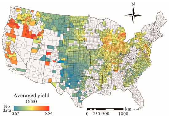
Figure 1.
The county-level average yield over years 2008–2018 of the winter wheat in the CONUS.
For most counties in the CONUS, winter wheat is generally planted in the fall [38] and it becomes established in the period of late autumn and winter. It then goes into dormancy and requires a process of vernalization until the following spring [39]. The plants recover in the spring and grow rapidly until the summer harvest. For modeling the winter wheat in the CONUS, a uniform growing season is needed and, therefore, we defined it as from the preceding October to the end of July of the current year. We used the previous two years’ yields as one type of the model inputs since the historical yields were found to be useful for crop yield prediction [20].
2.1.2. VI Data
Since the effectiveness of VIs had been previously validated for yield prediction [40,41,42], they were also considered in this study and derived from MODIS data. Specifically, the cloud free 16-day averaged daily MODIS MCD43A3 product, which provides a wealth of band information with 500-m spatial resolution, including the visible, near-infrared (NIR), and shortwave, was used for the VI extraction [43]. Four VIs that have been complementary and extensively used in crop yield analysis were calculated, including the NDVI, NDWI, EVI, and Green Chlorophyll Index (GCI). In particular, NDVI is widely used to assess vegetation vigor. NDWI is capable of extracting the moisture content of vegetation canopy. EVI is an optimized NDVI designed to improve the sensitivity of vegetation signals in areas with high biomass. GCI can indicate the canopy chlorophyll content and light use efficiency related to crop growth [44,45]. The four VIs were calculated while using Equations (1)–(4).
where NIR, Red, Green, and Blue represent the reflectance of the near-infrared, red, green, and blue bands, respectively; L is the canopy background adjustment; C1, C2 are the coefficients of the aerosol resistance term; and, G is the gain factor. The coefficients of EVI in Equation (3) were chosen according to the MODIS EVI algorithm, with L = 1, C1 = 6, C2 = 7.5, and G = 2.5 [46].
2.1.3. Climate Data
In addition to the widely adopted VIs, we also extracted the climate variables within the growing season from two gridded data sources, including the Parameter-elevation Regressions on Independent Slopes Model (PRISM) dataset [47] and MODIS Land Surface Temperature (LST) MOD11A2 product [48]. The primary meteorological variables were derived based on the PRISM dataset with 4 km spatial resolution. These variables include daily total precipitation (PPT), daily minimum and maximum vapor pressure deficit (VPDmn, VPDmx), daily minimum, maximum, and mean temperature (Tmn, Tmx, Tmean), and daily mean dew point temperature (TDmean). Two additional variables, including daytime and nighttime land surface temperature (LST_D, LST_N), were extracted from the MOD11A2 product, which is an eight-day composite data product with a 1 km spatial resolution. In sum, the extracted factors can be divided into two categories: (1) water-related factors including PPT, VPDmn, and VPDmx, (2) temperature-related factors, including Tmean, Tmn, Tmx, TDmean, LST_D, and LST_N.
2.1.4. Soil Data
Soil properties, such as soil moisture and nutrient, also significantly influence plant growth. In this study, six types of soil properties, including organic carbon content (SOC), total nitrogen (TN), bulk density (BD), pH, sand content (SC), and clay content (CC), were derived from the US_SoilGrids100m soil maps [49]. The maps were generated to provide an estimation of soil properties for the CONUS at seven different depths (0, 5, 15, 30, 60, 100, and 200 cm) that are spatially continuous and internally consistent at a 100-m spatial resolution. Each map describes one soil property at a certain depth. All of the maps are available and can be obtained from the Penn State University repository at https://scholarsphere.psu.edu [49]. We considered the six soil properties at all the seven depths since the winter wheat roots have shown to reach 200 cm depth [50].
2.1.5. Data Preprocessing
All of the extracted yield affecting factors, including the VIs, climate variables, and soil properties, were spatially aggregated to the county level, and the Cropland Data Layer (CDL) at 30-m resolution provided by NASS [51,52] was used to identify the wheat area and extract wheat fields. The daily sequential variables, including the climate data and VIs, were collected and aggregated to a 16-day interval during the growing season, resulting in a total of twenty temporal data records. The Google Earth Engine (GEE) platform [53] was used for these preprocessing steps. A total of 304 input variables were obtained for model development, including 260 for the sequential features (four VIs and nine climate variables with twenty temporal records for each), 42 for the six soil properties from seven depths, and two years of historical yields. We also showed the sample size for each year in Appendix A Figure A1, and “processed” samples in Figure A1 were used for the model development. The size difference among years is mainly due to two reasons. One is the long-term downward trend in winter wheat planting (Figure A1 “raw” samples), which is likely due to the growing foreign competition in international wheat markets [6]. Additionally, in each year, the samples with missing values in their features were removed from the model development.
2.2. Model Development and Performance Evaluation
The extracted variables were firstly explored, with the significant ones then applied for the model development, to build accurate and timely yield prediction models. Different machine learning models were then compared and evaluated. Next, the best model was selected for analyzing the multi-source data contribution and the near real-time prediction performance within the growing season. Specifically, the entire workflow consists of the following five main steps: (1) select the most informative input variables using correlation analysis; (2) construct prediction models using two linear regression (OLS and LASSO) and four machine learning methods (SVM, RF, AdaBoost, and DNN); (3) compare different models in terms of the prediction accuracy and the spatial adaptability; (4) investigate the contribution of multiple data sources; and, (5) evaluate the forecasting performance against timelines.
2.2.1. Strategy for Input Variable Selection
We first applied the Pearson correlation coefficient (PCC) to select the variables that mostly affect the yield to reduce the input data dimensionality. The PCC is a common method to measure the correlation degree between two variables, and an absolute value greater than 0.5 indicates good correlation [54].
Specifically, the PCCs were calculated between (1) each input variable and the yield and (2) any two variables within each data source. For the sequential VIs and climate data, the mean value of each time series variable was used for the calculation. Subsequently, two variables were selected from each data source based on the following criteria: (1) the variable that had the maximum absolute correlation with the yield was selected; and, (2) among the remaining factors, the one had a correlation with the previously selected variable below a threshold (0.5 in this study), while most correlated with the yield was also included. This strategy can ensure selecting the informative and diverse factors, in order to improve the efficiency while reducing the redundancy in modeling.
2.2.2. Machine Learning Algorithms for Yield Prediction
We explored two linear regression methods and four machine learning methods in this work. The dependent variable was the county-level winter wheat yield for the current year. The independent variables were the selected variables and they were normalized before the model development. The models were trained on the data from 2008 to 2016 and then the trained models were evaluated in 2017 and 2018. The scikit-learn library implemented six mainstream machine learning algorithms in Python, and a five-fold cross-validated grid search optimized their hyper-parameters using the “GridSearchCV” module in the library [55]. A brief description of each algorithm is presented below.
OLS is a commonly used linear algorithm that aims to minimize the sum of the square errors between the ground truth and the predicted value. However, OLS lacks penalties for the regression coefficients and, thus, might cause overfitting when there is a large number of input variables. LASSO, which was proposed by Tibshirani [56], is a shrinkage and selection algorithm for linear regression to reduce overfitting. It assumes that some independent variables are more important than the others. Based on the OLS, a L1 norm regularization was added to its loss function, which can not only reduce overfitting, but also removes redundant information in the inputs. The main hyper-parameter of the LASSO is the weighting parameter of the regularization term, and it was set to 0.2 in this study.
SVM is a class of algorithm characterized by the usage of kernels and proposed by Gunn [57]. There are two main steps in an SVM regression model. First, the variables are mapped from the original space to a high-dimensional feature space by a kernel function. The kernel function can be either linear or non-linear, and it is determined by the relationship between the independent and dependent variables. Second, a linear model is constructed in the derived feature space to minimize the errors [58]. The main hyper-parameters include kernel function, kernel coefficient, and regularizer weighting parameter, and they were assigned to “radial basis function (RBF)”, “0.1”, and “2”, respectively, in this work.
RF is an ensemble learning method that has been widely used in different applications [59,60,61]. It is constructed by a large set of decision trees, with each tree being built using a random set of features and samples. RF is a bagging algorithm in which the decision trees are learned in parallel and independent of each other, with the final prediction combining the results from each individual tree. Two critical hyper-parameters include the total number of trees and the maximum depth of each tree, which were set to 400 and 8, respectively.
AdaBoost is another ensemble learning method that was proposed by Freund and Schapire [62]. When compared to RF, it is a boosting algorithm in which the base learners are generated in a sequential way, and the final prediction is achieved by taking a weighted average of base learners. In each iteration, the training samples are assigned different weighting factors with more weight on misclassified instances, which allows for the AdaBoost to control the bias and variance. In this work, the decision tree was used as the base learner. The parameters include the maximum number of estimators, learning rate, and loss function were set to 400, 1, and “linear”, respectively.
Deep learning is a breakthrough technology in machine learning and data mining, which has a structure that provides sufficient ability to learn feature representations from the data [63]. There are different types of architectures, and our study applied the fully-connected DNN [64], which increases the depth of the conventional ANNs [65]. DNN contains one input layer, several hidden layers, and one output layer. Each layer has a collection of conceptualized neurons, which can move between layers through weighted connections and activation functions. In this study, we designed a seven-layered network, in which the number of neurons was set to 256, 128, 128, 64, and 24, respectively, in the five hidden layers. We used the “Relu” as the activation function and applied the “Dropout” strategy to improve the model generalization ability. Finally, we configured the model with the “adam” optimizer, the “mean_absolute_error” loss function, and set the learning rate as 0.001.
2.2.3. Metrics for Model Evaluation
We used the root mean squared error (RMSE), coefficient of determination (R2), and mean absolute error (MAE) to quantify the model prediction performance. Additionally, the spatial autocorrelation of prediction errors, which can be measured by the Global Moran’s I metric, reflects the model generalizability over the spatial domain, as demonstrated by previous studies [66,67,68,69]. The value of Global Moran’s I ranges from -1 to 1 [70], where positive values indicate a trend of aggregation and negative values indicate a trend of dispersion. Values that are near zero indicate spatial randomness patterns, with higher randomness indicating a better model [71]. In this study, we used ArcGIS 10.6 to calculate the Global Moran’s I.
3. Results
3.1. Important Factor Selection.
The PCC was calculated within each data source, except for the historical yields as only two previous years’ yields were considered in this study, as demonstrated by previous studies. Additionally, it worth noting that the climate variables were divided into two categories, with the water- and temperature-related variables in each. The correlation coefficients for each group are shown in Figure 2, and the corresponding p-values are shown in Appendix A Figure A2.
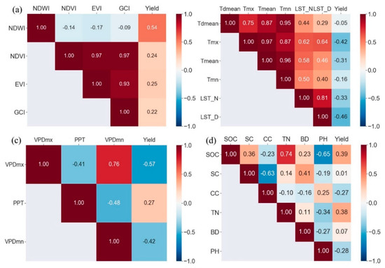
Figure 2.
Correlation matrices for different data sources: (a) VIs; (b) Temperature-related factors; (c) Water-related factors; and, (d) Soil properties.
Generally, the VIs all demonstrated positive correlations with the yield, while the temperature-related factors were negatively correlated with the yield. For the other two groups, both positive and negative correlations were observed. The method described in Section 2.2.1 was used to select important factors from each source. For example, within the VI group, NDWI and EVI were selected, because NDWI showed the strongest correlation with the yield; and, EVI had a correlation less than 0.5 with the selected NDWI while showing the highest correlation with the yield among the remaining three factors. Similarly, we selected LST_D and Tmean among the Temperature-related factors; VPDmx and PPT from the Water-related factors; and, SOC and CC within the soil properties.
3.2. Model Comparison
We trained the six models described in Section 2.2.2 using both the full and selected factors separately to compare the performances of different models and evaluate the effectiveness of the factor selection, and the accuracies on the testing data are reported in Table 2. First, the results showed that an RMSE of less than 0.7 t/ha, a MAE of less than 0.6 t/ha, and an R2 of more than 0.75 were found for all of the approaches, demonstrating the efficacy of using multi-source data for yield prediction. Subsequently, when comparing the different methods, we found that the non-linear machine learning approaches, in general, performed better than the two linear approaches, and the AdaBoost model outperformed all other approaches, achieving an R2 of 0.85 while using the full factors, and an R2 of 0.86 with the reduced factors. Regarding the factor selection, improvements were observed in most cases, and the R2 was significantly increased for the DNN model when the reduced factors were considered. This was primarily because reducing the input factors could significantly reduce the number of weights that need to be estimated in the neural network and, thus, helped to prevent overfitting and enhanced the model generalization ability.
Table 2.
The predictive performance of the six models using both full and selected factors (the highest accuracy was highlighted in bold).
In addition, Figure 3 further showed the agreement between the prediction and the reported yield of different models that were developed by the selected factors. The results were presented for both the training (red) and testing datasets (black). Again, among the six statistical models, the best agreement was found in the AdaBoost (Figure 3e), and the two linear methods showed less agreement than the other approaches (Figure 3 a,b). Besides, we also noticed that the yields were underestimated in some high-yield counties (green ellipses), notably in the OLS, LASSO, and SVM models. This is mainly because the quantity of high-yield samples was relatively small, which results in difficulty for modeling the yield variation. For the following analysis, we excluded the OLS model, as it consistently showed the worst performance among all of the approaches.
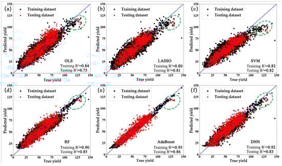
Figure 3.
The scatter plots of the six models using the selected factors (the green ellipses represent the underestimated regions): (a) OLS; (b) LASSO; (c): SVM; (d): RF; (e): AdaBoost; (f): DNN.
3.3. The Spatial Patterns of Predicted Yield
We further reported the predicted yields on the two testing years (2017 and 2018) in Figure 4, and the predictions were obtained by the five different models that were trained with the selected factors. In general, the spatial patterns of the predicted yield were consistent with the reality for all methods (Figure 4c–j), showing that high-yield counties were distributed in the west and east, while the yield in the central region was relatively low. Subsequently, when comparing the different approaches, we noticed that yields in the northeast region in the year of 2018 were underestimated in most models (black ellipses in Figure 4d,h,j,l), which were in agreement with the results shown in Figure 3, which was likely due to the reason of the small sample size of the high-yield counties. Additionally, it was seen that the predicted yield generated by the AdaBoost model (Figure 4e,f) had the most similar spatial patterns with the ground truth, while the linear LASSO model showed the worst, presenting both the underestimation in the northeast in 2018 (black ellipse in Figure 4l) and the significant overestimation in 2017 (red ellipse in Figure 4k).
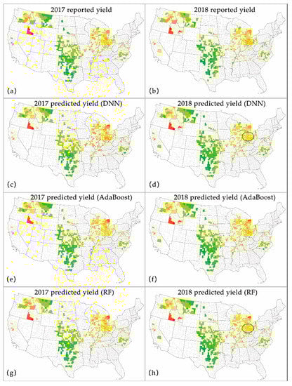
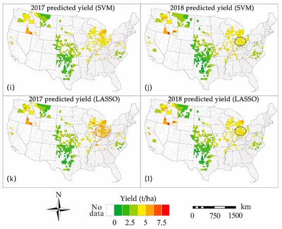
Figure 4.
The spatial patterns of the prediction (the black ellipses represent the underestimated regions. The red ellipse represents the overestimated region).
We also calculated the relative prediction error of each model to evaluate the adaptability of the models over the spatial domain, and the error maps are shown in Figure 5. For all of the approaches, the spatial clustering of overestimation (red ellipse) was observed in the central region in 2017, and the clustering of underestimation (black ellipse) was shown in west in 2018. The DNN, SVM, and LASSO had additional aggregation of underestimation in the east region in 2018, and the LASSO model showed a clustering of overestimation in the east in 2017 and in the central in 2018. We calculated the Moran’s I for the prediction errors of the five models to further quantify the error patterns (Table 3). The Moran’s I values of the models were all positive and the P-values were all less than 0.01, which indicated the spatial dependent and clustering distribution of the prediction errors. Among all of the approaches, the AdaBoost model showed the weakest clustering with the lowest Moran’s I value in 2017 (Moran’s I = 0.36, P < 0.01) and 2018 (Moran’s I = 0.32, P < 0.01), demonstrating its stronger spatial adaptability in comparison with other approaches.
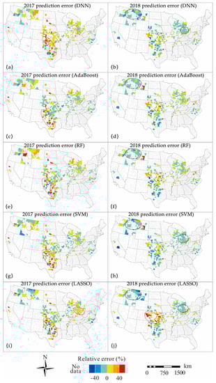
Figure 5.
The spatial patterns of the relative error (the black ellipses represent the spatial aggregation of underestimation. The red ellipses represent the spatial aggregation of overestimation).
Table 3.
Moran’s I of the prediction errors from different models (MI: Moran’s I; P: P-value).
3.4. Multi-Source Data Contribution
We further compared the developed multi-source based full model with several other reduced models that were built by using fewer data sources to demonstrate the effectiveness of using the multi-source data. In this analysis, the AdaBoost algorithm was considered due to its superior performance and only the selected factors from each data source were used for building the models. The prediction accuracies on the testing dataset, with different data source combinations, are shown in Figure 6. From the results, it was evident that the best performance was obtained when all of the data sources were combined, with an R2 of 0.86. Subsequently, within the single data source group, the best performance was achieved by using the soil data (R2 = 0.77), and the historical yields and sequential VIs showed slightly better performance than the climate. This was probably because the soil data had the finest spatial resolution, providing precise input for modeling, while the others are associated with more coarse resolutions, with 4 km for several climate variables (Tmean, PPT, VPDmx). In addition to the single source scenario, we also constructed two other reduced models while using the combination of sequential (VI and Climate) and non-sequential (soil and historical yields) factors. In both cases, the results outperformed the predictions that were obtained from the corresponding single data source, and an R2 of 0.8 was achieved when the soil and historical yields were combined. However, the time series factors were not able to explain more yield variation than the other case, which might also be due to the coarse spatial resolution of these variables.
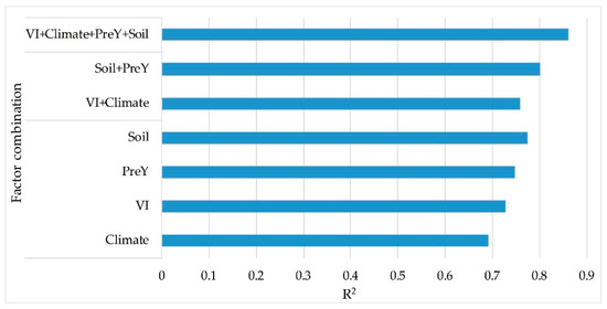
Figure 6.
The performance of the AdaBoost model using different combinations of the multi-source data.
3.5. Time-Series Prediction Performance
We then further investigate the model forecasting performance against timelines to achieve real-time yield prediction. Within the growing season, we compared the multi-source based full model with the reduced model only trained on the sequential data over time, and again, the AdaBoost algorithm was applied in all cases. The results were separately reported on the two testing years in Figure 7.
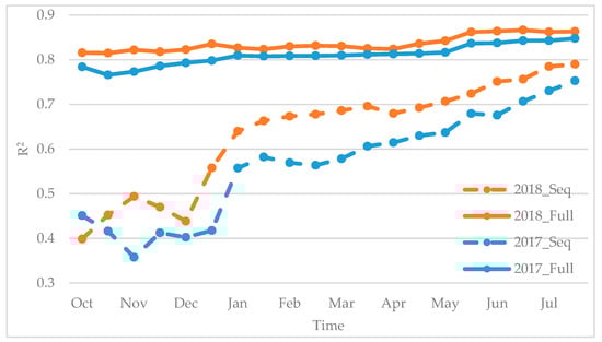
Figure 7.
The time-series performance of the AdaBoost model (Seq: using sequential data; Full: using all data).
When only considering the sequential data, the model accuracy significantly increased as time proceeds, and the best performance was achieved until harvest (July). Within the entire growing season, a noticeable accuracy improvement was observed between December and the following January, during which period the wheat starts the vernalization process, and then transits from vegetative growth to reproductive growth. During this period, the meterological conditions are essential for developing the wheat head size and, thus, play an important role in modeling the yield [72,73]. In addition, we also divided the entire growth period into three sub-seasons, including (1) Early season: from preceding October to December; (2) Middle season: from January to April; and, (3) Late season: from May to July, and the prediction results (Appendix A Table A1) also demonstrated that each phenological stage has a certain impact on the end-of-season yield and, thus, lacking the information from any stage would negatively affect the model performance.
In contrast, the full model showed different patterns. It outperformed the sequential model and showed robust performance within the entire growing season. This was largely because complementary information provided by the multi-source data can contribute to a more stable model. For example, the historical yields and soil properties, which were included in the full model, can provide prior knowledge for the yield potential, leading to a better performance in early-season prediction. In addition, although stable, noticeable improvements were still observed from mid-April to mid-May, during which the plants go through the heading, flowering, and early grain-filling stages. The model prediction capacity might be strengthened by the stronger correlation between the VIs with the yield during the flowering and grain-filling stages, as previously demonstrated [74,75]. Moreover, winter wheat is highly sensitive to the environmental stress during this stage [76,77], and climatic variables would significantly contribute to yield modeling within this period. These comparison results showed that the full model developed based on the multi-source data is more robust over time, and a high-performance prediction could be achieved in the middle of May, which is two and a half months before harvesting.
4. Discussion
4.1. Performance of Machine Learning Models
This study aimed to combine machine learning methods and multi-source data to predict the winter wheat yield in the CONUS. We used both the full and selected factors from the multi-source data to develop two linear and four machine learning models for yield prediction. The results indicated that factor selection played an important role in improving model performance, which was in agreement with previous studies [19,60]. We noticed that the OLS method had lower accuracy than all of the other methods and its performance cannot be improved through factor selection. This is because OLS is a basic linear method, and it is unable to process high dimensional data. Although LASSO is also a linear approach, it is constructed with a weight constraint process, thus resulting in a better performance when dealing with a large number of input variables.
The results also demonstrated that the machine learning methods were superior to the two linear methods, which was consistent with the previous studies demonstrating that machine learning methods are good at handling nonlinear and complex datasets [78,79]. Among the four machine learning models, the AdaBoost method achieved the highest accuracy in this study. DNN was inferior to the two ensemble learning methods (RF and AdaBoost) in this work, although it often outperforms traditional machine learning methods under a larger sample size [80,81]. This is mainly because the sample set, including the winter wheat growing-counties over 11 years (2008–2018) in the CONUS, was still relatively small for training the DNN model. RF outperformed the other models, except AdaBoost. This is probably because combining multiple base learners into one predictive model can help to decrease the variance [82]. In this study, the AdaBoost method performed better than RF, which was probably attributable to the boosting strategy, which pays more attention to the prediction error and generates a new tree to minimize that error.
4.2. Spatial Adaptability of Model Performance
The study found that, in some high-yield regions, the yields were underestimated in several models (Figure 3), which was in agreement with the previous studies [12,67,83]. This may be due to the small quantity of samples with high-yield or due to the fact that higher yield was typically associated with higher density, which might cause a saturation issue of optical remote sensing and thus affect the model performance. We also compared the spatial adaptability of different models using Global Morans’I, which showed that the prediction errors from all the models had some spatial aggregation, indicating that their performances vary over space. Our study predicted yield for the entire CONUS, and understandably such a large spatial scale typically introduces more complex environmental conditions and greater variability in planting conditions, which can also lead to unstable modeling performance in the spatial domain [84,85]. It is noteworthy that the spatial aggregation of the LASSO model was higher than the other machine learning methods, which indicated that this linear method was unable to model the complex spatial data [86,87]. Meanwhile, AdaBoost model exhibited the best performance in addressing the spatial variation with the lowest Moran’s I value, indicating that the boosting strategy not only improves overall accuracy, but also improves spatial adaptability.
4.3. Impact of Multi-Source Data on Yield Prediction
We first used the PCC method to analyze the correlation between the yield and the variables from multi-source data. The results showed that all of the VI factors were positively correlated with the yield, while the temperature-related factors showed negative correlations with the yield, which were consistent with the previous study [19]. This method allowed for us to find the important yield affecting factors, including the NDWI and EVI from the VIs; LSD_T, Tmean, VPDmx, and PPT from the climate variables; SOC and CC from the soil properties, and the previous two years of yields. With the selected factors from multi-source data, the AdaBoost model achieved the highest accuracy in this study.
We evaluated the contribution of different data sources in yield modeling. For the single data source, the soil factors could achieve a better performance than other data sources. Soil properties represent the fertility of soil, which directly affects the crop yield. Majchrzak et al. established a multiple regression to estimate the wheat yield while using 16 soil properties in Illinois, and the final model explained 78% variation in the wheat yield (R2 = 0.78) [88]. Our soil variables that were extracted at seven different depths provided more detailed information, leading to enhanced prediction performance. [89]. We also noticed that the combinations of multiple sources, in general, outperformed the single data source, with the full data sources achieving the best performance. However, when combining the VI and climate data, it underperformed the models using only the soil factors. One possible reason is that the resolutions of the VIs (500 m) and climate variables (4 km) were much lower than the soil maps (100 m), and such coarse resolution might fail to capture the variation within the target unit [19]. Finally, we found that multi-source data also played an important role in time-series prediction. As compared only using the sequential data (VIs and climate variables), the full model with multi-source data maintained stable accuracy over the growing season, but it also achieved good performance two and a half months before the harvest.
4.4. Uncertainties and Future Work
Like all models, there are some limitations to the current study and modeling methods. First, the spatial resolution of the remote sensing data used in this work was relatively coarse and may affect the accuracy of the yield prediction. For further studies, we would consider data with higher resolution, such as Landsat and Sentinel. Second, spatial autocorrelation was not considered in this modeling, and it was necessary to incorporate spatial analysis into the machine learning approaches in order to reduce the spatial clustering issue. Third, although this approach worked well in the CONUS, it would be necessary to test its adaptability for other crops and regions.
5. Conclusions
Because of the significant role of winter wheat in the U.S., it is essential to estimate its yield precisely and timely. For this purpose, we developed machine learning models to predict county-level winter wheat yield for the CONUS, by using multi-source data. The results indicated that machine learning methods outperformed statistical methods, and the AdaBoost method performed the best. In addition, we examined the spatial autocorrelation of prediction errors for different models and, again, the Adaboost model showed the least clustering pattern, indicating its stronger spatial adaptability in comparison with other approaches. Furthermore, we explored the contribution of different data sources, and demonstrated the efficacy of using the multi-source data. We also found that soil properties are more critical than other data sources. Finally, we evaluated the model performance in a simulated real-time manner, with the results indicating that a reliable prediction could be achieved two and a half months before harvest.
Author Contributions
Conceptualization, Y.W. and Z.Z.; Formal analysis, Y.W., Z.Z. and L.F.; Methodology, Y.W. and Z.Z.; Validation, Y.W.; Writing—original draft, Y.W. and Z.Z.; Writing—review & editing, Y.W., Z.Z., L.F., Q.D. and T.R. All authors have read and agreed to the published version of the manuscript.
Funding
Support for this research was provided by the USDA National Institute of Food and Agriculture, United States Department of Agriculture, Hatch project WIS03026; the University of Wisconsin–Madison, Office of the Vice Chancellor for Research and Graduate Education with funding from the Wisconsin Alumni Research Foundation; the China Scholarship Council (NO.201906270090); and the Wuhan University Graduates International Exchange Program (NO.201909).
Acknowledgments
The authors would like to thank the valuable comments and suggestions of the anonymous reviewers.
Conflicts of Interest
The authors declare no conflict of interest.
Appendix A

Figure A1.
The sample size of each year from 2008–2018 (“raw”: samples with yield records from USDA NASS; “processed”: samples with complete input variables).

Figure A2.
P-values for different data sources: (a) VIs; (b) Temperature-related factors; (c) Water-related factors; (d) Soil properties.
Table A1.
Model performance comparison using different sub-season combinations (“ES”: early season; “MS”: middle season; “LS”: late season).
Table A1.
Model performance comparison using different sub-season combinations (“ES”: early season; “MS”: middle season; “LS”: late season).
| ES | MS | ES + MS | LS | MS + LS | ES + MS + LS | |
|---|---|---|---|---|---|---|
| VI | 0.468 | 0.492 | 0.587 | 0.709 | 0.714 | 0.727 |
| Climate | 0.312 | 0.486 | 0.578 | 0.607 | 0.671 | 0.692 |
| VI + Climate | 0.496 | 0.644 | 0.678 | 0.742 | 0.756 | 0.760 |
References
- FAO. World Food and Agriculture Statistical Pocketbook; FAO: Rome, Italy, 2019. [Google Scholar]
- FAO. FAOSTAT. Available online: http://www.fao.org/faostat/zh/#data/QC (accessed on 2 December 2019).
- Lesk, C.; Rowhani, P.; Ramankutty, N. Influence of extreme weather disasters on global crop production. Nature 2016, 529, 84–87. [Google Scholar] [CrossRef] [PubMed]
- Franch, B.; Vermote, E.F.; Becker–Reshef, I.; Claverie, M.; Huang, J.; Zhang, J.; Justice, C.; Sobrino, J.A. Improving the timeliness of winter wheat production forecast in the United States of America, Ukraine and China using MODIS data and NCAR Growing Degree Day information. Remote Sens. Environ. 2015, 161, 131–148. [Google Scholar] [CrossRef]
- Statista. U.S. Imports and Exports of Wheat from 2000/01 to 2018/19 (in Million Metric Tons). Available online: https://www.statista.com/statistics/237902/us–wheat–imports–and–exports–since–2000/ (accessed on 2 December 2019).
- USDA. Wheat Sector at a Glance. Available online: https://www.ers.usda.gov/topics/crops/cotton-wool/cotton-sector-at-a-glance/ (accessed on 2 December 2019).
- Rembold, F.; Atzberger, C.; Savin, I.; Rojas, O. Using low resolution satellite imagery for yield prediction and yield anomaly detection. Remote Sens. 2013, 5, 1704–1733. [Google Scholar] [CrossRef]
- Sibley, A.M.; Grassini, P.; Thomas, N.E.; Cassman, K.G. Testing remote sensing approaches for assessing yield variability among maize fields. Agron. J. 2014, 106, 24–32. [Google Scholar] [CrossRef]
- Guan, K.Y.; Wu, J.; Kimball, J.S.; Anderson, M.C.; Frolking, S.; Li, B.; Hain, C.R.; Lobe, D.B. The shared and unique values of optical, fluorescence, thermal and microwave satellite data for estimating large–scale crop yields. Remote Sens. Environ. 2017, 199, 333–349. [Google Scholar] [CrossRef]
- Kayad, A.G.; Al-Gaadi, K.A.; Tola, E.; Madugundu, R.; Zeyada, A.M.; Kalaitzidis, C. Assessing the spatial variability of alfalfa yield using satellite imagery and ground–based data. PLoS ONE 2016, 11. [Google Scholar] [CrossRef]
- Ren, J.; Chen, Z.; Zhou, Q.; Tang, H. Regional yield estimation for winter wheat with MODIS–NDVI data in Shandong, China. Int. J. Appl. Earth Obs. Geoinf. 2008, 10, 403–413. [Google Scholar] [CrossRef]
- Becker–Reshef, I.; Vermote, E.; Lindeman, M.; Justice, C. A generalized regression–based model for forecasting winter wheat yields in Kansas and Ukraine using MODIS data. Remote Sens. Environ. 2010, 114, 1312–1323. [Google Scholar] [CrossRef]
- Kouadio, L.; Newlands, K.N.; Davidson, A.; Zhang, Y.; Chipanshi, A. Assessing the Performance of MODIS NDVI and EVI for Seasonal Crop Yield Forecasting at the Ecodistrict Scale. Remote Sens. 2014, 6, 10193–10214. [Google Scholar] [CrossRef]
- Holzman, M.E.; Rivas, R.; Piccolo, M.C. Estimating soil moisture and the relationship with crop yield using surface temperature and vegetation index. Int. J. Appl. Earth Obs. Geoinf. 2014, 28, 181–192. [Google Scholar] [CrossRef]
- Balaghi, R.; Tychon, B.; Eerens, H.; Jlibene, M. Empirical regression models using NDVI, rainfall and temperature data for the early prediction of wheat grain yields in Morocco. Int. J. Appl. Earth Obs. Geoinf. 2008, 10, 438–452. [Google Scholar] [CrossRef]
- Newlands, N.K.; Zamar, D.S.; Kouadio, L.A.; Zhang, Y.; Chipanshi, A.; Potgieter, A.; Toure, S.; Hill, H.S.J. An integrated, probabilistic model for improved seasonal forecasting of agricultural crop yield under environmental uncertainty. Front. Environ. Sci. 2014, 2, 17. [Google Scholar] [CrossRef]
- Ma, Y.; Kang, Y.; Ozdogan, M.; Zhang, Z. County–Level Corn Yield Prediction Using Deep Transfer Learning. In Proceedings of the AGU Fall Meeting 2019, San Francisco, CA, USA, 9–13 December 2019. [Google Scholar]
- Saeed, U.; Dempewolf, J.; Becker–Reshef, I.; Khan, A.; Ahmad, A.; Wajid, S.A. Forecasting wheat yield from weather data and MODIS NDVI using Random Forests for Punjab province, Pakistan. Int. J. Remote Sens. 2017, 38, 4831–4854. [Google Scholar] [CrossRef]
- Cai, Y.; Guan, K.; Lobell, D.; Potgieter, A.B.; Wang, S.; Peng, J.; Xu, T.; Asseng, S.; Zhang, Y.; You, L.; et al. Integrating satellite and climate data to predict wheat yield in Australia using machine learning approaches. Agric. For. Meteorol. 2019, 274, 144–159. [Google Scholar] [CrossRef]
- Zhang, Z.; Jin, Y.; Chen, B.; Brown, P. California Almond Yield Prediction at the Orchard Level With a Machine Learning Approach. Front. Plant Sci. 2019, 10, 809. [Google Scholar] [CrossRef] [PubMed]
- Ritchie, J.T.O. Description and performance of CERES wheat: A user—Oriented wheat yield model. ARS Wheat Yield Proj. 1985, 159–175. [Google Scholar]
- Jamieson, P.D.; Porter, J.R.; Wilson, D.R. A test of the computer simulation model ARCWHEAT1 on wheat crops grown in New Zealand. Field Crop. Res. 1991, 27, 337–350. [Google Scholar] [CrossRef]
- Hansen, S.; Jensen, H.E.; Nielsen, N.E.; Svendsen, H. Simulation of nitrogen dynamics and biomass production in winter wheat using the Danish simulation model DAISY. Fertil. Res. 1991, 27, 245–259. [Google Scholar] [CrossRef]
- Jamieson, P.D.; Semenov, M.A.; Brooking, I.R.; Francis, G.S. Sirius: A mechanistic model of wheat response to environmental variation. Eur. J. Agron. 1998, 8, 161–179. [Google Scholar] [CrossRef]
- Porter, J.R. AFRCWHEAT2: A model of the growth and development of wheat incorporating responses to water and nitrogen. Eur. J. Agron. 1993, 2, 69–82. [Google Scholar] [CrossRef]
- Moriondo, M.; Maselli, F.; Bindi, M. A simple model of regional wheat yield based on NDVI data. Eur. J. Agron. 2007, 26, 266–274. [Google Scholar] [CrossRef]
- Lobell, D.B.; Burke, M.B. On the use of statistical models to predict crop yield responses to climate change. Agric. For. Meteorol. 2010, 150, 1443–1452. [Google Scholar] [CrossRef]
- Wall, L.; Larocque, D.; Léger, P.M. The early explanatory power of NDVI in crop yield modelling. Int. J. Remote Sens. 2008, 29, 2211–2225. [Google Scholar] [CrossRef]
- Dubey, R.P.; Ajwani, N.; Kalubarme, M.H.; Sridhar, V.N.; Navalgund, R.R.; Mahey, R.K.; Sidhu, S.S.; Jhorar, O.P.; Cheema, S.S.; Na Rang, R.S. Pre–harvest wheat yield and production estimation for the Punjab, India. Int. J. Remote Sens. 1994, 15, 2137–2144. [Google Scholar] [CrossRef]
- Sridhar, V.N.; Dadhwal, V.K.; Chaudhari, K.N.; Sharma, R.; Bairagi, G.D.; Sharma, A.K. Wheat production forecasting for a predominantly unirrigated region in Madhya Pradesh. Titleremote Sens. 1994, 15, 1307–1316. [Google Scholar] [CrossRef]
- Forecasting, Y. Analysis of GAC NDVI data for cropland identification and yield forecasting in Mediterranean African countries. Photogramm. Eng. Remote Sens. 2001, 67, 593–602. [Google Scholar]
- Doraiswamy, P.C.; Moulin, S.; Cook, P.W.; Stern, A. Crop yield assessment from remote sensing. Photogramm. Eng. Remote Sens. 2003, 69, 665–674. [Google Scholar] [CrossRef]
- Heremans, S.; Dong, Q.; Zhang, B.; Bydekerke, L.; Van Orshoven, J. Potential of ensemble tree methods for early–season prediction of winter wheat yield from short time series of remotely sensed normalized difference vegetation index and in situ meteorological data. J. Appl. Remote Sens. 2015, 9. [Google Scholar] [CrossRef]
- Zhang, Y.; Qin, Q.; Ren, H.; Sun, Y.; Li, M.; Zhang, T.; Ren, S. Optimal Hyperspectral Characteristics Determination for Winter Wheat Yield Prediction. Remote Sens. 2018, 10, 2015. [Google Scholar] [CrossRef]
- Safa, M.; Samarasinghe, S.; Nejat, M. Prediction of wheat production using artificial neural networks and investigating indirect factors affecting it: Case study in Canterbury province, New Zealand. J. Agric. Sci. Technol. 2015, 17, 791–803. [Google Scholar]
- Wang, L.A.; Zhou, X.; Zhu, X.; Dong, Z.; Guo, W. Estimation of biomass in wheat using random forest regression algorithm and remote sensing data. Crop J. 2016, 4, 212–219. [Google Scholar] [CrossRef]
- NASS. NASS Quick Stats. In USDA National Agricultural Statistics Service (NASS). Available online: http://quickstats.nass.usda.gov/ (accessed on 8 December 2019).
- USDA–NASS. Field Crops: Usual Planting and Harvesting Dates. In USDA National Agricultural Statistics Service, Agriculural Handbook; NASS: Burr Ridge, IL, USA, 2010. [Google Scholar]
- Miller, T.D. Growth Stages of Wheat: Identification and Understanding Improve Crop Management. Better Crops 1992, 76, 12–17. [Google Scholar]
- Son, N.T.; Chen, C.F.; Chen, C.R.; Minh, V.Q.; Trung, N.H. A comparative analysis of multitemporal MODIS EVI and NDVI data for large–scale rice yield estimation. Agric. For. Meteorol. 2014, 197, 52–64. [Google Scholar] [CrossRef]
- Bolton, D.K.; Friedl, M.A. Forecasting crop yield using remotely sensed vegetation indices and crop phenology metrics. Agric. For. Meteorol. 2013, 173, 74–84. [Google Scholar] [CrossRef]
- Peng, Y.; Gitelson, A.A. Application of chlorophyll–related vegetation indices for remote estimation of maize productivity. Agric. For. Meteorol. 2011, 151, 1267–1276. [Google Scholar] [CrossRef]
- Schaaf, C.; Wang, Z. MCD43A3 MODIS/Terra+ Aqua BRDF/Albedo Daily L3 Global—500 m V006; NASA: Washington, DC, USA, 2015.
- Gitelson, A.A.; Vina, A.; Ciganda, V.; Rundquist, D.C.; Arkebauer, T.J. Remote estimation of canopy chlorophyll content in crops. Geophys. Res. Lett. 2005, 32. [Google Scholar] [CrossRef]
- Wu, C.; Niu, Z.; Gao, S. The potential of the satellite derived green chlorophyll index for estimating midday light use efficiency in maize, coniferous forest and grassland. Ecol. Indic. 2012, 14, 66–73. [Google Scholar] [CrossRef]
- Jiang, Z.; Huete, A.; Didan, K.; Miura, T. Development of a two–band enhanced vegetation index without a blue band. Remote Sens. Environ. 2008, 112, 3833–3845. [Google Scholar] [CrossRef]
- PRISM. Climate Group; Oregon State University: Corvallis, OR, USA, 2019. [Google Scholar]
- Wan, Z.; Hook, S.; Hulley, G. MOD11A2 MODIS/Terra Land Surface Temperature/Emissivity 8–day L3 Global 1 km SIN Grid V006; LP DAAC: Sioux Falls, SD, USA, 2015.
- Ramcharan, A.; Hengl, T.; Nauman, T.; Brungard, C.; Waltman, S.; Wills, S.; Thompson, J. Soil Property and Class Maps of the Conterminous United States at 100–Meter Spatial Resolution. Soil Sci. Soc. Am. J. 2018, 82. [Google Scholar] [CrossRef]
- Thorup–Kristensen, K.; Salmerón Cortasa, M.; Loges, R. Winter wheat roots grow twice as deep as spring wheat roots, is this important for N uptake and N leaching losses? Plant Soil 2009, 322, 101–114. [Google Scholar] [CrossRef]
- USDA–NASS. USDA National Agricultural Statistics Service Cropland Data Layer. Available online: https://nassgeodata.gmu.edu/CropScape/ (accessed on 8 December 2019).
- Boryan, C.; Yang, Z.; Mueller, R.; Craig, M. Monitoring US agriculture: The US department of agriculture, national agricultural statistics service, cropland data layer program. Geocarto Int. 2011, 26, 341–358. [Google Scholar] [CrossRef]
- Gorelick, N.; Hancher, M.; Dixon, M.; Ilyushchenko, S.; Thau, D.; Moore, R. Google Earth Engine: Planetary–scale geospatial analysis for everyone. Remote Sens. Environ. 2017, 202, 18–27. [Google Scholar] [CrossRef]
- Evans, J.D. Straightforward Statistics for the Behavioral Sciences; Thomson Brooks/Cole Publishing Co: Three Lakes, WI, USA, 1996. [Google Scholar]
- Buitinck, L.; Louppe, G.; Blondel, M.; Pedregosa, F.; Mueller, A.; Grisel, O.; Niculae, V.; Prettenhofer, P.; Gramfort, A.; Grobler, J. API design for machine learning software: Experiences from the scikit–learn project. arXiv 2013, arXiv:1309.0238. [Google Scholar]
- Tibshirani, R. Regression shrinkage and selection via the lasso. J. R. Stat. Soc. Ser. B 1996, 58, 267–288. [Google Scholar] [CrossRef]
- Gunn, S.R. Support vector machines for classification and regression. ISIS Tech. Rep. 1998, 14, 5–16. [Google Scholar]
- Smola, A.J.; Schölkopf, B. A tutorial on support vector regression. Stat. Comput. 2004, 14, 199–222. [Google Scholar] [CrossRef]
- Breiman, L.J.M.l. Random forests. Mach. Learn. 2001, 45, 5–32. [Google Scholar] [CrossRef]
- Sinha, P.; Gaughan, A.E.; Stevens, F.R.; Nieves, J.J.; Sorichetta, A.; Tatem, A.J. Assessing the spatial sensitivity of a random forest model: Application in gridded population modeling. Comput. Environ. Urban Syst. 2019, 75, 132–145. [Google Scholar] [CrossRef]
- Wang, Y.; Wu, X.; Chen, Z.; Ren, F.; Feng, L.; Du, Q. Optimizing the Predictive Ability of Machine Learning Methods for Landslide Susceptibility Mapping Using SMOTE for Lishui City in Zhejiang Province, China. Int. J. Environ. Res. Public Health 2019, 16, 368. [Google Scholar] [CrossRef]
- Freund, Y.; Schapire, R.E. A decision–theoretic generalization of on–line learning and an application to boosting. J. Comput. Syst. Sci. 1997, 55, 119–139. [Google Scholar] [CrossRef]
- Zhong, L.; Hu, L.; Zhou, H. Deep learning based multi–temporal crop classification. Remote Sens. Environ. 2019, 221, 430–443. [Google Scholar] [CrossRef]
- Biganzoli, E.; Boracchi, P.; Mariani, L.; Marubini, E. Feed forward neural networks for the analysis of censored survival data: A partial logistic regression approach. Stat. Med. 1998, 17, 1169–1186. [Google Scholar] [CrossRef]
- Rojas, R. Neural Networks: A Systematic Introduction; Springer Science & Business Media: Berlin, Germany, 2013. [Google Scholar]
- Peralta, N.; Assefa, Y.; Du, J.; Barden, C.; Ciampitti, I. Mid–season high–resolution satellite imagery for forecasting site–specific corn yield. Remote Sens. 2016, 8, 848. [Google Scholar] [CrossRef]
- Maimaitijiang, M.; Sagan, V.; Sidike, P.; Hartling, S.; Esposito, F.; Fritschi, F.B. Soybean yield prediction from UAV using multimodal data fusion and deep learning. Remote Sens. Environ. 2020, 237. [Google Scholar] [CrossRef]
- Imran, M.; Stein, A.; Zurita–Milla, R. Using geographically weighted regression kriging for crop yield mapping in West Africa. Int. J. Geogr. Inf. Sci. 2015, 29, 234–257. [Google Scholar] [CrossRef]
- Cai, R.; Yu, D.; Oppenheimer, M. Estimating the Spatially Varying Responses of Corn Yields toWeather Variations using GeographicallyWeighted Panel Regression. J. Agric. Resour. Econ. 2014, 39, 230–252. [Google Scholar]
- Moran, P.A.P. Notes on continuous stochastic phenomena. Biometrika 1950, 37, 17–23. [Google Scholar] [CrossRef]
- Maimaitijiang, M.; Ghulam, A.; Sandoval, J.S.O.; Maimaitiyiming, M. Drivers of land cover and land use changes in St. Louis metropolitan area over the past 40 years characterized by remote sensing and census population data. Int. J. Appl. Earth Obs. Geoinf. 2015, 35, 161–174. [Google Scholar] [CrossRef]
- Herbek, J.; Lee, C. A Comprehensive Guide to Wheat Management in Kentucky; University of Kentucky: Lexington, KY, USA, 2009. [Google Scholar]
- Wu, X.; Liu, H.; Li, X.; Tian, Y.; Mahecha, M.D. Responses of Winter Wheat Yields to Warming–Mediated Vernalization Variations Across Temperate Europe. Front. Ecol. Evol. 2017, 5, 126. [Google Scholar] [CrossRef]
- Fontana, D.C.; Potgieter, A.B.; Apan, A. Assessing the relationship between shire winter crop yield and seasonal variability of the MODIS NDVI and EVI images. Appl. GIS 2007, 3, 1–16. [Google Scholar]
- Labus, M.P.; Nielsen, G.A.; Lawrence, R.L.; Engel, R.; Long, D.S. Wheat yield estimates using multi–temporal NDVI satellite imagery. Int. J. Remote Sens. 2002, 23, 4169–4180. [Google Scholar] [CrossRef]
- Slafer, G.A.; Savin, R. Developmental base temperature in different phenological phases of wheat (Triticum aestivum). J. Exp. Bot. 1991, 42, 1077–1082. [Google Scholar] [CrossRef]
- Garg, D.; Sareen, S.; Dalal, S.; Tiwari, R.; Singh, R. Grain filling duration and temperature pattern influence on the performance of wheat genotypes under late planting. Cereal Res. Commun. 2013, 41, 500–507. [Google Scholar] [CrossRef]
- Feng, L.; Li, Y.; Wang, Y.; Du, Q. Estimating hourly and continuous ground–level PM2. 5 concentrations using an ensemble learning algorithm: The ST–stacking model. Atmos. Environ. 2019, 223, 117242. [Google Scholar] [CrossRef]
- Chlingaryan, A.; Sukkarieh, S.; Whelan, B. Machine learning approaches for crop yield prediction and nitrogen status estimation in precision agriculture: A review. Comput. Electron. Agric. 2018, 151, 61–69. [Google Scholar] [CrossRef]
- Kang, H.-W.; Kang, H.-B. Prediction of crime occurrence from multi–modal data using deep learning. PLoS ONE 2017, 12, e0176244. [Google Scholar] [CrossRef]
- Zhang, N.; Rao, R.S.P.; Salvato, F.; Havelund, J.F.; Møller, I.M.; Thelen, J.J.; Xu, D. MU–LOC: A machine–learning method for predicting mitochondrially localized proteins in plants. Front. Plant Sci. 2018, 9, 634. [Google Scholar] [CrossRef]
- Borchani, H.; Varando, G.; Bielza, C.; Larrañaga, P. A survey on multi-output regression. Wiley Interdiscip. Rev. Data Min. Knowl. Discov. 2015, 5, 216–233. [Google Scholar] [CrossRef]
- Vergara–Díaz, O.; Zaman–Allah, M.A.; Masuka, B.; Hornero, A.; Zarco–Tejada, P.; Prasanna, B.M.; Cairns, J.E.; Araus, J.L. A novel remote sensing approach for prediction of maize yield under different conditions of nitrogen fertilization. Front. Plant Sci. 2016, 7, 666. [Google Scholar] [CrossRef]
- Tao, F.; Xiao, D.; Zhang, S.; Zhang, Z.; Rötter, R.P. Wheat yield benefited from increases in minimum temperature in the Huang–Huai–Hai Plain of China in the past three decades. Agric. For. Meteorol. 2017, 239, 1–14. [Google Scholar] [CrossRef]
- Zhao, Y.; Lobell, D.B. Assessing the heterogeneity and persistence of farmers’ maize yield performance across the North China Plain. Field Crop. Res. 2017, 205, 55–66. [Google Scholar] [CrossRef]
- Nawar, S.; Buddenbaum, H.; Hill, J.; Kozak, J. Modeling and mapping of soil salinity with reflectance spectroscopy and landsat data using two quantitative methods (PLSR and MARS). Remote Sens. 2014, 6, 10813–10834. [Google Scholar] [CrossRef]
- Wang, J.; Ding, J.; Abulimiti, A.; Cai, L. Quantitative estimation of soil salinity by means of different modeling methods and visible–near infrared (VIS–NIR) spectroscopy, Ebinur Lake Wetland, Northwest China. PeerJ 2018, 6, e4703. [Google Scholar] [CrossRef] [PubMed]
- Majchrzak, R.N.; Olson, K.R.; Bollero, G.; Nafziger, E.D. Using soil properties to predict wheat yields on Illinois soils. Soil Sci. 2001, 166, 267–280. [Google Scholar] [CrossRef]
- De La Rosa, D.; Cardona, F.; Almorza, J. Crop yield predictions based on properties of soils in Sevilla, Spain. Geoderma 1981, 25, 267–274. [Google Scholar] [CrossRef]
© 2020 by the authors. Licensee MDPI, Basel, Switzerland. This article is an open access article distributed under the terms and conditions of the Creative Commons Attribution (CC BY) license (http://creativecommons.org/licenses/by/4.0/).