Different Spectral Domain Transformation for Land Cover Classification Using Convolutional Neural Networks with Multi-Temporal Satellite Imagery

 , ,
, ,
Abstract

1. Introduction
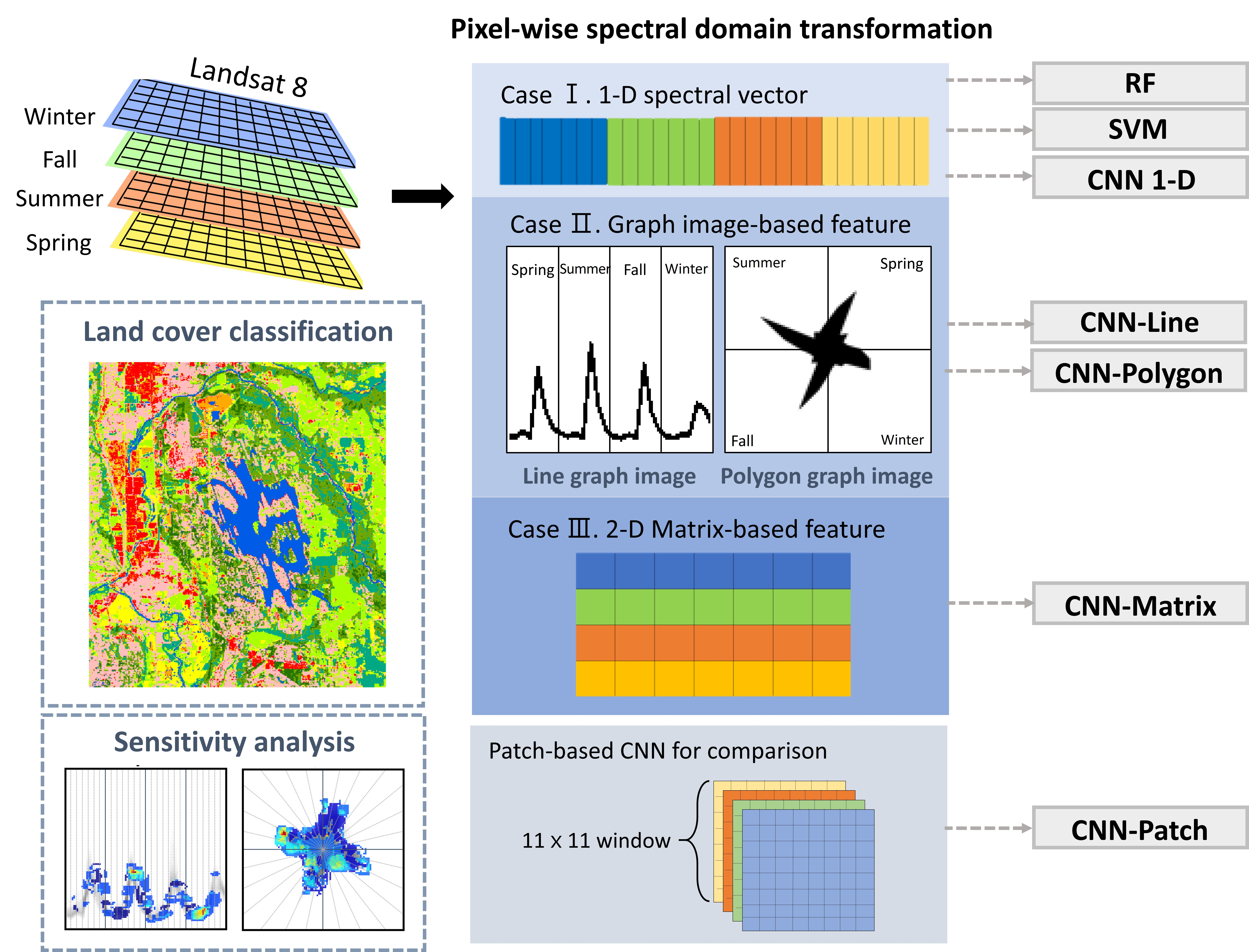
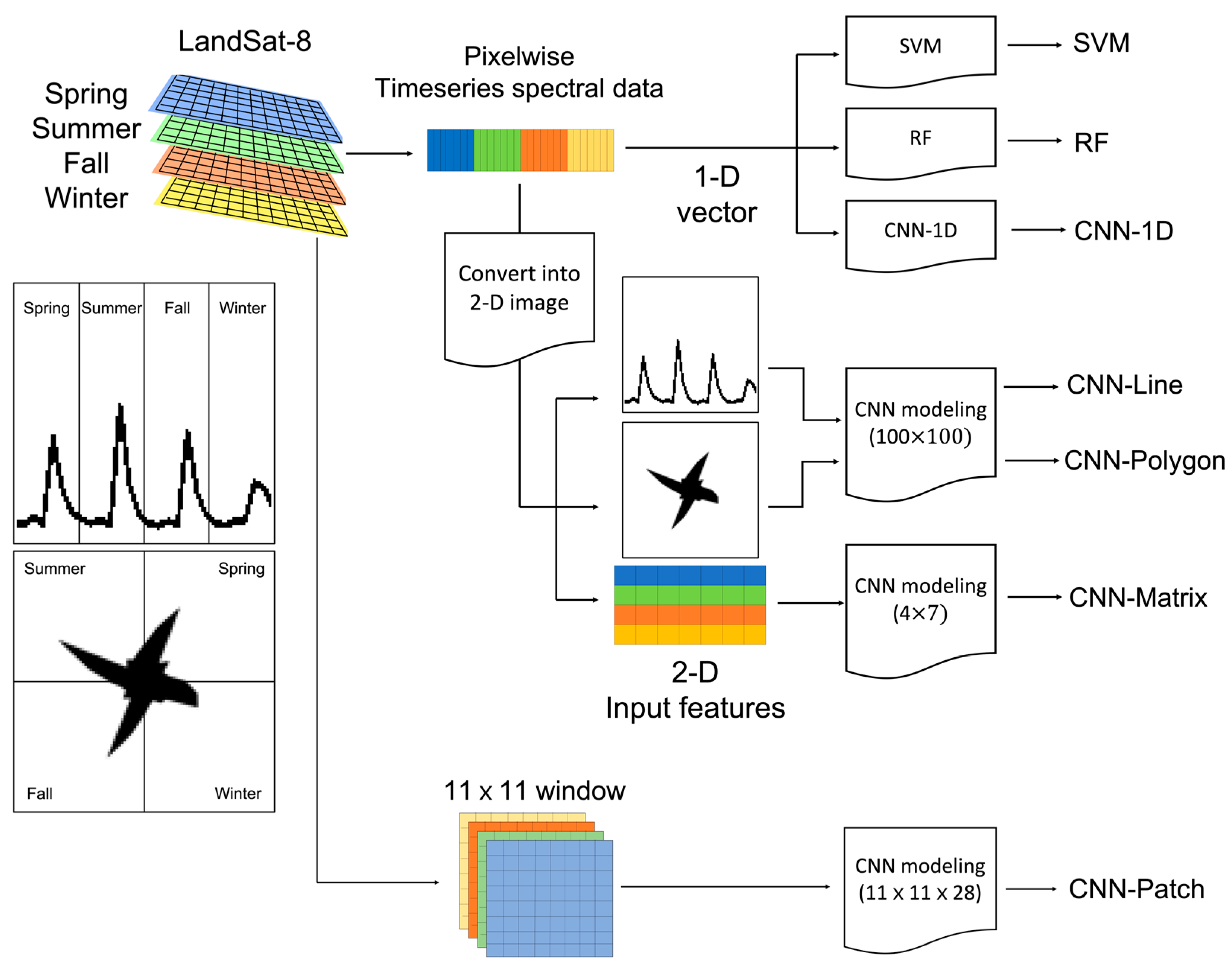
2. Proposed Methods
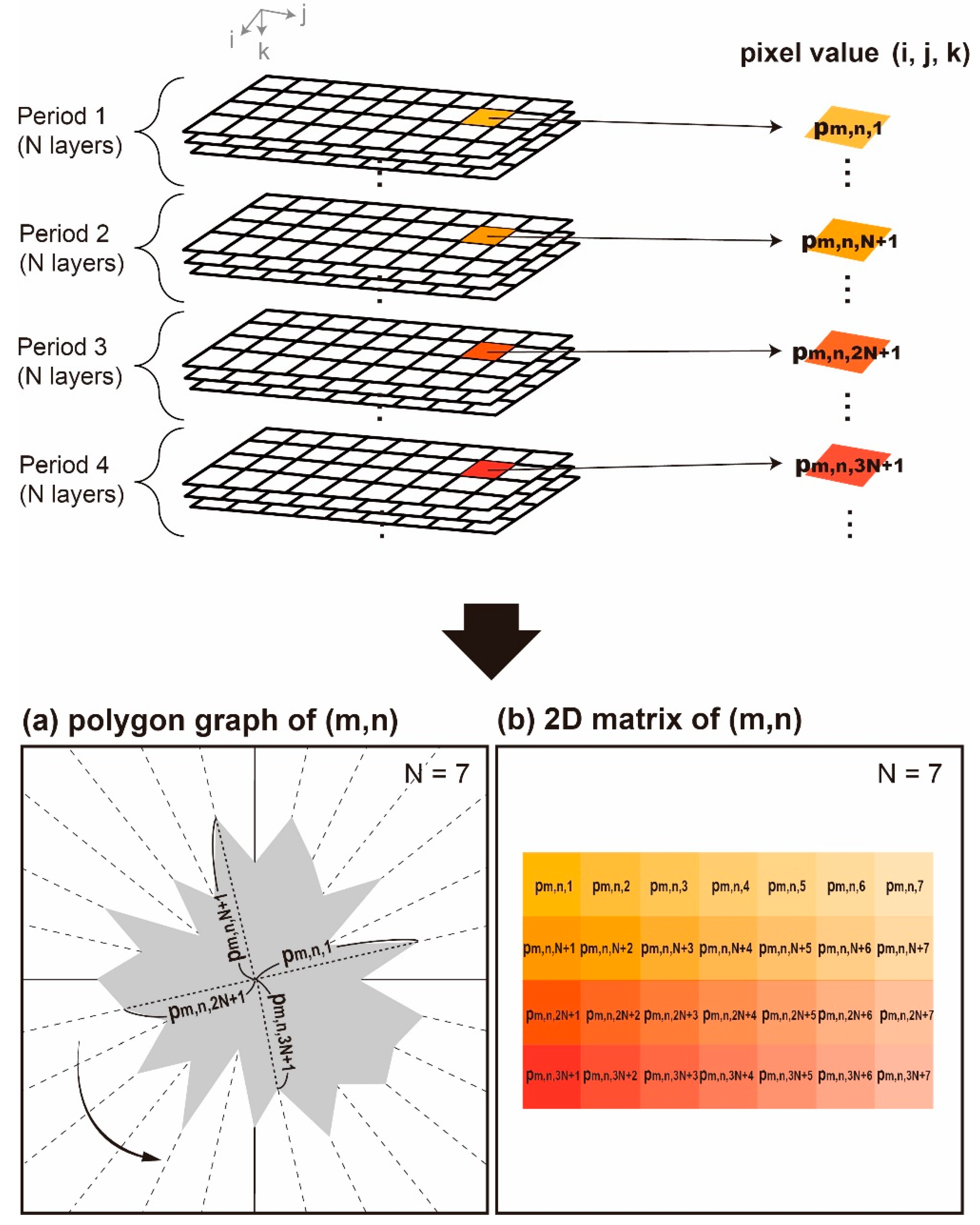
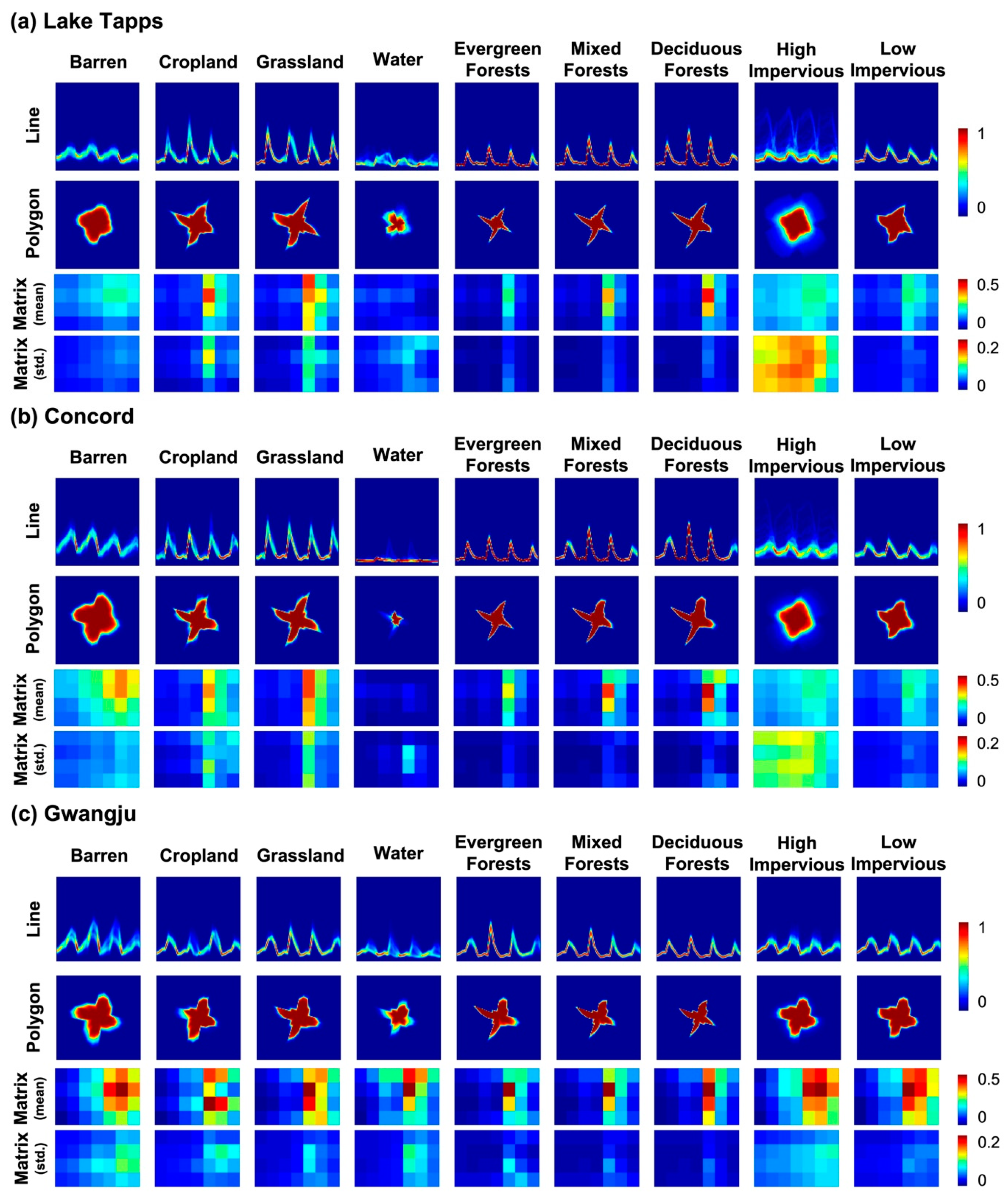
2.1. 2-D Feature Extraction
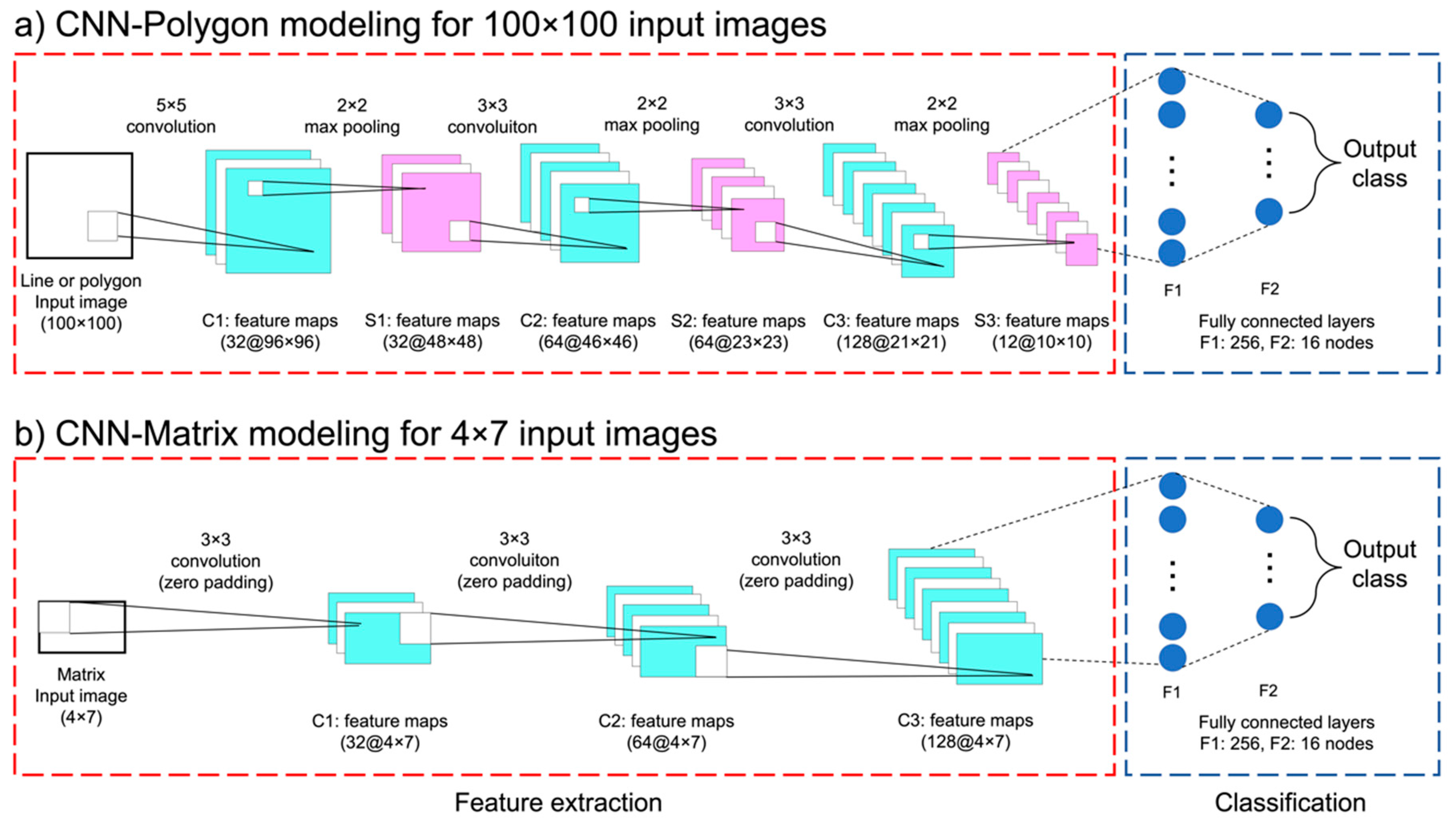
2.2. Convolutional Neural Networks
2.3. CNN Architecture
3. Study Areas and Data
3.1. Study Areas
3.2. Ground Reference Data
3.3. Landsat 8 Images
4. Experimental Design
5. Results
5.1. Model Performance
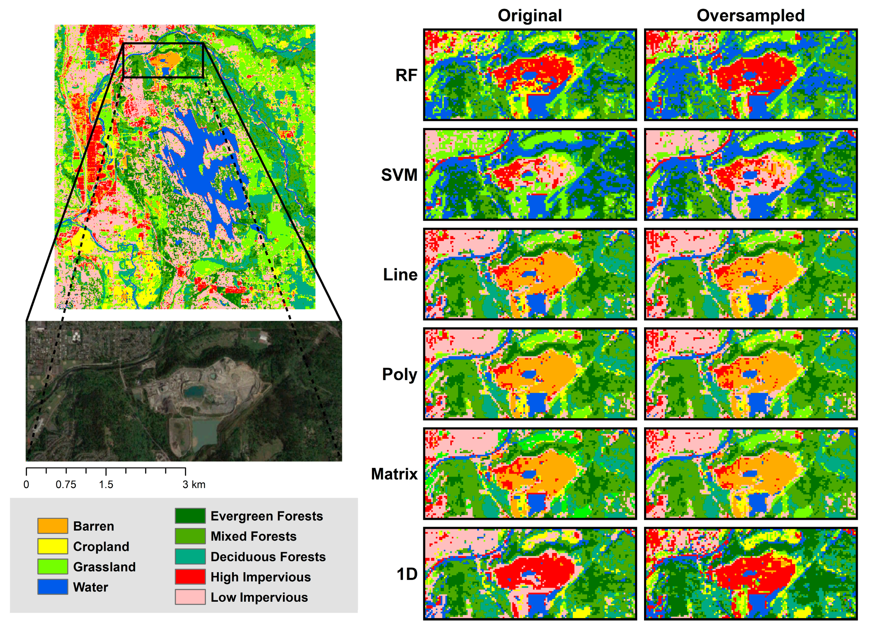
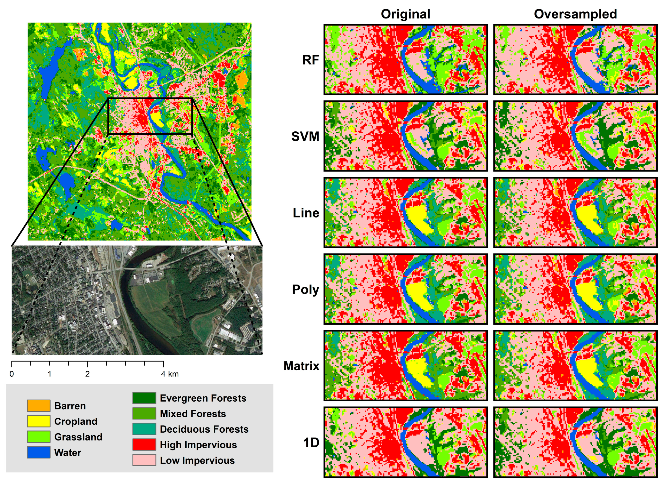
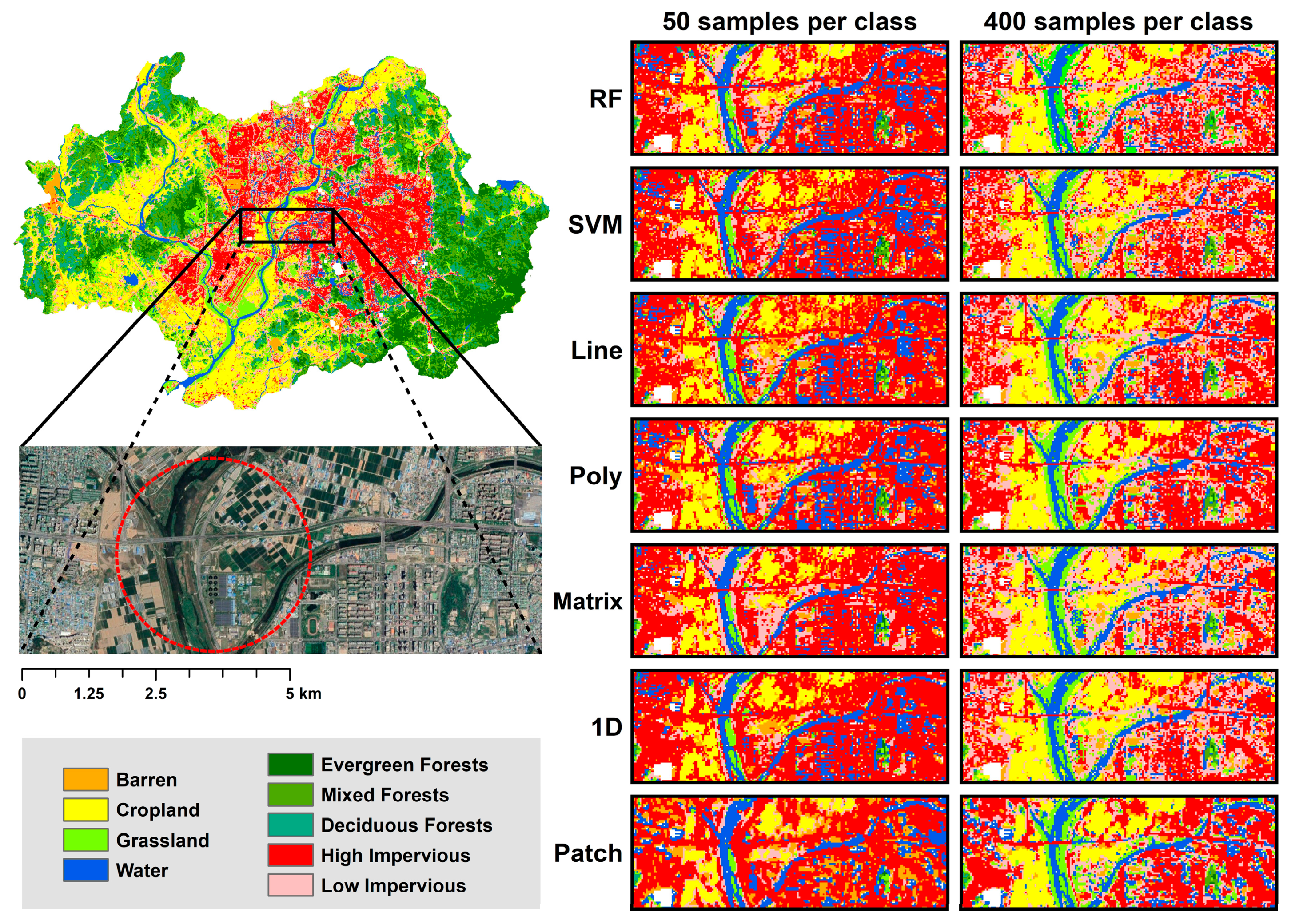
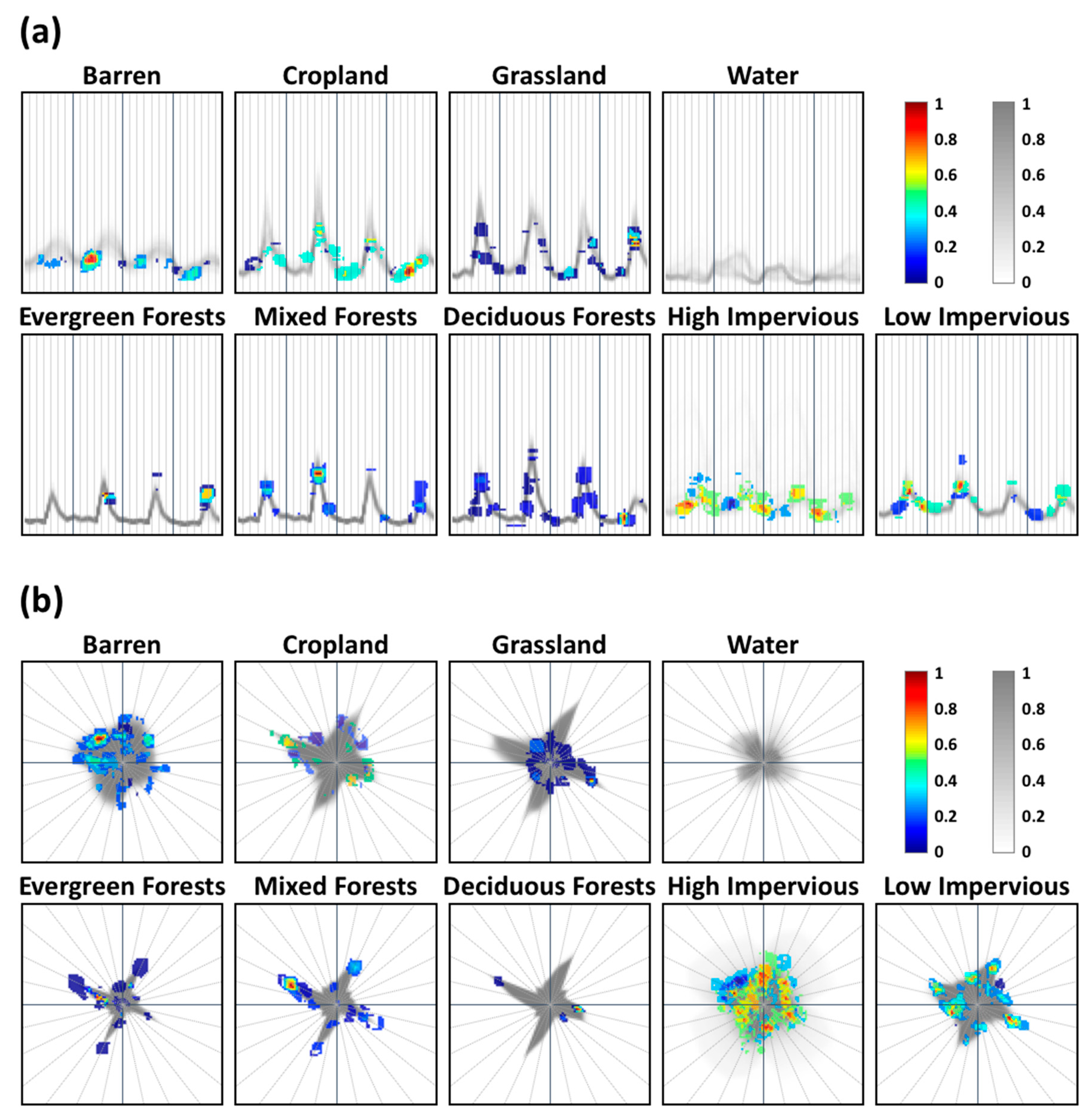
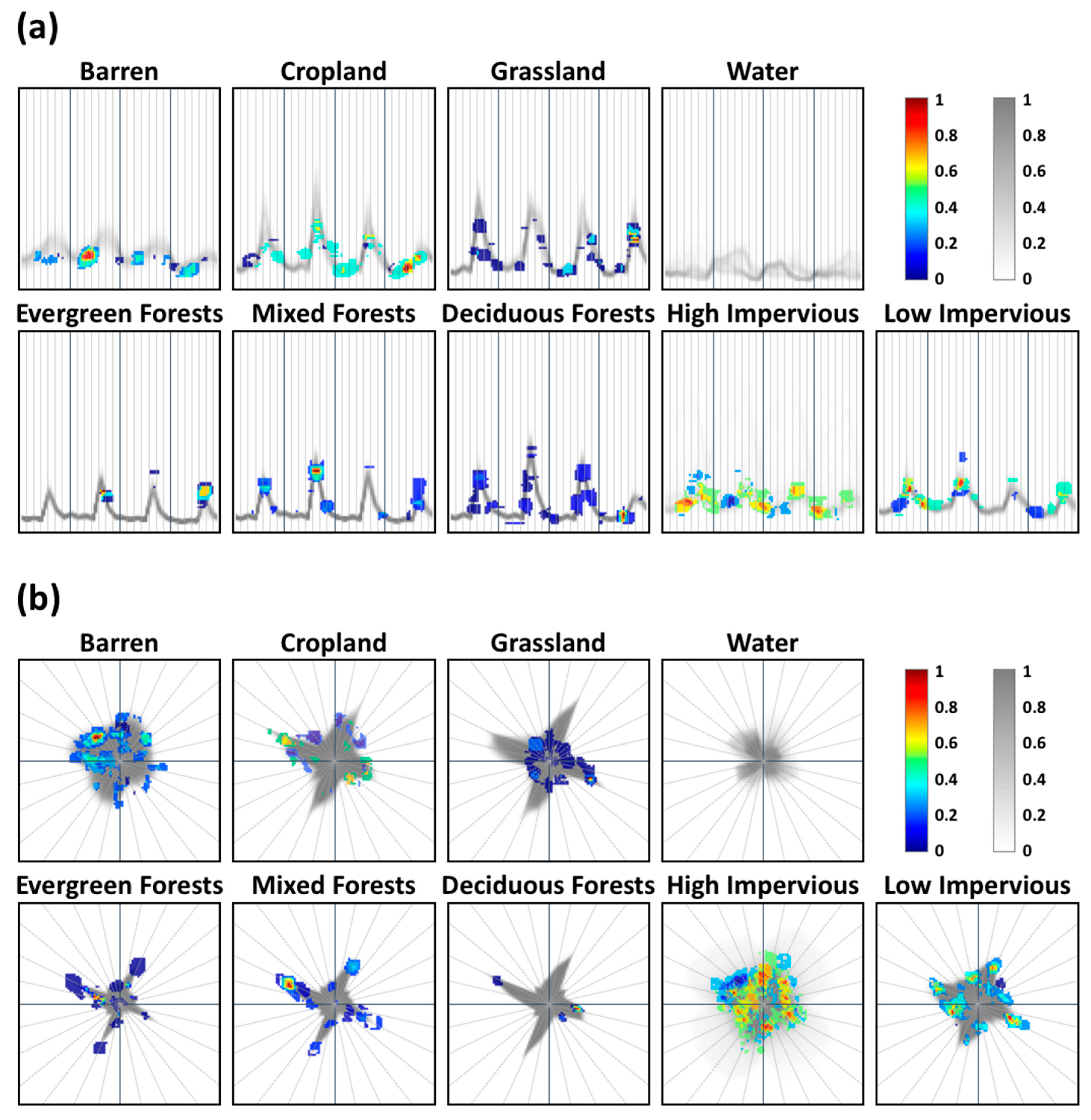
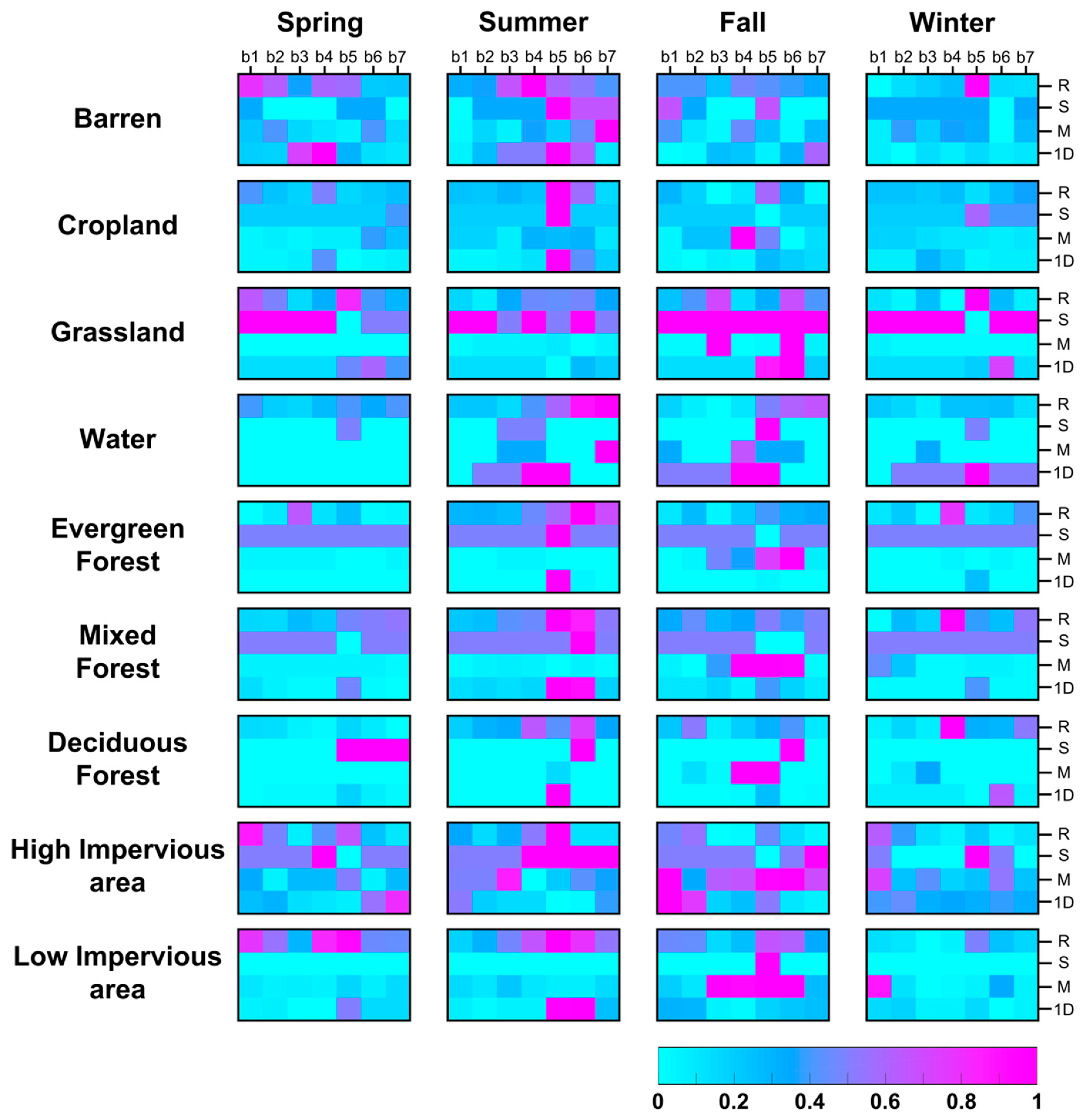
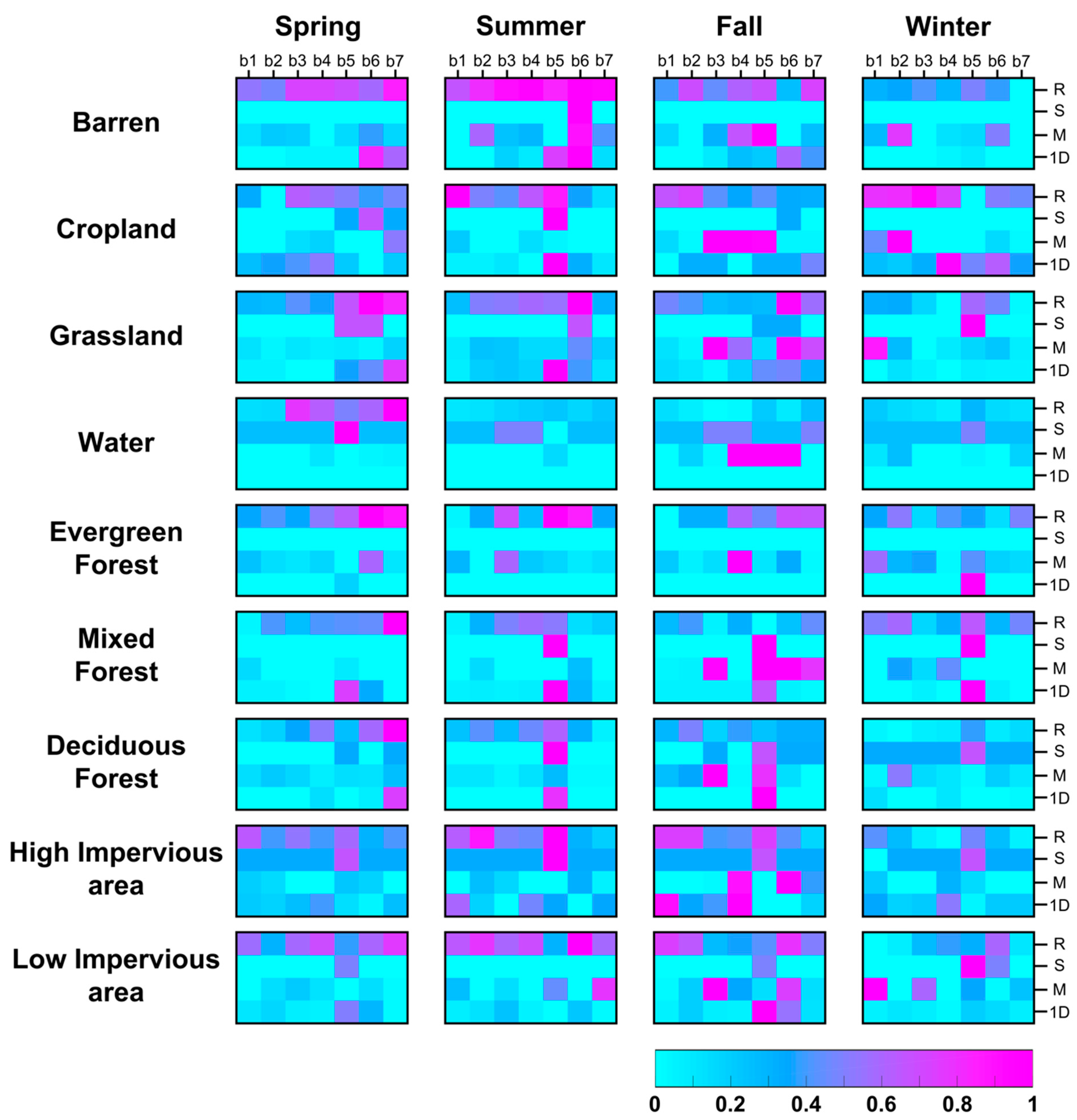
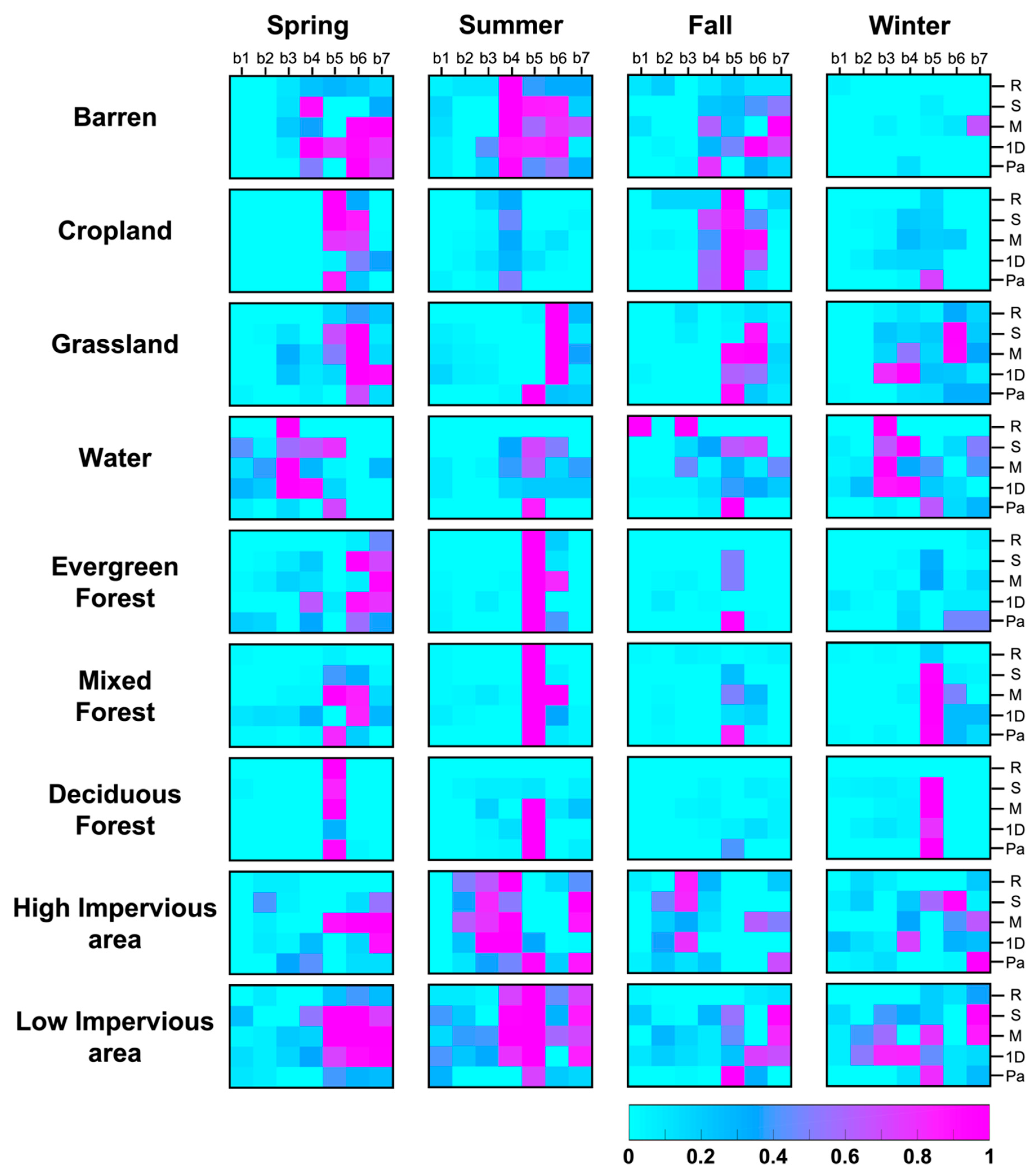
5.2. Sub-Class Analysis with Land Cover Classification Maps
6. Discussion
6.1. Model Type, Sample Size, and Performance
6.2. Sensitivity Analysis
6.3. Novelty and Limitations
7. Conclusions
Supplementary Materials
Author Contributions
Funding
Conflicts of Interest
References
- Carlson, T.N.; Arthur, S.T. The impact of land use—Land cover changes due to urbanization on surface microclimate and hydrology: A satellite perspective. Glob. Planet. Chang. 2000, 25, 49–65. [Google Scholar] [CrossRef]
- Geymen, A.; Baz, I. Monitoring urban growth and detecting land-cover changes on the Istanbul metropolitan area. Environ. Monit. Assess. 2008, 136, 449–459. [Google Scholar] [CrossRef] [PubMed]
- Fichera, C.R.; Modica, G.; Pollino, M. Land Cover classification and change-detection analysis using multi-temporal remote sensed imagery and landscape metrics. Eur. J. Remote Sens. 2012, 45, 1–18. [Google Scholar] [CrossRef]
- Sexton, J.O.; Urban, D.L.; Donohue, M.J.; Song, C. Long-term land cover dynamics by multi-temporal classification across the Landsat-5 record. Remote Sens. Environ. 2013, 128, 246–258. [Google Scholar] [CrossRef]
- Fu, P.; Weng, Q. A time series analysis of urbanization induced land use and land cover change and its impact on land surface temperature with Landsat imagery. Remote Sens. Environ. 2016, 175, 205–214. [Google Scholar] [CrossRef]
- Gislason, P.O.; Benediktsson, J.A.; Sveinsson, J.R. Random forests for land cover classification. Pattern Recognit. Lett. 2006, 27, 294–300. [Google Scholar] [CrossRef]
- Adam, E.; Mutanga, O.; Odindi, J.; Abdel-Rahman, E.M. Land-use/cover classification in a heterogeneous coastal landscape using RapidEye imagery: Evaluating the performance of random forest and support vector machines classifiers. Int. J. Remote Sens. 2014, 35, 3440–3458. [Google Scholar] [CrossRef]
- Forkuor, G.; Dimobe, K.; Serme, I.; Tondoh, J.E. Landsat-8 vs. Sentinel-2: Examining the added value of sentinel-2’s red-edge bands to land-use and land-cover mapping in Burkina Faso. GIScience Remote Sens. 2018, 55, 331–354. [Google Scholar] [CrossRef]
- McLaren, K.; McIntyre, K.; Prospere, K. Using the random forest algorithm to integrate hydroacoustic data with satellite images to improve the mapping of shallow nearshore benthic features in a marine protected area in Jamaica. GIScience Remote Sens. 2019, 56, 1065–1092. [Google Scholar] [CrossRef]
- Soriano, L.R.; de Pablo, F.; Díez, E.G. Relationship between Convective Precipitation and Cloud-to-Ground Lightning in the Iberian Peninsula. Mon. Weather Rev. 2002, 129, 2998–3003. [Google Scholar] [CrossRef]
- Fagua, J.C.; Ramsey, R.D. Comparing the accuracy of MODIS data products for vegetation detection between two environmentally dissimilar ecoregions: The Chocó-Darien of South America and the Great Basin of North America. GIScience Remote Sens. 2019, 56, 1046–1064. [Google Scholar] [CrossRef]
- Bengio, Y.; Courville, A.; Vincent, P. Representation learning: A review and new perspectives. IEEE Trans. Pattern Anal. Mach. Intell. 2013, 35, 1798–1828. [Google Scholar] [CrossRef] [PubMed]
- Krizhevsky, A.; Sutskever, I.; Hinton, G.E. Imagenet classification with deep convolutional neural networks. In Proceedings of the Advances in neural information processing systems, Lake Tahoe, NV, USA, 3–6 December 2012; pp. 1097–1105. [Google Scholar]
- Simonyan, K.; Zisserman, A. Very deep convolutional networks for large-scale image recognition. arXiv 2014, arXiv:1409.1556. [Google Scholar]
- Wang, L.; Liu, H.; Su, H.; Wang, J. Bathymetry retrieval from optical images with spatially distributed support vector machines. GIScience Remote Sens. 2019, 56, 323–337. [Google Scholar] [CrossRef]
- Gao, Q.; Lim, S. A probabilistic fusion of a support vector machine and a joint sparsity model for hyperspectral imagery classification. GIScience Remote Sens. 2019, 56, 1129–1147. [Google Scholar] [CrossRef]
- Medina Machín, A.; Marcello, J.; Hernández-Cordero, A.I.; Martín Abasolo, J.; Eugenio, F. Vegetation species mapping in a coastal-dune ecosystem using high resolution satellite imagery. GIScience Remote Sens. 2019, 56, 210–232. [Google Scholar] [CrossRef]
- Yoo, C.; Han, D.; Im, J.; Bechtel, B. Comparison between convolutional neural networks and random forest for local climate zone classification in mega urban areas using Landsat images. ISPRS J. Photogramm. Remote Sens. 2019, 157, 155–170. [Google Scholar] [CrossRef]
- Mohammadimanesh, F.; Salehi, B.; Mahdianpari, M.; Gill, E.; Molinier, M. A new fully convolutional neural network for semantic segmentation of polarimetric SAR imagery in complex land cover ecosystem. ISPRS J. Photogramm. Remote Sens. 2019, 151, 223–236. [Google Scholar] [CrossRef]
- Long, J.; Shelhamer, E.; Darrell, T. Fully convolutional networks for semantic segmentation. In Proceedings of the Proceedings of the IEEE conference on computer vision and pattern recognition, Boston, MA, USA, 7–12 June 2015; pp. 3431–3440. [Google Scholar]
- Fu, G.; Liu, C.; Zhou, R.; Sun, T.; Zhang, Q. Classification for high resolution remote sensing imagery using a fully convolutional network. Remote Sens. 2017, 9, 498. [Google Scholar] [CrossRef]
- Liu, T.; Abd-Elrahman, A.; Jon, M.; Wilhelm, V.L. Comparing Fully Convolutional Networks, Random Forest, Support Vector Machine, and Patch-based Deep Convolutional Neural Networks for Object-based Wetland Mapping using Images from small Unmanned Aircraft System. GIScience Remote Sens. 2018, 55, 243–264. [Google Scholar] [CrossRef]
- Zhao, S.; Liu, X.; Ding, C.; Liu, S.; Wu, C.; Wu, L. Mapping Rice Paddies in Complex Landscapes with Convolutional Neural Networks and Phenological Metrics. GIScience Remote Sens. 2020, 57, 37–48. [Google Scholar] [CrossRef]
- Kim, M.; Lee, J.; Im, J. Deep learning-based monitoring of overshooting cloud tops from geostationary satellite data. GIScience Remote Sens. 2018, 1–30. [Google Scholar] [CrossRef]
- Yu, X.; Wu, X.; Luo, C.; Ren, P. Deep learning in remote sensing scene classification: A data augmentation enhanced convolutional neural network framework. GIScience Remote Sens. 2017, 54, 741–758. [Google Scholar] [CrossRef]
- Ronneberger, O.; Fischer, P.; Brox, T. U-net: Convolutional networks for biomedical image segmentation. In Proceedings of the International Conference on Medical image computing and computer-assisted intervention, Munich, Germany, 5–9 October 2015; Springer: Cham, Switzerland, 2015; pp. 234–241. [Google Scholar]
- Zhang, C.; Sargent, I.; Pan, X.; Li, H.; Gardiner, A.; Hare, J.; Atkinson, P.M. An object-based convolutional neural network (OCNN) for urban land use classification. Remote Sens. Environ. 2018, 216, 57–70. [Google Scholar] [CrossRef]
- Wieland, M.; Li, Y.; Martinis, S. Multi-sensor cloud and cloud shadow segmentation with a convolutional neural network. Remote Sens. Environ. 2019, 230, 111203. [Google Scholar] [CrossRef]
- Yue, K.; Yang, L.; Li, R.; Hu, W.; Zhang, F.; Li, W. TreeUNet: Adaptive Tree convolutional neural networks for subdecimeter aerial image segmentation. ISPRS J. Photogramm. Remote Sens. 2019, 156, 1–13. [Google Scholar] [CrossRef]
- Zhang, C.; Pan, X.; Li, H.; Gardiner, A.; Sargent, I.; Hare, J.; Atkinson, P.M. A hybrid MLP-CNN classifier for very fine resolution remotely sensed image classification. ISPRS J. Photogramm. Remote Sens. 2018, 140, 133–144. [Google Scholar] [CrossRef]
- Li, H.; Zhang, C.; Zhang, S.; Atkinson, P.M. A hybrid OSVM-OCNN method for crop classification from fine spatial resolution remotely sensed imagery. Remote Sens. 2019, 11, 2370. [Google Scholar] [CrossRef]
- Guidici, D.; Clark, M.L. One-Dimensional convolutional neural network land-cover classification of multi-seasonal hyperspectral imagery in the San Francisco Bay Area, California. Remote Sens. 2017, 9, 629. [Google Scholar] [CrossRef]
- Marcos, D.; Volpi, M.; Kellenberger, B.; Tuia, D. Land cover mapping at very high resolution with rotation equivariant CNNs: Towards small yet accurate models. ISPRS J. Photogramm. Remote Sens. 2018, 145, 96–107. [Google Scholar] [CrossRef]
- Sarkar, D.; Bali, R.; Sharma, T. Practical Machine Learning with Python; Apress: Berkeley, CA, USA, 2018; ISBN 978-1-4842-3207-1. [Google Scholar]
- Kim, M.; Lee, J.; Han, D.; Shin, M.; Im, J.; Lee, J.; Quackenbush, L.J.; Gu, Z. Convolutional Neural Network-Based Land Cover Classification Using 2-D Spectral Reflectance Curve Graphs With Multitemporal Satellite Imagery. IEEE J. Sel. Top. Appl. Earth Obs. Remote Sens. 2018, 11, 4604–4617. [Google Scholar] [CrossRef]
- Rezaee, M.; Mahdianpari, M.; Zhang, Y.; Salehi, B. Deep convolutional neural network for complex wetland classification using optical remote sensing imagery. IEEE J. Sel. Top. Appl. Earth Obs. Remote Sens. 2018, 11, 3030–3039. [Google Scholar] [CrossRef]
- LeCun, Y.; Bottou, L.; Bengio, Y.; Haffner, P. Gradient-based learning applied to document recognition. Proc. IEEE 1998, 86, 2278–2324. [Google Scholar] [CrossRef]
- Benjdira, B.; Bazi, Y.; Koubaa, A.; Ouni, K. Unsupervised domain adaptation using generative adversarial networks for semantic segmentation of aerial images. Remote Sens. 2019, 11, 1369. [Google Scholar] [CrossRef]
- Rostami, M.; Kolouri, S.; Eaton, E.; Kim, K. Deep transfer learning for few-shot sar image classification. Remote Sens. 2019, 11, 1374. [Google Scholar] [CrossRef]
- S Garea, A.; Heras, D.B.; Argüello, F. TCANet for Domain Adaptation of Hyperspectral Images. Remote Sens. 2019, 11, 2289. [Google Scholar] [CrossRef]
- Bejiga, M.B.; Melgani, F.; Beraldini, P. Domain Adversarial Neural Networks for Large-Scale Land Cover Classification. Remote Sens. 2019, 11, 1153. [Google Scholar] [CrossRef]
- Scherer, D.; Müller, A.; Behnke, S. Evaluation of pooling operations in convolutional architectures for object recognition. In Proceedings of the International conference on artificial neural networks, Thessaloniki, Greece, 15–18 September 2010; pp. 92–101. [Google Scholar]
- Hinton, G.E.; Srivastava, N.; Krizhevsky, A.; Sutskever, I.; Salakhutdinov, R.R. Improving neural networks by preventing co-adaptation of feature detectors. arXiv 2012, arXiv:1207.0580. [Google Scholar]
- Srivastava, N.; Hinton, G.; Krizhevsky, A.; Sutskever, I.; Salakhutdinov, R. Dropout: A simple way to prevent neural networks from overfitting. J. Mach. Learn. Res. 2014, 15, 1929–1958. [Google Scholar]
- Kingma, D.P.; Ba, J. Adam: A method for stochastic optimization. arXiv 2014, arXiv:1412.6980. [Google Scholar]
- Wu, H.; Prasad, S. Convolutional recurrent neural networks forhyperspectral data classification. Remote Sens. 2017, 9, 298. [Google Scholar] [CrossRef]
- Köppen, W.; Geiger, R. Handbuch der klimatologie; Gebrüder Borntraeger: Berlin, Germany, 1936. [Google Scholar]
- Kottek, M.; Grieser, J.; Beck, C.; Rudolf, B.; Rubel, F. World map of the Köppen-Geiger climate classification updated. Meteorol. Zeitschrift. 2006, 15, 259–263. [Google Scholar] [CrossRef]
- Lu, D.; Weng, Q. Urban classification using full spectral information of Landsat ETM+ imagery in Marion County, Indiana. Photogramm. Eng. Remote Sens. 2005, 71, 1275–1284. [Google Scholar] [CrossRef]
- Butt, A.; Shabbir, R.; Ahmad, S.S.; Aziz, N. Land use change mapping and analysis using Remote Sensing and GIS: A case study of Simly watershed, Islamabad, Pakistan. Egypt. J. Remote Sens. Sp. Sci. 2015, 18, 251–259. [Google Scholar] [CrossRef]
- Ke, Y.; Im, J.; Lee, J.; Gong, H.; Ryu, Y. Characteristics of Landsat 8 OLI-derived NDVI by comparison with multiple satellite sensors and in-situ observations. Remote Sens. Environ. 2015, 164, 298–313. [Google Scholar] [CrossRef]
- Zhang, H.; Li, Y.; Zhang, Y.; Shen, Q. Spectral-spatial classification of hyperspectral imagery using a dual-channel convolutional neural network. Remote Sens. Lett. 2017, 8, 438–447. [Google Scholar] [CrossRef]
- Yumimoto, K.; Nagao, T.M.; Kikuchi, M.; Sekiyama, T.T.; Murakami, H.; Tanaka, T.Y.; Ogi, A.; Irie, H.; Khatri, P.; Okumura, H.; et al. Aerosol data assimilation using data from Himawari-8, a next-generation geostationary meteorological satellite. Geophys. Res. Lett. 2016, 43, 5886–5894. [Google Scholar] [CrossRef]
- Pontius, R.G., Jr.; Millones, M. Death to Kappa: Birth of quantity disagreement and allocation disagreement for accuracy assessment. Int. J. Remote Sens. 2011, 32, 4407–4429. [Google Scholar] [CrossRef]
- Tong, X.-Y.; Xia, G.-S.; Lu, Q.; Shen, H.; Li, S.; You, S.; Zhang, L. Land-cover classification with high-resolution remote sensing images using transferable deep models. Remote Sens. Environ. 2020, 237, 111322. [Google Scholar] [CrossRef]
- Zhang, S.; Li, C.; Qiu, S.; Gao, C.; Zhang, F.; Du, Z.; Liu, R. EMMCNN: An ETPS-Based Multi-Scale and Multi-Feature Method Using CNN for High Spatial Resolution Image Land-Cover Classification. Remote Sens. 2020, 12, 66. [Google Scholar] [CrossRef]
- Zhou, K.; Ming, D.; Lv, X.; Fang, J.; Wang, M. CNN-Based Land Cover Classification Combining Stratified Segmentation and Fusion of Point Cloud and Very High-Spatial Resolution Remote Sensing Image Data. Remote Sens. 2019, 11, 2065. [Google Scholar] [CrossRef]
- Demšar, J. Statistical comparisons of classifiers over multiple data sets. J. Mach. Learn. Res. 2006, 7, 1–30. [Google Scholar]
- Garcia, S.; Herrera, F. An extension on “statistical comparisons of classifiers over multiple data sets” for all pairwise comparisons. J. Mach. Learn. Res. 2008, 9, 2677–2694. [Google Scholar]
- Douzas, G.; Bacao, F.; Fonseca, J.; Khudinyan, M. Imbalanced Learning in Land Cover Classification: Improving Minority Classes’ Prediction Accuracy Using the Geometric SMOTE Algorithm. Remote Sens. 2019, 11, 3040. [Google Scholar] [CrossRef]
- Khatami, R.; Mountrakis, G.; Stehman, S. V A meta-analysis of remote sensing research on supervised pixel-based land-cover image classification processes: General guidelines for practitioners and future research. Remote Sens. Environ. 2016, 177, 89–100. [Google Scholar] [CrossRef]
- Wan, L.; Liu, N.; Huo, H.; Fang, T. Selective convolutional neural networks and cascade classifiers for remote sensing image classification. Remote Sens. Lett. 2017, 8, 917–926. [Google Scholar] [CrossRef]
- Canizo, M.; Triguero, I.; Conde, A.; Onieva, E. Multi-head CNN--RNN for multi-time series anomaly detection: An industrial case study. Neurocomputing 2019, 363, 246–260. [Google Scholar] [CrossRef]
- Carranza-García, M.; García-Gutiérrez, J.; Riquelme, J.C. A framework for evaluating land use and land cover classification using convolutional neural networks. Remote Sens. 2019, 11, 274. [Google Scholar] [CrossRef]
- Kanj, S.; Abdallah, F.; Denoeux, T.; Tout, K. Editing training data for multi-label classification with the k-nearest neighbor rule. Pattern Anal. Appl. 2016, 19, 145–161. [Google Scholar] [CrossRef]
- Zhou, B.; Khosla, A.; Lapedriza, A.; Oliva, A.; Torralba, A. Learning deep features for discriminative localization. In Proceedings of the Proceedings of the IEEE conference on computer vision and pattern recognition, Las Vegas, NV, USA, 26 June–1 July 2016; pp. 2921–2929. [Google Scholar]
- He, C.; Shi, P.; Xie, D.; Zhao, Y. Improving the normalized difference built-up index to map urban built-up areas using a semiautomatic segmentation approach. Remote Sens. Lett. 2010, 1, 213–221. [Google Scholar] [CrossRef]
- Vancutsem, C.; Marinho, E.; Kayitakire, F.; See, L.; Fritz, S. Harmonizing and combining existing land cover/land use datasets for cropland area monitoring at the African continental scale. Remote Sens. 2013, 5, 19–41. [Google Scholar] [CrossRef]
- Liu, S.; Qi, Z.; Li, X.; Yeh, A.G.-O. Integration of convolutional neural networks and object-based post-classification refinement for land use and land cover mapping with optical and sar data. Remote Sens. 2019, 11, 690. [Google Scholar] [CrossRef]
- Helber, P.; Bischke, B.; Dengel, A.; Borth, D. Eurosat: A novel dataset and deep learning benchmark for land use and land cover classification. IEEE J. Sel. Top. Appl. Earth Obs. Remote Sens. 2019, 12, 2217–2226. [Google Scholar] [CrossRef]
- Hayes, M.M.; Miller, S.N.; Murphy, M.A. High-resolution landcover classification using Random Forest. Remote Sens. Lett. 2014, 5, 112–121. [Google Scholar] [CrossRef]
- Raczko, E.; Zagajewski, B. Comparison of support vector machine, random forest and neural network classifiers for tree species classification on airborne hyperspectral APEX images. Eur. J. Remote Sens. 2017, 50, 144–154. [Google Scholar] [CrossRef]
- Li, S.; Yao, Y.; Hu, J.; Liu, G.; Yao, X.; Hu, J. An ensemble stacked convolutional neural network model for environmental event sound recognition. Appl. Sci. 2018, 8, 1152. [Google Scholar] [CrossRef]
- Sharma, A.; Vans, E.; Shigemizu, D.; Boroevich, K.A.; Tsunoda, T. DeepInsight: A methodology to transform a non-image data to an image for convolution neural network architecture. Sci. Rep. 2019, 9, 1–7. [Google Scholar] [CrossRef]
- Senf, C.; Leitão, P.J.; Pflugmacher, D.; van der Linden, S.; Hostert, P. Mapping land cover in complex Mediterranean landscapes using Landsat: Improved classification accuracies from integrating multi-seasonal and synthetic imagery. Remote Sens. Environ. 2015, 156, 527–536. [Google Scholar] [CrossRef]


| Dates | Lake Tapps, WA, USA | Concord, NH, USA | Gwangju, South Korea |
|---|---|---|---|
| Spring | Apr/20/2015 | May/10/2016 | Mar/31/2018 |
| Summer | Jul/09/2015 | Jul/13/2016 | Jun/16/2017 |
| Fall | Sep/11/2015 | Sep/22/2016 | Oct/25/2018 |
| Winter | Feb/15/2015 | Dec/04/2016 | Feb/21/2019 |
| Class | Lake Tapps | Concord | Gwangju | |||||
|---|---|---|---|---|---|---|---|---|
| tr | te | tr | te | tr | te | |||
| ori | ovr * | ori | ori | ovr * | ori | ori | ori | |
| Barren | 178 | 1000 | 44 | 132 | 1000 | 32 | 400 | 100 |
| Cropland | 120 | 1000 | 30 | 164 | 1000 | 40 | 400 | 100 |
| Grassland | 197 | 1000 | 49 | 197 | 1000 | 49 | 400 | 100 |
| Water | 244 | 1000 | 60 | 182 | 1000 | 45 | 400 | 100 |
| Evergreen Forest | 144 | 1000 | 36 | 120 | 1000 | 30 | 400 | 100 |
| Mixed Forest | 160 | 1000 | 40 | 160 | 1000 | 40 | 400 | 100 |
| Deciduous Forest | 160 | 1000 | 40 | 160 | 1000 | 40 | 400 | 100 |
| High Impervious area | 200 | 1000 | 50 | 205 | 1000 | 51 | 400 | 100 |
| Low Impervious area | 172 | 1000 | 43 | 170 | 1000 | 42 | 400 | 100 |
| Study Site | Sample Size | Metrics | RF | SVM | CNN-Line | CNN-Polygon | CNN-Matrix | CNN-1D | CNN-Patch | Friedman Test |
|---|---|---|---|---|---|---|---|---|---|---|
| Average accuracy ranks | p-value | |||||||||
| Lake Tapps | O | OA | 3.20 | 4.35 | 2.45 | 1.00 | 4.25 | 5.75 | N/A | 1.29 × 10⁻⁷ |
| Kappa | 2.00 | 3.90 | 2.80 | 2.00 | 4.80 | 5.50 | N/A | 9.49 × 10⁻⁶ | ||
| OV | OA | 4.10 | 5.00 | 3.35 | 1.65 | 2.25 | 4.65 | N/A | 6.33 × 10⁻⁵ | |
| Kappa | 2.00 | 4.80 | 4.40 | 2.90 | 3.40 | 3.50 | N/A | 0.0121 | ||
| Concord | O | OA | 2.90 | 4.60 | 2.60 | 1.25 | 5.25 | 4.40 | N/A | 3.78 × 10⁻⁶ |
| Kappa | 2.80 | 4.30 | 2.20 | 1.90 | 4.90 | 4.90 | N/A | 6.91 × 10⁻⁵ | ||
| OV | OA | 3.85 | 5.80 | 2.80 | 2.30 | 1.40 | 4.85 | N/A | 1.63 × 10⁻⁷ | |
| Kappa | 3.50 | 5.50 | 2.30 | 2.90 | 2.40 | 4.40 | N/A | 4.51 × 10⁻⁴ | ||
| Gwangju | 50 | OA | 3.2 | 4.95 | 4.2 | 1.2 | 4.25 | 3.25 | 6.95 | 3.94 × 10⁻⁷ |
| Kappa | 2.7 | 4.9 | 4.3 | 1.3 | 4.6 | 3.4 | 6.8 | 5.67 × 10⁻⁷ | ||
| 100 | OA | 5 | 5.1 | 3.55 | 1.8 | 3.95 | 1.8 | 6.8 | 1.15 × 10⁻⁷ | |
| Kappa | 4.9 | 4.9 | 3.9 | 2 | 3.6 | 1.9 | 6.8 | 8.35 × 10⁻⁷ | ||
| 200 | OA | 6.5 | 5 | 3.15 | 1.65 | 3.2 | 3.2 | 5.3 | 3.59 × 10⁻⁶ | |
| Kappa | 6.6 | 5 | 3.3 | 2.3 | 2.9 | 2.7 | 5.2 | 9.72 × 10⁻⁶ | ||
| 300 | OA | 6.3 | 6.05 | 3.85 | 2.6 | 2.05 | 2.4 | 4.75 | 4.56 × 10⁻⁷ | |
| Kappa | 6.3 | 6.2 | 3.1 | 3 | 2.8 | 2.4 | 4.2 | 6.04 × 10⁻⁶ | ||
| 400 | OA | 5.65 | 6.4 | 3.3 | 3.6 | 2.15 | 1.3 | 5.6 | 1.00 × 10⁻⁸ | |
| Kappa | 5.7 | 6.2 | 3.1 | 3.7 | 2.1 | 1.5 | 5.7 | 3.22 × 10⁻⁸ | ||
© 2020 by the authors. Licensee MDPI, Basel, Switzerland. This article is an open access article distributed under the terms and conditions of the Creative Commons Attribution (CC BY) license (http://creativecommons.org/licenses/by/4.0/).
Share and Cite
Lee, J.; Han, D.; Shin, M.; Im, J.; Lee, J.; Quackenbush, L.J. Different Spectral Domain Transformation for Land Cover Classification Using Convolutional Neural Networks with Multi-Temporal Satellite Imagery. Remote Sens. 2020, 12, 1097. https://doi.org/10.3390/rs12071097
Lee J, Han D, Shin M, Im J, Lee J, Quackenbush LJ. Different Spectral Domain Transformation for Land Cover Classification Using Convolutional Neural Networks with Multi-Temporal Satellite Imagery. Remote Sensing. 2020; 12(7):1097. https://doi.org/10.3390/rs12071097
Chicago/Turabian StyleLee, Junghee, Daehyeon Han, Minso Shin, Jungho Im, Junghye Lee, and Lindi J. Quackenbush. 2020. "Different Spectral Domain Transformation for Land Cover Classification Using Convolutional Neural Networks with Multi-Temporal Satellite Imagery" Remote Sensing 12, no. 7: 1097. https://doi.org/10.3390/rs12071097
APA StyleLee, J., Han, D., Shin, M., Im, J., Lee, J., & Quackenbush, L. J. (2020). Different Spectral Domain Transformation for Land Cover Classification Using Convolutional Neural Networks with Multi-Temporal Satellite Imagery. Remote Sensing, 12(7), 1097. https://doi.org/10.3390/rs12071097