Article

Improving Vertical Wind Speed Extrapolation Using Short-Term Lidar Measurements

1
Department of Integrated Energy Systems, University of Kassel, Wilhelmshöher Allee 73, 34121 Kassel, Germany
2
Fraunhofer Institute for Energy Economics and Energy System Technology (IEE), Königstor 59, 34119 Kassel, Germany
*
Author to whom correspondence should be addressed.
Remote Sens. 2020, 12(7), 1091; https://doi.org/10.3390/rs12071091
Submission received: 3 February 2020 / Revised: 20 March 2020 / Accepted: 26 March 2020 / Published: 29 March 2020
(This article belongs to the Special Issue Remote Sensing of Energy Meteorology)

Abstract

:
This study investigates how short-term lidar measurements can be used in combination with a mast measurement to improve vertical extrapolation of wind speed. Several methods are developed and analyzed for their performance in estimating the mean wind speed, the wind speed distribution, and the energy yield of an idealized wind turbine at the target height of the extrapolation. These methods range from directly using the wind shear of the short-term measurement to a classification approach based on commonly available environmental parameters using linear regression. The extrapolation strategies are assessed using data of ten wind profiles up to 200 m measured at different sites in Germany. Different mast heights and extrapolation distances are investigated. The results show that, using an appropriate extrapolation strategy, even a very short-term lidar measurement can significantly reduce the uncertainty in the vertical extrapolation of wind speed. This observation was made for short as well as for very large extrapolation distances. Among the investigated methods, the linear regression approach yielded better results than the other methods. Integrating environmental variables into the extrapolation procedure further increased the performance of the linear regression approach. Overall, the extrapolation error in (theoretical) energy yield was decreased by around 50% to 70% on average for a lidar measurement of approximately one to two months depending on the extrapolation height and distance. The analysis of seasonal patterns revealed that appropriate extrapolation strategies can also significantly reduce the seasonal bias that is connected to the season during which the short-term measurement is performed.

Graphical Abstract

1. Introduction

Wind turbine heights have increased significantly throughout the last years. Average hub heights of onshore turbines in Germany have grown from 101 m to 141 m in the period between 2010 and 2018; tip heights of the turbine blades now well exceed 200 m and the trend to larger turbines is expected to continue [1]. This poses a challenge to resource assessment in wind energy projects as wind data at great heights need to be assessed. Due to the high costs of tall masts, the wind is often measured below the height of interest and then extrapolated vertically.
There are several physics-based models of varying complexities to model wind profiles. These range from the (stability corrected) logarithmic wind profile [2,3,4,5] to more sophisticated flow models such as computational fluid dynamics methods. For an overview of different modelling types and their applications in wind energy, see, e.g., [1]. In practical applications, however, the power law [6] is often used to extrapolate measured wind profiles to greater heights. In the power law, the wind profile is described by a single parameter—the power law exponent α . α combines all physical processes influencing the wind profile and can easily be derived from measurements at two heights. It is acknowledged that the power law has several shortcomings when approximating the real wind profile (see e.g., [7]), as it simplifies several physical processes into a single empirical parameter. In contrast to physical models, however, the power law can easily be adapted to the conditions on site by fitting it to the measured wind profile. Due to its simplicity, the power law is very popular in the wind energy industry [8]. Moreover, it is often considered to be the most reliable and most commonly used approach for vertical extrapolation of measured wind profiles in wind energy applications [9]. Therefore, the power law is used in this study.
One of the challenges of vertical extrapolation using the power law is that α usually varies with height [7,8,10,11]. This results in a reduced accuracy of the extrapolation process as α is usually assumed to be constant above the mast. Doppler wind lidars (Light Detection And Ranging) or other remote sensing devices can accurately measure the wind up to large heights. A whole one-year lidar measurement campaign, however, nowadays is considered to be cost-intensive. A combination of a short-term lidar measurement with a measurement mast, thus, has the potential to reduce the uncertainty in vertical extrapolation of the wind resource while limiting the costs of the measurement campaign.
The principle of combining mast and lidar measurement was investigated before by Lackner et al. [8]. They proposed to use a shear correction factor derived from the short-term wind data at hub height to improve the extrapolation of the mean wind speed. For wind energy applications, however, the mean wind speed is often not sufficient. A precise determination of the annual energy production (AEP) of wind turbines generally requires further statistics like the frequency distribution of the wind speed at the specific site. In addition to that, time-dependent curtailment (e.g., noise mitigation, protection of animals with time-dependent activity, load balancing in the electricity grid) often make a certain temporal resolution of the wind data desirable.
This article builds on and further develops the approach of [8]. In contrast to [8], the focus is put on the analysis of extrapolation methods yielding time series of wind speed at the extrapolation height.
It is well known that α strongly depends on all factors influencing the wind profile, such as atmospheric stability [10,11,12,13,14] and surface characteristics [7,12,14,15]. Thus, α is highly site-dependent and changes on a daily and annual course [10,11,13,16]—i.e., it strongly varies with meteorological conditions. In a first step, therefore, temporal patterns of the variation of the power law exponent with height are investigated. After that, several extrapolation strategies are developed and analyzed. The method proposed by Lackner et al. [8] is adapted to wind-speed time series and a slightly more complex linear regression approach is tested. This approach is then extended by using the temporal variation of additional environmental variables in the extrapolation to account for the meteorological conditions. A range of mast and target heights which are relevant for modern wind energy projects is investigated.

2. Measurement Data and Experimental Setup

For the analysis in this paper, data from ten tall wind profiles are used (Table 1). All data are collected using pulsed Doppler lidars manufactured by Leosphere [17] in Doppler beam swinging mode (DBS). Detailed information about the functionality of these remote sensing devices can be found in, e.g., [18]. The measurement sites are scattered around Germany and located at sites with terrain of varying complexity. This ensures a high diversity regarding the orography and the surface of the investigated sites.
The measurement devices collect measurement data with an output frequency of about 1 Hz and use four to five measurements to derive the wind vector [17,21]. From this data, 10-min statistics are calculated. Measurement data with availability below 80% within a 10-min interval were excluded from the analysis; data with CNR (Carrier to Noise Ratio) values below −21 dB (for Windcube V1) or −23 dB (WindCube V2), respectively, were filtered out internally by the measurement devices before averaging. Unrealistically high or low measurement values were identified as measurement errors and removed. In case of missing data at one of the heights used for the extrapolation, all data were removed at the respective time stamp.
The evaluation of the different extrapolation strategies was performed by dividing the measurement data of the wind profiles into two parts. The lower part of the profile was assumed to be available for the whole measurement period (one year). This corresponds to installing a (short) met mast on site. Short periods of the wind speed data at the target height were used representing the short-term lidar measurement. The extrapolation results were then compared to the data of the whole measurement period (one year) at the target height. In this study, mast heights of 80 m and 100 m are investigated. The target heights were chosen to be 140 m and 200 m, which is motivated by the large height and size of modern wind turbines. This results in four combinations of mast and target heights.

3. Methodology

3.1. The Power Law

Using the power law, the wind profile in the lower atmosphere can be described as [6]:
v 2 = v 1 z 2 d z 1 d α
where v 1 and v 2 are the wind speeds on heights z 1 and z 2 , respectively. The displacement height d is used to account for the vertical displacement of the wind profile in forested terrain. When wind speed measurements at two heights are available, α can be determined from Equation (1) and the wind profile can be extrapolated vertically. In this study, the power law exponent in the height range of the mast, α L , was calculated using the data from the top of the (virtual) mast and the adjacent measurement height 20 m below (i.e., when the mast height was set to 80 m, the wind data at 60 m and 80 m was used). When using a short-term lidar measurement supplementary to a met mast, the wind conditions at the target height of extrapolation z t can be measured and, thus, the power law exponent above the mast, α H , can be determined. The respective measurement setup is shown in Figure 1.

3.2. Extrapolation Strategies
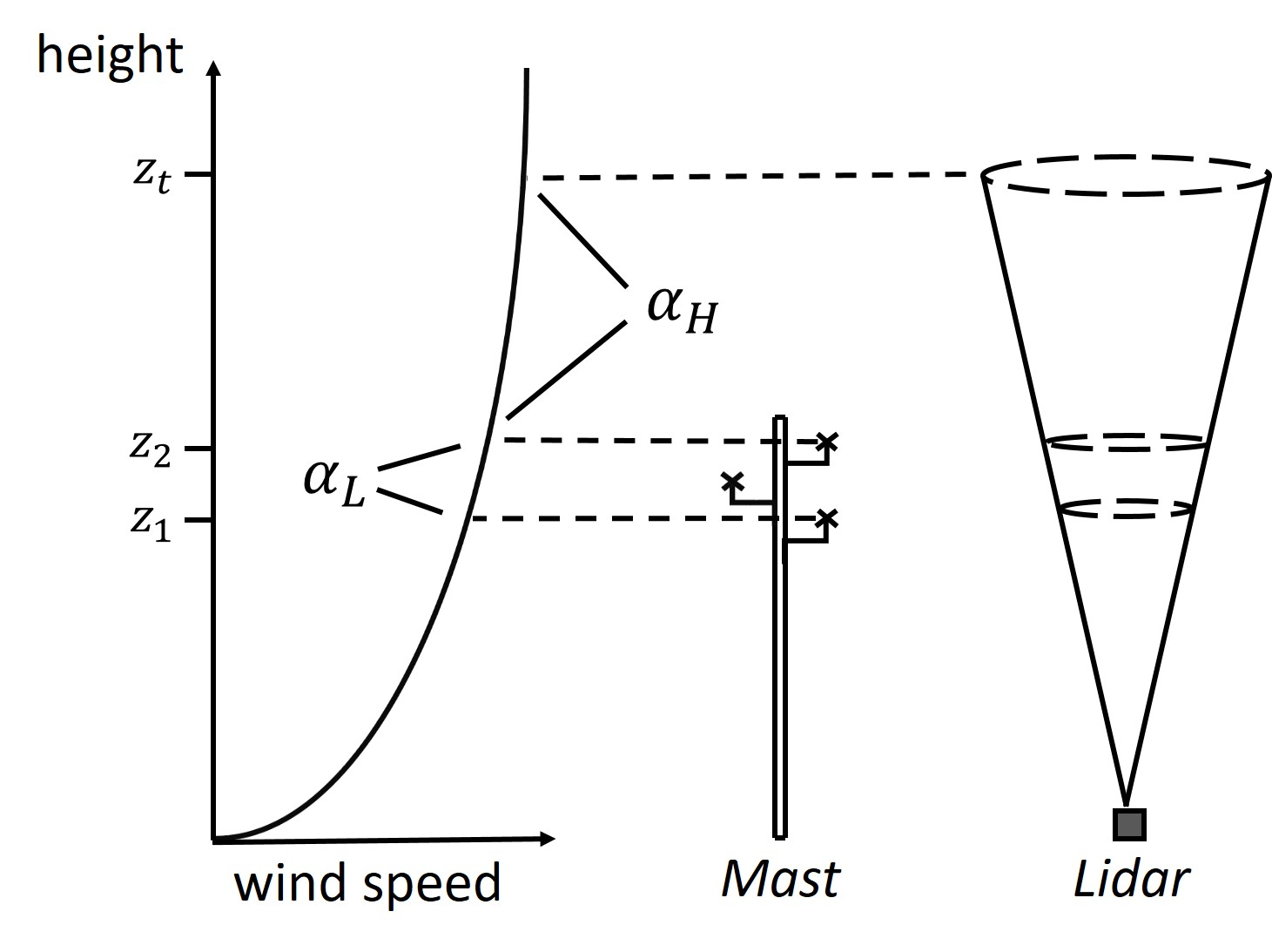
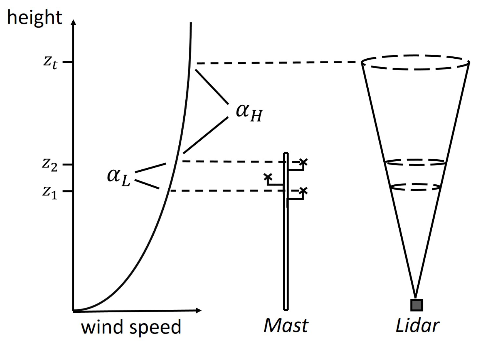
A precise determination of the power law exponent (PLE) is key to accurate wind speed extrapolations. Considering this goal, four different strategies which incorporate the short-term lidar data in the extrapolation process are investigated here. Each of these extrapolation strategies yields a corrected power law exponent α c , which is then used for the extrapolation.
  • Average PLE
    One of the main issues of a mast-based extrapolation using the power law is that the measured α often does not reflect the wind shear above the mast top accurately (i.e., α L α H in Figure 1). When a short-term lidar measurement is carried out next to the mast, the power law exponent in the height range between the mast top and the target height, α H , can be measured directly (see Figure 1). The simplest approach is to derive an average α H from the short-term lidar data and to use it for the extrapolation (i.e., α c = α H ). The mean value of α H is calculated by averaging the 10-min wind speeds within the lidar measurement period and applying Equation (1). The wind shear measured in the height range of the mast is disregarded completely in this extrapolation strategy.
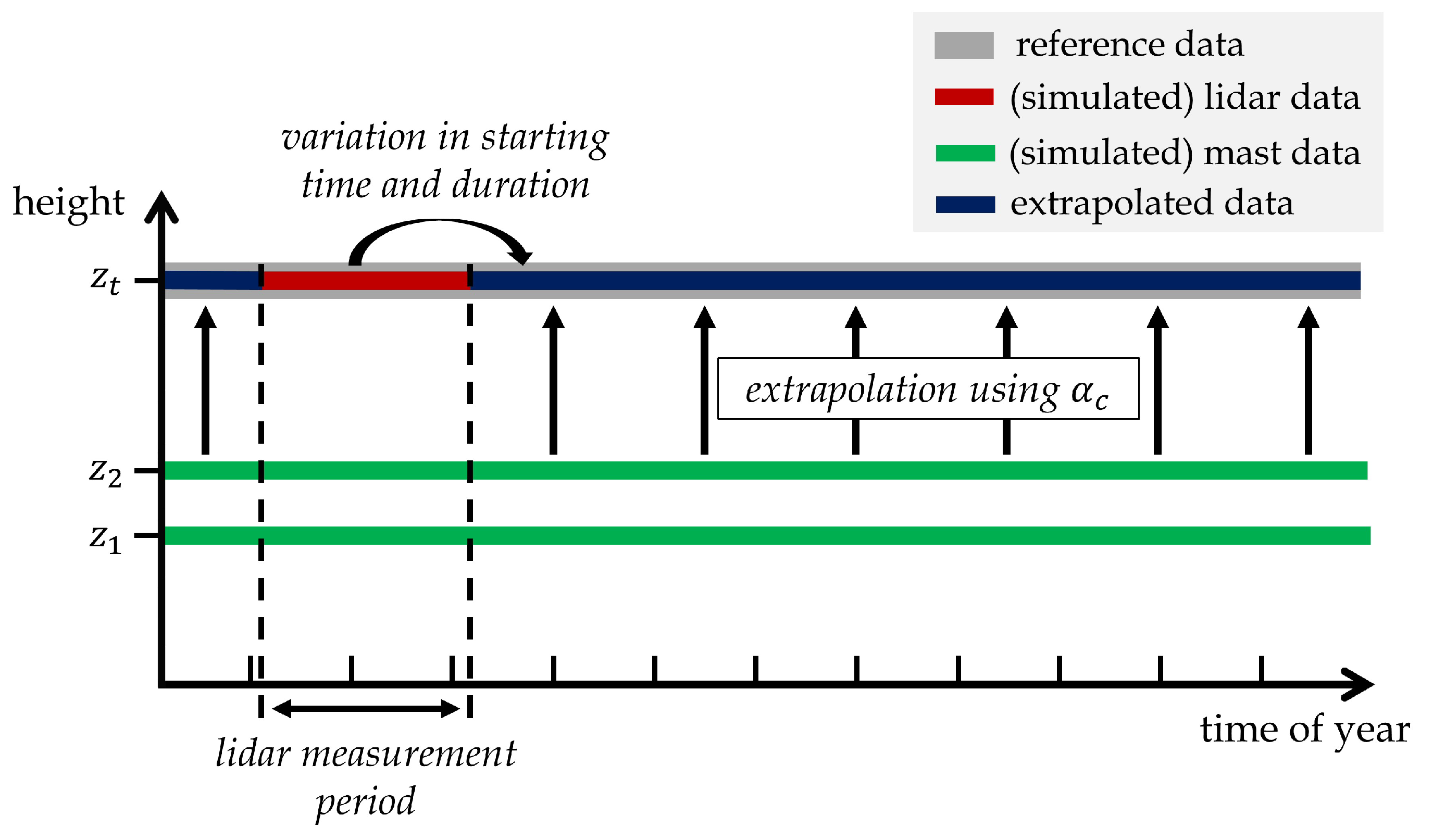
  • Simple Ratio
    The second extrapolation strategy uses a simple relationship between the two power law exponents α H and α L and is based on work published by Lackner et al. [8]. In the simplest case, the relationship can be expressed by the ratio of the mean values of the two power law exponents, R α , determined in the lidar measurement period:
    R α = α H α L
    This relationship is used to adjust the α L value(s) in the period in which no lidar measurement is available and extrapolation has to be conducted (extrapolation period). The corrected power law exponent is then calculated as:
    α c = R α α L
    In contrast to Lackner et al. [8], who extrapolated yearly mean wind speeds, the analysis in this work is based on the extrapolation of ten-min wind speed values. Therefore, the method is adapted on time series in two different ways:
    • Deriving one single α c by applying Equation (3) on the annual mean value of α L . This is equivalent to the method of [8] (delivers the same mean wind speed value) but applied on the time-series values of wind speed.
    • Deriving a time-series of α c values by applying Equation (3) on each time-series value of α L in the extrapolation period. Hence, individual 10-min α c values are used to perform the extrapolation.
    For both cases, R α is calculated using the mean wind profile based on mean wind speeds in the lidar measurement period.
    These methods are named Simple Ratio Mean and Simple Ratio Time-Series (TS) approaches as in 1. one mean α c and in 2. various time-series α c values are derived.
  • Linear Regression
    In a further step, this approach is extended and a linear model is introduced to describe the relationship between α H and α L . An ordinary linear regression of the time-series values of α H and α L (measured during the lidar measurement period) is performed yielding the two regression parameters b 0 and b 1 . In the extrapolation period, the relationship is applied yielding 10-min values of α c :
    α c = b 0 + b 1 α L .
    To ensure a high quality of the linear regression procedure, it is necessary to exclude very high or low values of the correlated parameters. Thus, α L and α H values were excluded from the calculation of b 0 and b 1 which were below (or above) the lowest (or highest) 5% of the α L values measured during the whole year at the respective site.
  • Classification Approach
    As will be shown in Section 4.2, R α varies in time and can not be considered as a constant parameter. In the fourth approach, therefore, additional climatological variables are included in the extrapolation process which are expected to correlate with the temporal variation of R α . This is done by binning the measurement data with respect to atmospheric variables which are measured on site. Within each bin, one set of b 0 and b 1 is derived. In the extrapolation period, the values of b 0 and b 1 are chosen according to the respective value of the classification variable at the corresponding timestamp. Hence, a classified linear regression is performed.
    As for the Linear Regression approach, α L and α H values which were below (or above) the lowest (or highest) 5% of the α L values measured during the whole year were excluded from calculating the values of b 0 and b 1 in the respective bins.
When a time-series based extrapolation with a temporal resolution of 10 minutes is performed, very high (or low) power law exponents can occur. This occurs mainly in case of small wind speeds at one of the heights used in Equation (1). These values do not necessarily represent erroneous measurement data but can bias the extrapolation result. Due to the exponential structure of the power law, this aspect is especially momentous for very high values of the power law exponent. Therefore, values exceeding the 98% quantile of the measured α L at each site were set to the 98% quantile value before performing the extrapolation. This threshold was applied for every extrapolation process guaranteeing the comparability of the results.

3.3. Selection of Classification Variables and Classification Procedure

For the extrapolation based on the Classification Approach, a classification variable needs to be defined. This parameter has to be available during the whole measurement campaign and therefore cannot be part of the lidar measurement only. A homogeneous distribution throughout the year is advantageous. Moreover, its availability from standard measurements in the wind energy community is also desirable.
From a physical perspective, several factors influence the shape of the wind profile. One of the main reasons for temporal variations in wind shear are changes in atmospheric stability. Unfortunately, measurements of atmospheric stability were not available at the sites investigated in this study. In addition, it is usually not measured in resource assessments for wind energy applications. Therefore, atmospheric stability is not considered as a classification variable here.
Temperature obviously has a strong seasonal and diurnal cycle. Additionally, it is closely related to atmospheric stability. However, temperature has the disadvantage that it is distributed very inhomogeneously throughout the year in most regions which limits the applicability. Therefore, additionally to temperature, the relative deviation of each temperature value from the respective daily mean (“relative temperature”) is used in this study.
Wind speed is known to be connected to atmospheric stability [22] and is selected as a classification variable.
Besides atmospheric stability, further important factors influencing the wind profile are surface roughness and orography [7,10,11,23,24]. In a heterogeneous landscape, the wind direction is strongly correlated with the roughness and orography in the upstream fetch and is therefore selected as a classification variable.
Turbulence usually has a strong relation to wind shear. For this reason, both turbulence and standard deviation of the horizontal wind speed provide classification variables. It is noted that vertical profiling wind lidars are known to not measure the standard deviation of wind speed accurately when compared to cup or sonic measurements [25,26]. In this study, however, the standard deviation of the wind speed is only used as a classification variable and, while present, these errors are expected to be of minor importance.
Finally, relative humidity, air density, and air pressure (near the surface) are tested as they often show a good correlation with different meteorological situations.
For the sake of simplicity, the analysis in this paper is restricted to one single classification variable, although it is noted that the classification could also be based on multiple variables concurrently.
The classification in this study is based on dividing the data homogeneously into six classes. Initially, the two outer class bins are determined as containing the lowest or highest 5% of the one-year data of the classification variable. Afterwards, four additional classes are defined in between these bins equidistantly. In the case of classification according to wind direction, six 60-degree sectors were chosen.
To guarantee a sufficient basis for deriving reliable correction factors, a minimum amount of 144 values in each bin was defined, implying that at least one full day of measurement data are available. This value is based on considerations in the guide on wind measurements of the International Electrotechnical Comission [27] where an amount of 144 10-min values is recommended when, e.g., a linear regression is performed for different wind direction bins. While in [27] wind speeds from different locations are correlated, the procedure in this study is applied on power law exponents from different height ranges.
Whenever less than 144 values are detected in one bin, the respective values ( b 0 , b 1 ) are calculated by using the data from all bins. This is equivalent to simply using the parameters of the Linear Regression approach.

3.4. Statistical Analysis and Definition of Error Scores

The (simulated) short-term lidar measurements start every odd day of the year running through the measurement data. This yields more than 180 different, homogeneously separated starting dates. The measurement duration is varied from only a few days up to half a year. Therefore, both the sensitivity of the results to the lidar measurement duration as well as seasonality can be analyzed.
Each time, a time series at the target height is generated by using the measurement data at the target height during the short-term lidar measurement period and extending it with the extrapolated data from the respective extrapolation strategy (see Figure 2). The resulting one-year time series is then compared to the measured wind speeds at the target height (reference data) using the following metrics:
  • Error in (annual) mean wind speed
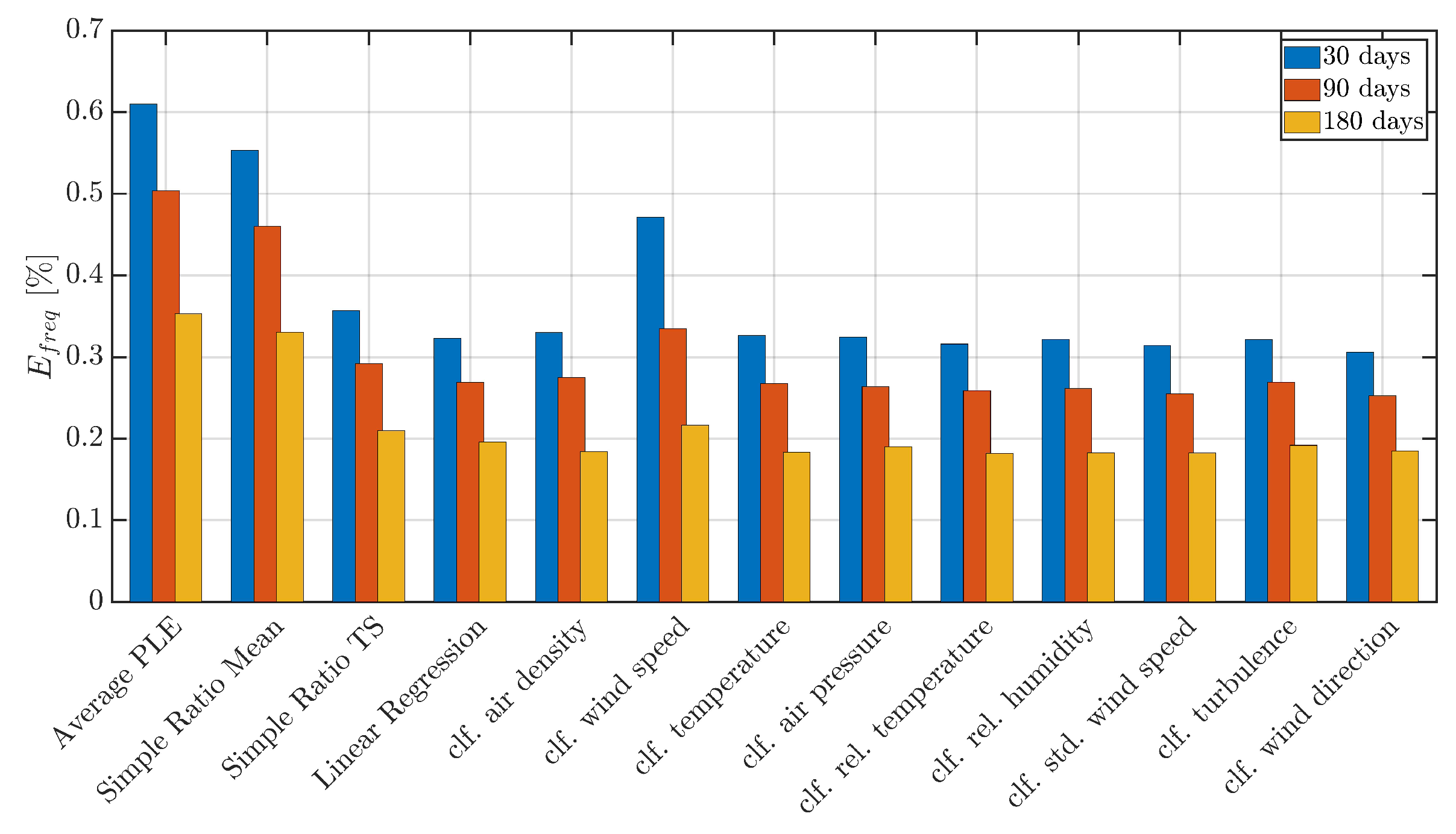
 E m e a n
  • Error in frequency distribution E f r e q
    The wind speed data are divided into bins ranging from 0 to 20 m/s (bin width of 1 m/s, with an additional bin containing all values larger than 20 m/s). The relative frequency of the assessed wind speed values in each bin is compared to the relative frequency of the reference data. Averaging over the deviations using the root mean square error (RMSE) yields the error score E f r e q .
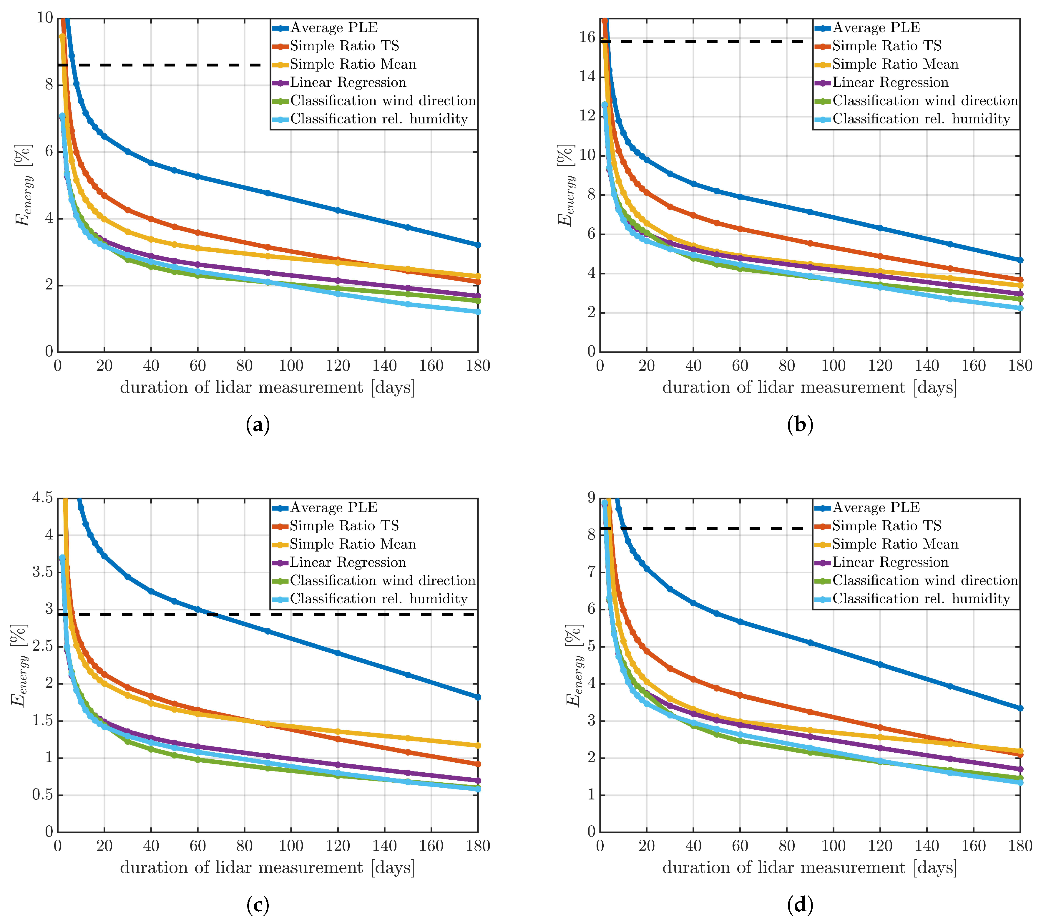
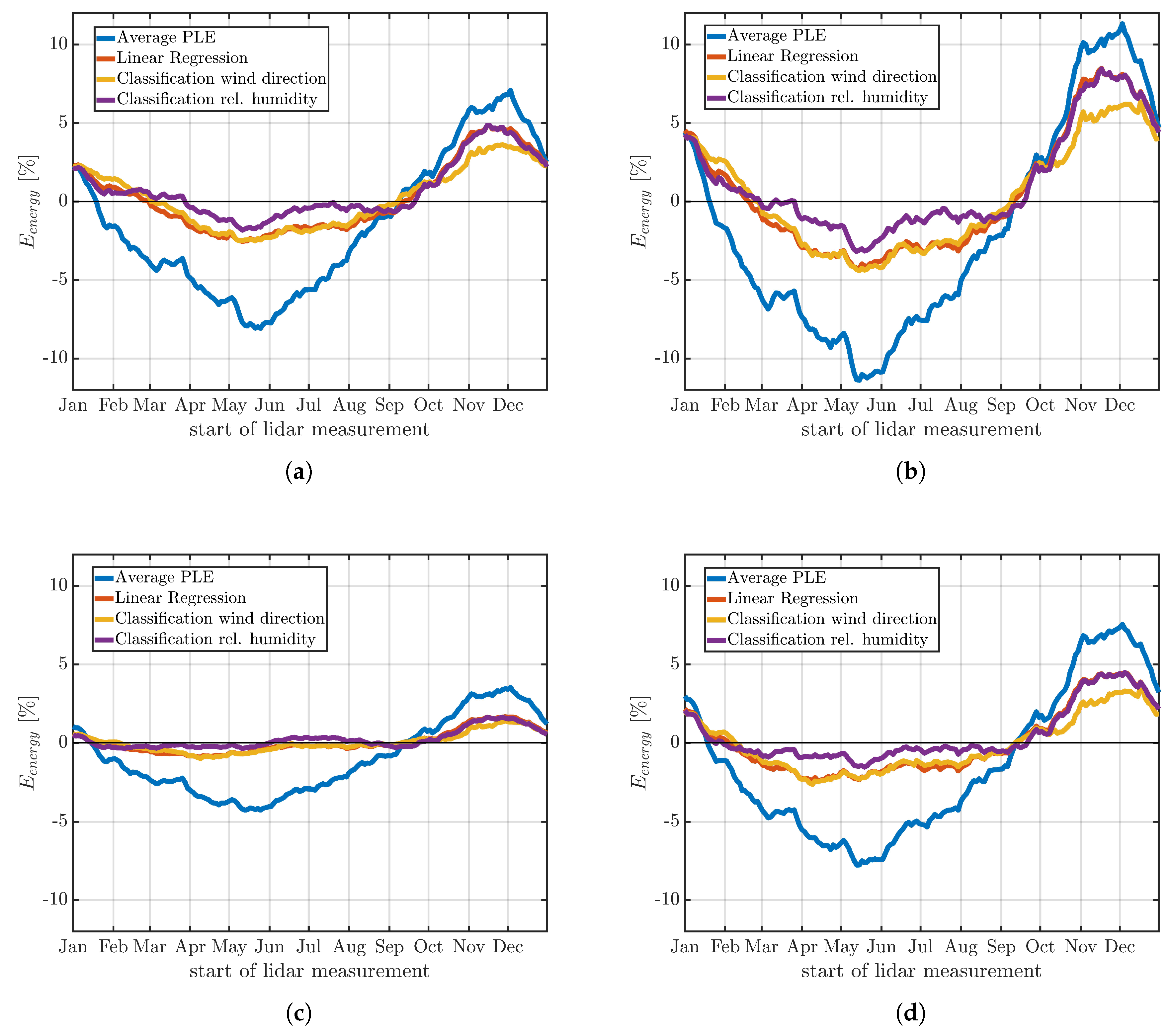
  • Error in the theoretical energy production of a wind turbine E e n e r g y
    The third error score is based on the theoretical energy output of a wind turbine. A power curve of a 3.2 MW wind turbine (see [28]) is used to calculate the (theoretical) one-year energy output from the extrapolated and the reference wind speed time series at the target site. This power curve has a cut-in wind speed at 2 m/s and reaches the nominal power at 14 m/s. At wind speeds of more than 25 m/s, no energy is converted (cut-out wind speed). The energy values related to extrapolated and reference data are then compared (relative deviation) resulting in the error score E e n e r g y .
This procedure is carried out independently for all measurement periods and all measurement sites. After that, an average value of these single extrapolation errors related to one lidar measurement duration is calculated. This yields the overall accuracy of each of the different extrapolation strategies averaged over all sites. In general, the RMSE is used here to calculate the average error value. In order to investigate the effects of seasonality (see Section 4.4.2), however, this is done using the arithmetic mean.
In some cases, the results are compared to the respective extrapolation accuracy when using only met mast data. In this benchmark scenario, the time-series values of α L are used for the vertical extrapolation (applying the 98% threshold criterion described in Section 3.2).

4. Results and Discussion

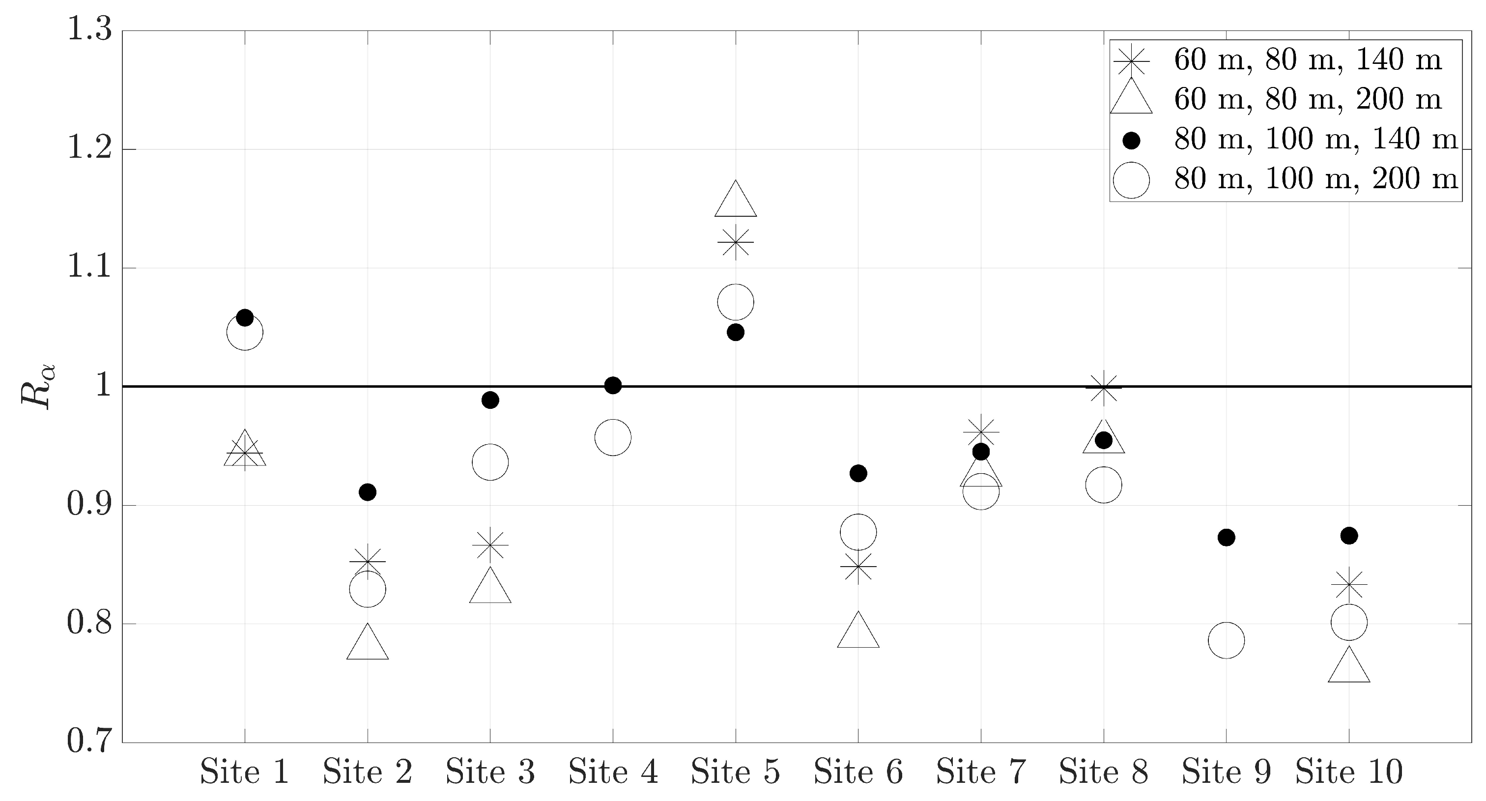
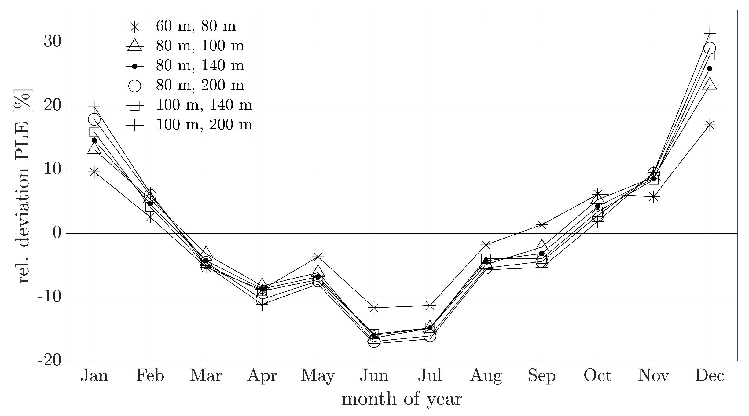
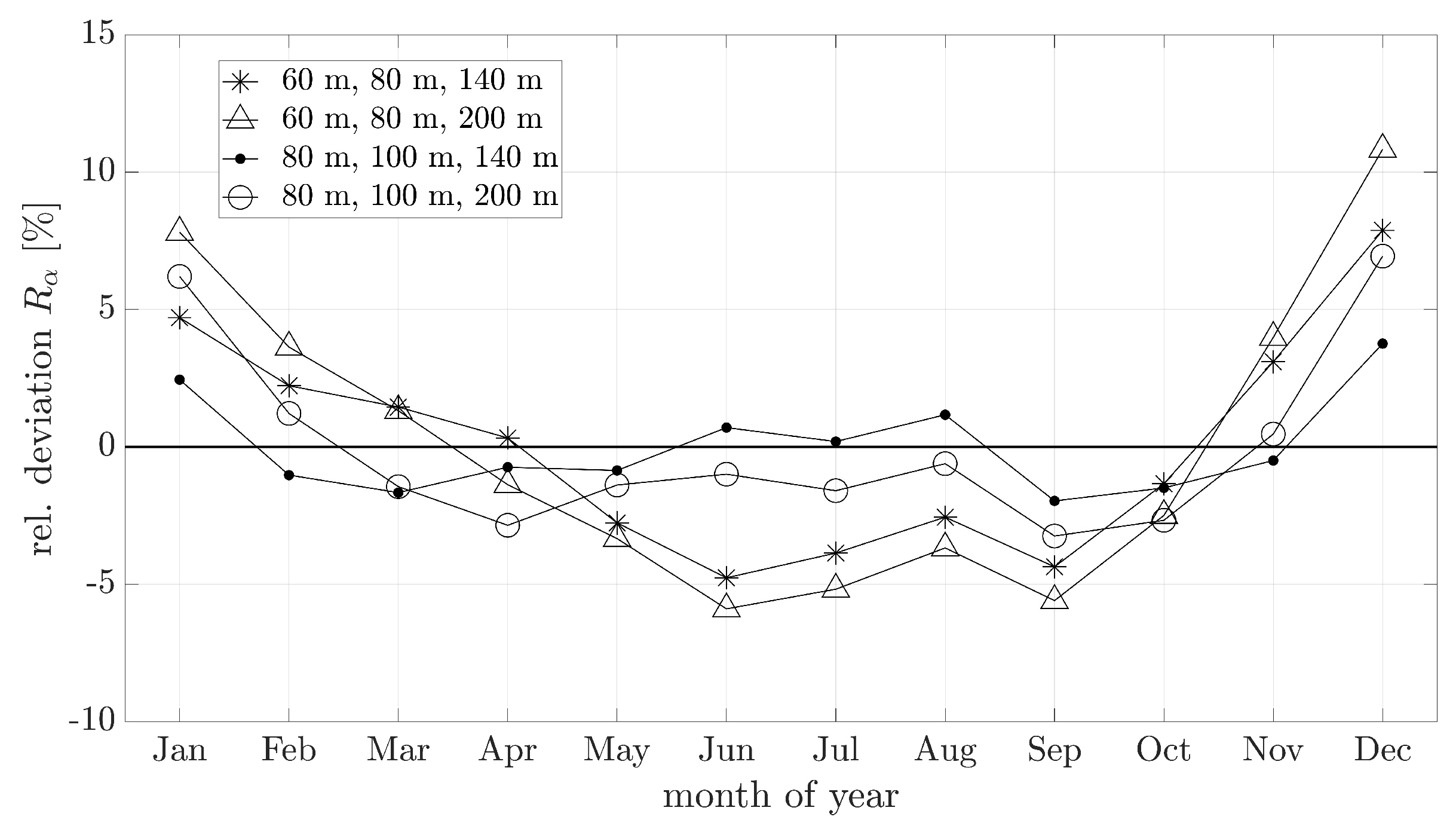
4.1. Height Dependence of the Power Law Exponent

Besides its function in the extrapolation, R α provides a good measure to analyze patterns in wind shear with height and time. R α , calculated from the (annual) mean wind profiles at each site is shown in Figure 3.
In many cases, R α differs significantly from the value of 1 confirming a strong variation of α with height. In general, this is most pronounced for large distances from mast to target height. Furthermore, R α varies strongly from site to site indicating a dependency on site-related properties.
For most sites and height combinations, R α is below 1 representing a decrease of the power law exponent with height. This is in line with the theoretical considerations in [7] and indicates a systematic overestimation of the wind shear when using a measured α L and Equation (1) for the vertical extrapolation of wind speed. However, in some cases, an increase can be identified. This phenomenon was also found in other studies (e.g., [8,11]).
In general, a strongly height-changing power law exponent (represented by high or low R α values) inevitably leads to high extrapolation errors when α L is used for the extrapolation. An overestimation of the wind shear ( R α < 1) directly leads to an overestimation in the extrapolated wind speed. The opposite is the case if α increases with height and the power law exponent in the height range of the mast is smaller than the “true” wind shear above the mast top ( R α > 1). For large extrapolation distances (e.g., extrapolating from 80 to 200 m), the power law exponent measured in the height range of the mast, or the power law in general, can hardly be seen to be suitable and high extrapolation errors can be expected.

4.2. Seasonal Variations of the Wind Profile

Figure 4 depicts the relative seasonal deviation of α from its annual mean. In summer, smaller α values are observed, while winter is characterized by larger shears. The main reason for this behavior is the changing atmospheric stability regime. In Central Europe (the region under investigation in this paper), summers are usually characterized by a higher occurrence of unstable conditions, while in winter stable conditions are more frequent. In their analysis of wind shear in Cabauw, Gualtieri et al. [13] did not find such a clear seasonal pattern in α . However, they only analyzed data for significantly lower heights. More similar results to Figure 4 were obtained by, e.g., [16,29]. The height dependence of the seasonality is rather small for the investigated height range.
While several studies have investigated the seasonal variations of wind shear [10,11,13,16,29,30], the authors are not aware of systematic evaluations of changes in seasonal patterns of α with the height range considered—i.e., the seasonality of R α . Figure 5 shows monthly R α values for different height combinations.
The observed pattern is similar to the pattern in α (Figure 4), especially the winter months are characterized by a high deviation from the yearly mean. The fact that the seasonal cycle of the power law exponent is more pronounced for α H than it is for α L generally results in lower R α values in summer than in winter. The magnitude of the seasonal variation strongly depends on the height combination considered. Interestingly, the values related to the heights above 80 m form a plateau in the summer months. This fact can probably be explained by stronger mixing of the winds of the different layers due to more unstable stratification. The effect of converging wind conditions, as mentioned above, appears to be more pronounced at higher altitudes. Note that at two sites no measurement data were available at the 60 m level which may somehow restrict the comparability. The seasonal patterns as observed in Figure 5, however, are not affected by this.

4.3. Extrapolation Errors in Wind Speed

Figure 6 shows E m e a n for a short, a medium, and a long lidar measurement period (30, 90, and 180 days). Mast and target height are set to z 2 = 80 m and z t = 140 m . Results for other height combinations are very similar. Compared to the average extrapolation error using only the met mast data (3.79%), all extrapolation methods incorporating the short-term lidar data yield a significant improvement.
As expected, E m e a n decreases with increasing lidar measurement duration for all extrapolation strategies. On the one hand, this is due to more data which increases the representativity of the measurement and ensures higher reliability of the derived parameters (i.e., α H , R α , b 0 , and b 1 ). On the other hand, the wind speed at the target height is measured directly over a longer period. For this period, no extrapolation is necessary (see Figure 2). This automatically reduces the error.
Clearly, in comparison to the other extrapolation strategies, the Average PLE approach delivers the worst results. On average, however, it still yields better results than extrapolating without additional lidar data (i.e., using only mast data) even after a lidar measurement duration of 30 days.
In case of very short lidar measurement periods, the Simple Ratio Mean approach delivers the most accurate mean wind speeds. The respective error, however, does not decrease appreciably when the lidar measurement is extended. Thus, for the long lidar measurement (180 days), the Simple Ratio Time-Series, the Linear Regression, and the Classification approaches all yield better results. The best results for a measurement period of 180 days are achieved by a classification according to relative humidity. Moreover, a classification according to relative or absolute temperature, air density, or wind direction yields comparable results.
These results indicate that, in case of very short lidar measurement periods, a classification does not improve the estimation of the mean wind speed compared to the non-classified Linear Regression or Simple Ratio Mean approaches. This can be explained by the fact that only a small amount of data are available which makes the calculations in the classification scheme less reliable.
Figure 7 shows the error in the frequency distribution of wind speed, E f r e q . E f r e q amounts to 0.56% when no short-term lidar data are used (extrapolating using only mast data). As for E m e a n , the Average PLE method shows the worst performance. The analysis also reveals that the Simple Ratio Mean approach cannot reproduce the frequency distribution accurately despite its high accuracy in mean wind speed. The Simple Ratio Time-Series, the Linear Regression as well as the Classification approaches yield more accurate frequency distributions. Interestingly, all these methods are based on using time series of α c . This stresses the importance of considering the temporal variability of the wind profile for the height-dependent wind speed distribution. In practical applications, this aspect is often neglected. The time-series based extrapolation methods, introduced in this paper, directly address this phenomenon. At the same time, they avoid the problems of deriving general models for the height-dependent shape of wind speed distributions above the surface layer (as reported by, e.g., [31]) and in complex terrain. A comparison of the different methods reveal that, on average, slight improvements are achieved when the classification procedure (e.g., for wind direction) is integrated in the linear regression process.

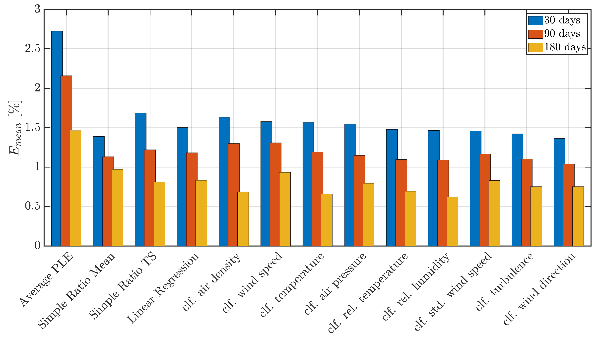
4.4. Extrapolation Errors in Energy Yield

4.4.1. Dependence on Lidar Measurement Duration

In Figure 8, the results for E e n e r g y are presented in more detail for selected extrapolation strategies. Here, the E e n e r g y values are shown for all the different combinations of mast and target height investigated in this study. As expected, E e n e r g y is significantly higher for larger height ranges.
Again, the Average PLE approach generally shows itself to be the most inaccurate way to integrate the lidar data into the extrapolation process. This can be found for all the investigated height combinations according to Figure 8. For short height ranges (Figure 8c), this procedure even increases the error compared to an extrapolation using only met mast data when the lidar measurement is carried out over less than two months.
In contrast, the Linear Regression method performs significantly better. Binning the data with respect to wind direction or relative humidity (Classification approach) further improves the extrapolation accuracy. This is particularly pronounced for long lidar measurement periods when a larger amount of data are collected and a solid calculation of the parameters of linear regression within each bin is possible.
Both Simple Ratio approaches tested in this study show worse performance compared to the methods based on linear regression. The probable reasons for this are that, while Simple Ratio Mean cannot deliver an accurate wind speed distribution, the Simple Ratio Time-Series approach has a smaller accuracy regarding the mean wind speed. Similar to the results for the mean wind speed (see Figure 6), the Simple Ratio Mean method performs better for short measurement periods, while the Simple Ratio Time-Series performs better for longer measurement periods (for three out of four investigated height combinations).
When compared to the extrapolation using only met mast data, the extrapolation accuracy generally is increased significantly already after a lidar measurement period of only a few days. When the lidar measurement is carried out over a period of one to two months, the extrapolation error can be reduced by more than 60% on average. A further increase of the lidar measurement period only slightly reduces the error.

4.4.2. Seasonality

In a next step, dependencies of the extrapolation accuracy with respect to the temporal position of the lidar measurement in the year are investigated. Due to their good performance in extrapolating wind speed and energy yield (Section 4.3 and Section 4.4.1), the analysis is limited to the Linear Regression and the Classification (relative humidity and wind direction) approaches. As a baseline comparison, the Average PLE approach is also shown. The seasonal course of E e n e r g y (arithmetic mean over all sites) is shown in Figure 9. The lidar measurement duration is set to an exemplary duration of 60 days. (Increasing the lidar measurement duration flattens the lines and decreases the amplitudes but does not change the essential conclusions discussed below.) Figure 9 therefore gives an impression on systematic biases connected to seasonal aspects of the wind climate.
The seasonal patterns observed in E e n e r g y resemble those in Figure 4 and Figure 5. In summer, generally smaller α and R α values occur while in winter higher values are more frequent. As discussed, this is likely due to seasonal variations in atmospheric stability conditions. These aspects directly result in large underestimations of the Average PLE approach when the lidar measurement is performed in summer and large overestimations when the lidar measurement is carried out in winter periods. Applying the Linear Regression method significantly decreases the seasonal biases. When a classification according to relative humidity is applied, the systematic “summer bias” can be decreased further while a classification according to wind direction allows for achieving slightly more accurate results when the lidar measurement is carried out in winter.
To the authors’ knowledge, relative humidity is generally not known for having a significant influence on the wind profile. Instead, relative humidity as an environmental variable can probably rather be considered to reflect other variables (mainly atmospheric stability), which, in turn, influence the wind profile. Heating and cooling of the air reduces or increases the value of relative humidity. Hence, the relative humidity of the air varies similarly to atmospheric stability, with solar radiation.
At the measurement sites investigated in this study, a substantial variation in relative humidity can only be detected in spring or summer months. In fall or winter, however, almost only high relative humidity values occur. As a consequence, for most classification bins, only a relatively small amount of values is then available to calculate b 0 and b 1 . This is the likely reason that no improvement is achieved compared to the non-classified Linear Regression approach when the lidar measurement is set to a winter period.
While for all extrapolation strategies some seasonality remains, the systematic biases can be reduced when the Classification approach is used.

5. Conclusions

It was shown that the accuracy in the vertical extrapolation of wind speed can be increased significantly when short-term lidar measurements at the target height are used. Lidar measurements with a duration of only a few weeks already yielded very good results.
In this context, the power law exponent (serving as a quantity describing the wind shear) was analyzed, revealing a strong variation of the power law exponent from site to site as well as a strong height dependence. In particular, the latter aspect leads to high extrapolation errors when the mast measurement is extrapolated over a large height range and underlines the need for advanced extrapolation procedures. Carrying out an additional lidar measurement is one possibility to face this issue. As could be shown, the methodology of incorporating the lidar data into the extrapolation process is decisive in this context. A simple ratio approach proved to deliver very accurate mean wind speeds. Larger errors, however, occurred in determining the frequency distribution of wind speed or the theoretical energy production of a wind turbine. A linear regression procedure proved to yield the highest extrapolation accuracies in general. Binning the data with respect to certain meteorological conditions further increased the extrapolation accuracy as seasonal biases, connected to the temporal position of the lidar measurement in the year, could be decreased. Wind direction and, unexpectedly, relative humidity served as advantageous classification variables here.
All in all, lidar measurement periods of only one to two months proved to be sufficient to decrease the extrapolation error in (theoretical) energy yield by around 50% to 70% on average. The effect is especially momentous for large extrapolation height ranges. Hence, the presented extrapolation strategies deliver a possibility to decrease the extrapolation error even for large extrapolation ranges on a level that can be seen acceptable in wind resource assessment. This can be seen to be especially momentous when considering future trends in the wind energy industry as turbine heights are expected to continue to increase.

Author Contributions

A.B. had the lead in writing the manuscript and developing the methodology for this study. A.B. also performed all data analysis and visualization. L.P. developed the initial concept for the design of the analysis, initiated the study, and contributed to writing several sections of the article. L.P. and D.C. had a supervisory role during the development of the methodology, data analysis, and the writing process. All authors revised and edited the manuscript. D.C. was also responsible for the funding acquisition and the project administration. All authors have read and agreed to the published version of the manuscript.

Funding

This research was funded by the Federal Ministry of Economic Affairs and Energy (Bundesministerium für Wirtschaft und Energie, BMWi) on the basis of a decision by the German Bundestag, Grant No.: 0324159E.

Acknowledgments

We thank GWU Umwelttechnik GmbH, Notus Energy, and NES GmbH for providing measurement data.

Conflicts of Interest

The authors declare no conflict of interest.

Abbreviations

The following abbreviations are used in this manuscript:
AEPAnnual Energy Production (of a wind turbine)
PLEPower Law Exponent
RMSERoot Mean Square Error
TSTime Series

References

  1. Rohrig, K.; Berkhout, V.; Callies, D.; Durstewitz, M.; Faulstich, S.; Hahn, B.; Jung, M.; Pauscher, L.; Seibel, A.; Shan, M.; et al. Powering the 21st century by wind energy—Options, facts, figures. Appl. Phys. Rev. 2019, 6, 031303. [Google Scholar] [CrossRef]
  2. Prandtl, L. Meteorologische Anwendung der Strömungslehre. Beitr. Phys. Atmos. 1932, 19, 188–202. [Google Scholar]
  3. Obukhov, A.M. Turbulence in an atmosphere with a non-uniform temperature. Bound.-Layer Meteorol. 1971, 2, 7–29. [Google Scholar] [CrossRef]
  4. Foken, T. 50 Years of the Monin–Obukhov Similarity Theory. Bound.-Layer Meteorol. 2006, 119, 431–447. [Google Scholar] [CrossRef]
  5. Gryning, S.E.; Batchvarova, E.; Brümmer, B.; Jørgensen, H.; Larsen, S. On the extension of the wind profile over homogeneous terrain beyond the surface boundary layer. Bound.-Layer Meteorol. 2007, 124, 251–268. [Google Scholar] [CrossRef]
  6. Hellmann, G. Über die Bewegung der Luft in den untersten Schichten der Atmosphäre; Königlich Preußische Akademie der Wissenschaften zu Berlin: Berlin, Germany, 1914. [Google Scholar]
  7. Emeis, S. Wind Energy Meteorology: Atmospheric Physics for Wind Power Generation; Springer: Berlin/Heidelberg, Germany, 2013. [Google Scholar]
  8. Lackner, M.A.; Rogers, A.L.; Manwell, J.F.; McGowan, J.G. A new method for improved hub height mean wind speed estimates using short-term hub height data. Renew. Energy 2010, 35, 2340–2347. [Google Scholar] [CrossRef]
  9. Gualtieri, G. A comprehensive review on wind resource extrapolation models applied in wind energy. Renew. Sustain. Energy Rev. 2019, 102, 215–233. [Google Scholar] [CrossRef]
  10. Hanafusa, T.; Lee, C.B.; Lo, A.K. Dependence of the exponent in power law profiles on stability and height interval: Short Communication. Atmos. Environ. 1986, 20, 2059–2066. [Google Scholar] [CrossRef]
  11. Li, J.; Wang, X.; Yu, X. Use of spatio-temporal calibrated wind shear model to improve accuracy of wind resource assessment. Appl. Energy 2018, 213, 469–485. [Google Scholar] [CrossRef]
  12. Touma, J.S. Dependence of the Wind Profile Power Law on Stability for Various Locations. J. Air Pollut. Control Assoc. 1977, 27, 863–866. [Google Scholar] [CrossRef]
  13. Gualtieri, G. Atmospheric stability varying wind shear coefficients to improve wind resource extrapolation: A temporal analysis. Renew. Energy 2016, 87 Pt 1, 376–390. [Google Scholar] [CrossRef]
  14. Irwin, J.S. A theoretical variation of the wind profile power-law exponent as a function of surface roughness and stability: Technical Note. Atmos. Environ. 1979, 13, 191–194. [Google Scholar] [CrossRef]
  15. Hussain, M. Dependence of power law index on surface wind speed. Energy Convers. Manag. 2001, 43, 467–472. [Google Scholar] [CrossRef]
  16. Pérez, I.A.; García, M.A.; Sánchez, M.L.; de Torre, B. Analysis and parameterisation of wind profiles in the low atmosphere. Sol. Energy 2005, 78, 809–821. [Google Scholar] [CrossRef]
  17. Pauliac, R. WINDCUBE User’s Manual, Orsay; Leosphere: Saclay, France, 2009. [Google Scholar]
  18. Emeis, S.; Harris, M.; Banta, R.M. Boundary-layer anemometry by optical remote sensing for wind energy applications. Meteorol. Z. 2007, 16, 337–347. [Google Scholar] [CrossRef] [Green Version]
  19. Elkinton, M.R.; Rogers, A.L.; McGowan, J.G. An Investigation of Wind-Shear Models and Experimental Data Trends for Different Terrains. Wind Eng. 2006, 30, 341–350. [Google Scholar] [CrossRef]
  20. Ray, M.L.; Rogers, A.L.; McGowan, J.G. Analysis of wind shear models and trends in different terrains. Proc. Am. Wind Energy Assoc. Wind. 2006. Available online: http://citeseerx.ist.psu.edu/viewdoc/download?doi=10.1.1.574.7468&rep=rep1&type=pdf (accessed on 20 January 2020).
  21. Leleu, K. Leosphere Windcube User Guide, Version V.1.2 (March 2019); Leosphere: Saclay, France, 2019. [Google Scholar]
  22. Blackadar, A.K. Turbulence and Diffusion in the Atmosphere; Springer: Berlin/Heidelberg, Germnay, 1997. [Google Scholar]
  23. Bechrakis, D.A.; Sparis, P.D. Simulation of the Wind Speed at Different Heights Using Artificial Neural Networks. Wind Eng. 2000, 24, 127–136. [Google Scholar] [CrossRef]
  24. Emeis, S. Vertical variation of frequency distributions of wind speed in and above the surface layer observed by sodar. Meteorol. Z. 2001, 10, 141–149. [Google Scholar] [CrossRef]
  25. Pauscher, L.; Klaas, T.; Callies, D.; Foken, T. Wind obsevations from a forested hill: Relating turbulence statistics to surface characteristics in hilly and patchy terrain. Meteorologische Zeitschrift 2017. submitted. [Google Scholar]
  26. Sathe, A.; Mann, J.; Gottschall, J.; Courtney, M.S. Can Wind Lidars Measure Turbulence? J. Atmos. Ocean. Technol. 2011, 28, 853–868. [Google Scholar] [CrossRef] [Green Version]
  27. IEC. IEC 61400-12 Wind Turbines—Part 12-1: Power Performance Measurements of Electricity Producing Wind Turbines Draft FDIS 2nd ed. 2016. Available online: https://webstore.iec.ch/publication/26603 (accessed on 20 January 2020).
  28. Website Enercon: Overview of Technical Details on E-115. Available online: https://www.enercon.de/en/products/ep-3/e-115/ (accessed on 1 August 2019).
  29. Farrugia, R.N. The wind shear exponent in a Mediterranean island climate. Renew. Energy 2002, 28, 647–653. [Google Scholar] [CrossRef]
  30. Rehman, S.; Al-Abbadi, N.M. Wind shear coefficients and their effect on energy production. Energy Convers. Manag. 2005, 46, 2578–2591. [Google Scholar] [CrossRef]
  31. Kelly, M.; Troen, I.; Jørgensen, H.E. Weibull-k Revisited: “Tall” Profiles and Height Variation of Wind Statistics. Bound.-Layer Meteorol. 2014, 152, 107–124. [Google Scholar] [CrossRef] [Green Version]
Figure 1. (Theoretical) measurement setup and power law exponents α L in the height range of the mast (i.e., between z 1 and z 2 ) and α H between mast top and target height ( z 2 and z t ), respectively.
Remotesensing 12 01091 g001
Figure 2. Methodology of the selection of the lidar measurement period and extrapolation. α c is derived using the mast data at heights z 1 , z 2 and the lidar data at the target height z t during the lidar measurement period (red). During the extrapolation period, the mast data are extrapolated from z 2 to z t . The extrapolated data (blue) then are merged with the lidar data. Finally, the resulting time series is compared to the reference data at z t (grey).
Remotesensing 12 01091 g002
Figure 3. Height dependence of the power law exponents expressed by using the quantity R α . Shown for four different combinations of z 1 , z 2 and z t using annual mean wind speeds. Note that, at Site 4 and Site 9, no measurement data at the 60 m level were available (see Table 1).
Remotesensing 12 01091 g003
Figure 4. Relative deviation of monthly power law exponents from the yearly mean (based on monthly mean wind speeds), shown for different height ranges. The results from all measurement sites are averaged arithmetically yielding one curve per height combination.
Remotesensing 12 01091 g004
Figure 5. Relative deviation of monthly R α values from the yearly mean (based on monthly mean values of wind speed). Averaged over all sites and shown for different height ranges.
Remotesensing 12 01091 g005
Figure 6. Extrapolation errors E m e a n for z 2 = 80 m , z t = 140 m and varying durations of the lidar measurement; for extrapolation without short-term lidar data, E m e a n = 3.79 % .
Remotesensing 12 01091 g006
Figure 7. Extrapolation errors E f r e q for z 2 = 80 m , z t = 140 m and varying durations of the lidar measurement; for extrapolation without short-term lidar data, E f r e q = 0.56 % .
Remotesensing 12 01091 g007
Figure 8. The average extrapolation error E e n e r g y in dependence of the duration of the lidar measurement (RMSE over all sites and starting times), for (a) z 2 = 80 m and z t = 140 m; (b) z 2 = 80 m and z t = 200 m; (c) z 2 = 100 m and z t = 140 m; (d) z 2 = 100 m and z t = 200 m. The black dashed lines represent the errors of the scenario of extrapolating without lidar data.
Remotesensing 12 01091 g008
Figure 9. The average extrapolation error E e n e r g y for different extrapolation approaches in dependence of the start of the lidar measurement, for (a) z 2 = 80 m and z t = 140 m; (b) z 2 = 80 m and z t = 200 m; (c) z 2 = 100 m and z t = 140 m; (d) z 2 = 100 m and z t = 200 m. Selected lidar measurement duration: 60 days.
Remotesensing 12 01091 g009
Table 1. Details of the measurement sites; d indicates the displacement height estimated as 2/3 of the height of trees near the measurement location (as often done in wind energy applications when performing vertical extrapolation [7,19,20]). The duration of each measurement is exactly one year. The measurements were carried out at different one-year periods between May 2014 and August 2018. At Sites 4 and 9, no measurement data were available at the 60 m level.
SiteOrography and Surface Coverd [m]Measurement Heights [m]Device Used for Measurement
Site 1hilly, forested1860, 80, 100, 140, 200WindCube V2
Site 2slightly hilly, forested1860, 80, 100, 140, 200WindCube V2
Site 3mainly flat, forested1660, 80, 100, 140, 200WindCube V2
Site 4hilly, sparsely forested1280, 100, 140, 200WindCube V1
Site 5slightly hilly, barely forested060, 80, 100, 140, 200WindCube V1
Site 6slightly hilly, forested1660, 80, 100, 140, 200WindCube V2
Site 7hilly, forested1660, 80, 100, 140, 200WindCube V1
Site 8slightly hilly, no trees060, 80, 100, 140, 200WindCube V1
Site 9slightly hilly, sparsely forested1480, 100, 140, 200WindCube V1
Site 10slightly hilly, forested1460, 80, 100, 140, 200WindCube V2

