Site-Adaptation of Modeled Solar Radiation Data: The SiteAdapt Procedure


Abstract
1. Introduction
- the treatment of the effect of clouds in solar radiation attenuation;
- the irradiance modeling under clear sky conditions;
- the area integrated by the satellite pixel leads to inaccuracies mainly during intermittent cloudy weather and changing aerosol load, which is the so-called “nugget effect” [18];
- terrain effects and the high reflective albedo of deserts and snow
2. Materials and Methods
2.1. Solar Radiation Data
2.1.1. Ground Measured Data
- Baseline surface radiation network (BSRN). The BSRN is a project managed under by the World Climate Research Program (WCRP), and imposes high quality standards, both in instrumentation and maintenance. Global horizontal solar irradiation (GHI) and direct normal solar irradiation (DNI) data were used in this work.
- UO SRML: The activity of the solar radiation monitoring laboratory of the University of Oregon started in 1977, with the creation of a five-station global network under the auspices of the Pacific northwest regional commission, motivated by the lack of available and accurate solar radiation data. This network covers the States of Idaho, Montana, Oregon, Utah, Washington and Wyoming, with 39 stations. The data are recorded with an hourly interval before 1995 and of 5 min afterward, and the associated estimated uncertainties for daily irradiances are 2% for DNI and 5% for GHI. The radiometers are calibrated on a yearly basis with periodic on-site checks with reference radiometers.
2.1.2. Modeled Data
- The NSRDB (national solar radiation data base), that provides solar irradiance at a 4-km horizontal resolution for each 30-min interval from 1998 to 2016 over the United States and regions of the surrounding countries [28]. It was computed by the National Renewable Energy Laboratory’s (NREL’s) physical solar model (PSM) and products from the National Oceanic and Atmospheric Administration’s (NOAA’s) geostationary operational environmental satellite (GOES), the National Ice Center’s (NIC’s) interactive multisensor snow and ice-mapping system (IMS) and the National Aeronautics and Space Administration’s (NASA’s) moderate resolution imaging spectroradiometer (MODIS) and modern era retrospective analysis for research and applications, version 2 (MERRA-2).
- The CAMS-RAD database, provided by the atmosphere service of Copernicus, the European program for the establishment of a European capacity for earth observation with respect to land, marine and atmosphere monitoring, emergency management, security and climate change [29]. This database was calculated by means of the Heliosat-4 method [15], a fully physical model using a fast, but still accurate approximation of radiative transfer modeling. It is composed of two models based on abaci, also called lookup tables: the McClear [30] model calculating the irradiance under cloud-free conditions and the McCloud model calculating the extinction of irradiance due to clouds. Both were constructed by using the LibRadtran [31] radiative transfer model. The main inputs to Heliosat-4 are aerosol properties, total column water vapor and ozone content as provided by the CAMS global services every 3 h. Cloud properties are derived from images of the Meteosat Second Generation (MSG) satellites in their 15 min temporal resolution using an adapted APOLLO (AVHRR processing scheme over clouds, land and ocean) scheme.
2.2. The SiteAdapt Procedure
2.2.1. Preprocessing
- GHI preprocessing. It relies on the regression of the measured clearness index (kt, the ratio of GHI to top-of-atmosphere solar irradiance on the same plane) on the best combination of the following variables: α; kt of modeled series; relative air mass (m, based on Kasten formulation [34]); modeled clear-sky index (kc, the ratio between modeled GHI and its corresponding value under clear-sky conditions, calculated through the McClear model [30]).
- DHI preprocessing: it relies on the regression of the ratio DHI to GHI (kd, diffuse ratio) of measured data on the following variables: m; Kc; α; ktm designed to diminish the solar zenith angle dependence of kt by normalizing it with respect to a standard clear-sky GHI profile, normalized to 1 for a relative air mass of 1 [35] Equation (1):
- DNI preprocessing: it is calculated from both preprocessed GHI and DHI by the closure Equation (2):where θ is the solar zenith angle expressed in radians. It was found that using a fourth order polynomial of ktm provides better results than simply using ktm.
2.2.2. Empirical Quantile Mapping (eQM) Correction
2.2.3. Postprocessing
- Extreme values. To determine extremely high values, it was imposed that the maximum annual values measured (and validated) for GHI and DNI are not exceeded by 5% and that the DHI does not exceed 700 W/m2. Negative solar data have were also defined as erroneous data.
2.3. Statistical Indicators
- Class A: relative mean bias difference (relbias); relative mean absolute difference (relMAD); relative root mean square difference (relRMSD). These indicators quantify the dispersion (or “error”) of individual points (their value would be 0 for a perfect model);
- Class C: Kolmogorov–Smirnov test Integral (KSI) and OVER [42]. These indicators quantify the distribution similarity (a lower value indicates better distributions similarity). KSI estimates the area between the CDFs of the datasets to be compared and OVER is also an estimate of the area between the CDFs, but only for the parts where a critical value distance is exceeded.
2.4. Case Study
3. Results
3.1. Preprocessing
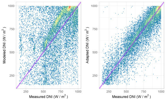
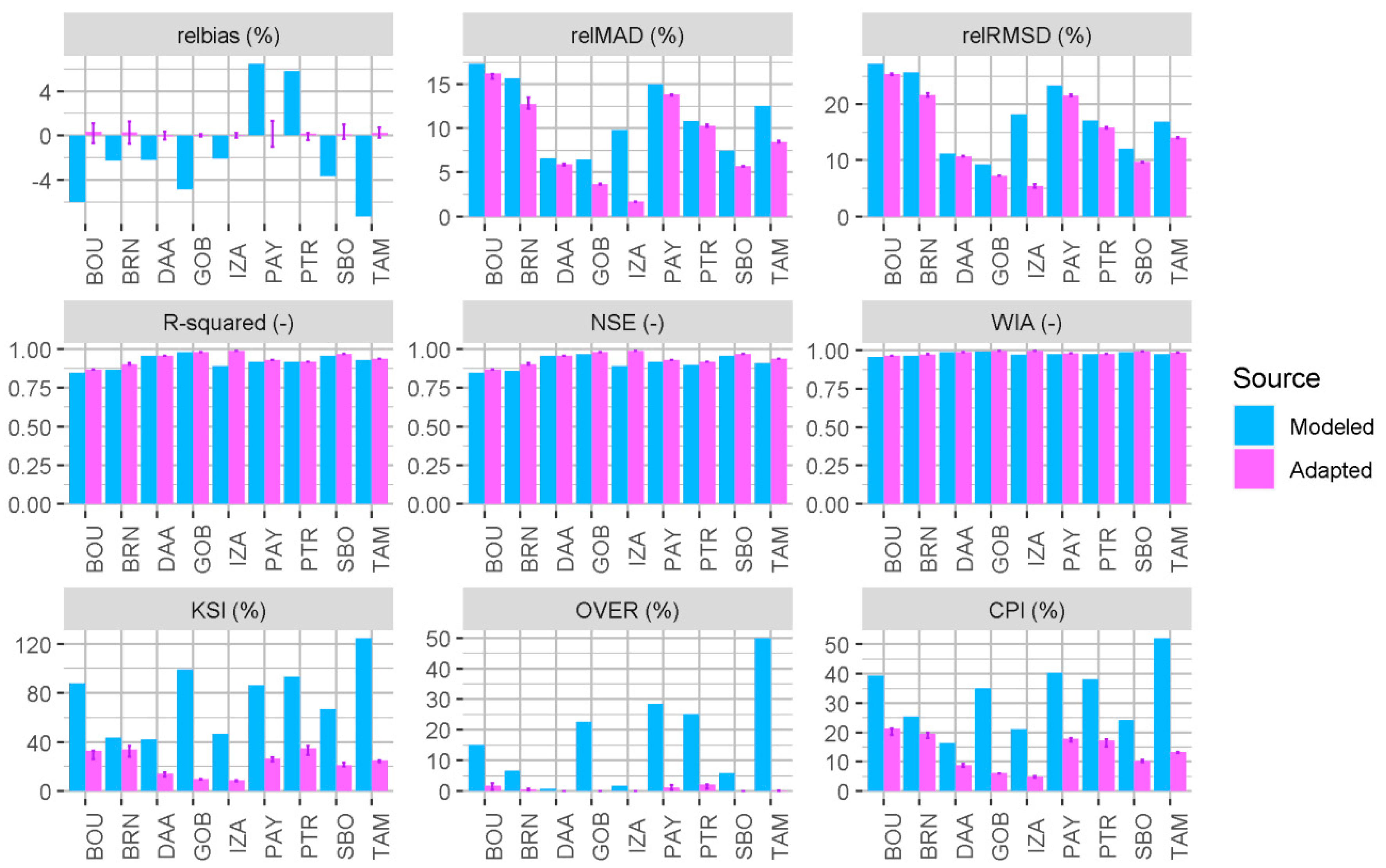
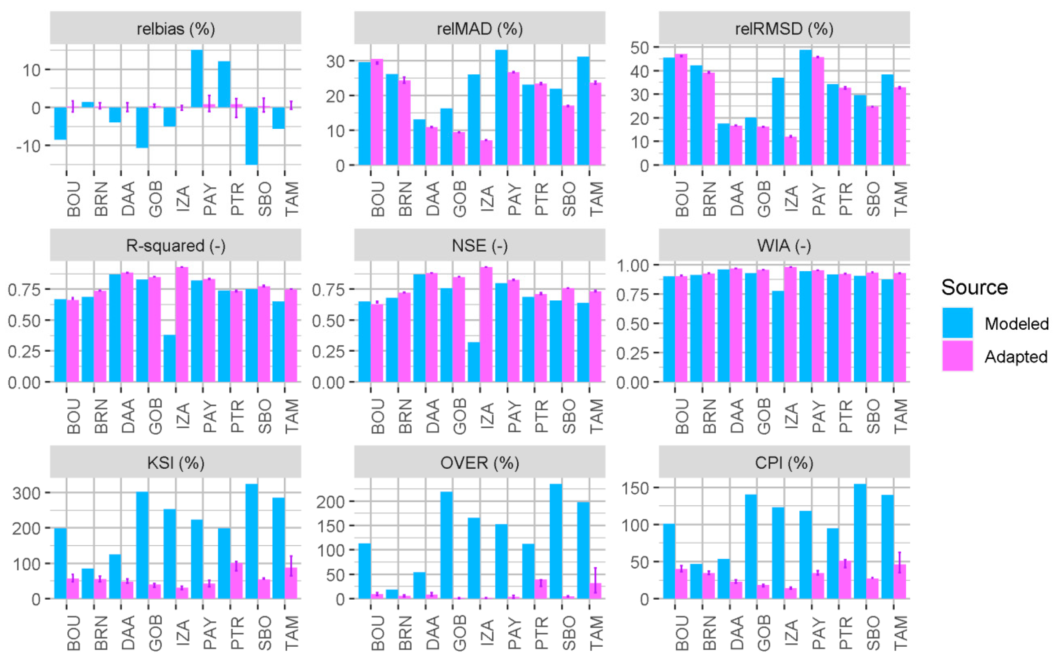
3.2. Site-Adaptation Performance
3.3. Prediction of Site-Adaptation Performance
4. Discussion
5. Conclusions
Supplementary Materials
Author Contributions
Funding
Acknowledgments
Conflicts of Interest
Abbreviations
| CAMS | Copernicus atmospheric monitoring services |
| CDF | cumulative distribution function |
| CPI | combined performance index |
| ECDF | empirical cumulative distribution function |
| eQM | empirical quantile mapping |
| kc | clear-sky index |
| KSI | Kolmogorov–Smirnov test integral |
| Kt | clearness index |
| ktm | clearness index formulation independent of the zenith angle |
| m | relative air mass |
| NSRDB | national solar radiation database |
| NSE | Nash–Sutcliffe’s efficiency |
| OVER | estimate of the area between the CDFs over a critical value distance |
| R2 | coefficient of correlation |
| relbias | relative mean bias difference |
| relMAD | relative mean absolute difference |
| relRMSD | relative root mean square difference |
| WIA | Willmott’s index of agreement |
| α | solar elevation above the horizon |
| Θ | solar zenith angle |
References
- Fernández-Peruchena, C.M.; Blanco, M.; Gastón, M.; Bernardos, A. Increasing the temporal resolution of direct normal solar irradiance series in different climatic zones. Sol. Energy 2015, 115, 255–263. [Google Scholar] [CrossRef]
- Sengupta, M.; Habte, A.; Gueymard, C.; Wilbert, S.; Renne, D. Best Practices Handbook for the Collection and Use of Solar Resource Data for Solar Energy Applications; National Renewable Energy Lab. (NREL): Golden, CO, USA, 2017. [Google Scholar]
- Wild, M.; Gilgen, H.; Roesch, A.; Ohmura, A.; Long, C.N.; Dutton, E.G.; Forgan, B.; Kallis, A.; Russak, V.; Tsvetkov, A. From Dimming to Brightening: Decadal Changes in Solar Radiation at Earth’s Surface. Science 2005, 308, 847–850. [Google Scholar] [CrossRef] [PubMed]
- Gueymard, C.; Wilcox, S.M. Spatial and temporal variability in the solar resource: Assessing the value of short-term measurements at potential solar power plant sites. In Proceedings of the Solar Conference, Buffalo, NY, USA, 11–16 May 2009. [Google Scholar]
- Kleissl, J. Solar Energy Forecasting and Resource Assessment; Academic Press: London, UK, 2013. [Google Scholar]
- Peruchena, C.F.; Amores, A.F. Uncertainty in monthly GHI due to daily data gaps. Sol. Energy 2017, 157, 827–829. [Google Scholar] [CrossRef]
- Fernández-Peruchena, C.M.; Vignola, F.; Gastón, M.; Lara-Fanego, V.; Ramírez, L.; Zarzalejo, L.; Silva, M.; Pavón, M.; Moreno, S.; Bermejo, D.; et al. Probabilistic assessment of concentrated solar power plants yield: The EVA methodology. Renew. Sustain. Energy Rev. 2018, 91, 802–811. [Google Scholar] [CrossRef]
- Ho, C.K.; Kolb, G.J. Incorporating Uncertainty into Probabilistic Performance Models of Concentrating Solar Power Plants. J. Sol. Energy Eng. 2010, 132, 031012. [Google Scholar] [CrossRef]
- Lohmann, S.; Schillings, C.; Mayer, B.; Meyer, R. Long-term variability of solar direct and global radiation derived from ISCCP data and comparison with reanalysis data. Sol. Energy 2006, 80, 1390–1401. [Google Scholar] [CrossRef]
- Vignola, F.; Grover, C.; Lemon, N.; McMahan, A. Building a bankable solar radiation dataset. Sol. Energy 2012, 86, 2218–2229. [Google Scholar] [CrossRef]
- Dobos, A.P.; Gilman, P.; Kasberg, M. P50/P90 Analysis for Solar Energy Systems Using the System Advisor Model: Preprint; National Renewable Energy Laboratory (NREL): Golden, CO, USA, 2012. [Google Scholar]
- Cano, D.; Monget, J.-M.; Albuisson, M.; Guillard, H.; Regas, N.; Wald, L. A method for the determination of the global solar radiation from meteorological satellite data. Sol. Energy 1986, 37, 31–39. [Google Scholar] [CrossRef]
- Gautier, C.; Diak, G.; Masse, S. A simple physical model to estimate incident solar radiation at the surface from GOES satellite data. J. Appl. Meteorol. 1980, 19, 1005–1012. [Google Scholar] [CrossRef]
- Perez, R.; Schlemmer, J.; Hemker, K.; Kivalov, S.; Kankiewicz, A.; Gueymard, C. Satellite-to-irradiance modeling-a new version of the SUNY model. In Proceedings of the 2015 IEEE 42nd Photovoltaic Specialist Conference (PVSC), New Orleans, LA, USA, 14–19 June 2015; pp. 1–7. [Google Scholar]
- Qu, Z.; Oumbe, A.; Blanc, P.; Espinar, B.; Gesell, G.; Gschwind, B.; Klüser, L.; Lefèvre, M.; Saboret, L.; Schroedter-Homscheidt, M.; et al. Fast radiative transfer parameterisation for assessing the surface solar irradiance: The Heliosat-4 method. Meteorol. Z. 2017, 26, 33–57. [Google Scholar] [CrossRef]
- Ineichen, P. Long Term Satellite Global, Beam and Diffuse Irradiance Validation. Energy Procedia 2014, 48, 1586–1596. [Google Scholar] [CrossRef]
- Polo, J.; Martín, L.; Vindel, J.M. Correcting satellite derived DNI with systematic and seasonal deviations: Application to India. Renew. Energy 2015, 80, 238–243. [Google Scholar] [CrossRef]
- Zelenka, A.; Perez, R.; Seals, R.; Renné, D. Effective Accuracy of Satellite-Derived Hourly Irradiances. Theor. Appl. Climatol. 1999, 62, 199–207. [Google Scholar] [CrossRef]
- Fernández Peruchena, C.M.; Ramírez, L.; Silva-Pérez, M.A.; Lara, V.; Bermejo, D.; Gastón, M.; Moreno-Tejera, S.; Pulgar, J.; Liria, J.; Macías, S.; et al. A statistical characterization of the long-term solar resource: Towards risk assessment for solar power projects. Sol. Energy 2016, 123, 29–39. [Google Scholar] [CrossRef]
- Mazorra Aguiar, L.; Polo, J.; Vindel, J.M.; Oliver, A. Analysis of satellite derived solar irradiance in islands with site adaptation techniques for improving the uncertainty. Renew. Energy 2019, 135, 98–107. [Google Scholar] [CrossRef]
- Polo, J.; Wilbert, S.; Ruiz-Arias, J.A.; Meyer, R.; Gueymard, C.; Súri, M.; Martín, L.; Mieslinger, T.; Blanc, P.; Grant, I.; et al. Preliminary survey on site-adaptation techniques for satellite-derived and reanalysis solar radiation datasets. Sol. Energy 2016, 132, 25–37. [Google Scholar] [CrossRef]
- Schumann, K.; Beyer, H.G.; Chhatbar, K.; Meyer, R. Improving satellite-derived solar resource analysis with parallel ground-based measurements. In Proceedings of the ISES Solar World Congress, Kassel, Germany, 28 August–2 September 2011. [Google Scholar]
- Mieslinger, T.; Ament, F.; Chhatbar, K.; Meyer, R. A New Method for Fusion of Measured and Model-derived Solar Radiation Time-series. Energy Procedia 2014, 48, 1617–1626. [Google Scholar] [CrossRef]
- Cebecauer, T.; Suri, M. Site-adaptation of satellite-based DNI and GHI time series: Overview and SolarGIS approach. Aip Conf. Proc. 2016, 1734, 150002. [Google Scholar] [CrossRef]
- Remund, J.; Ramirez, L.; Wilbert, S.; Blanc, P.; Lorenz, E.; Köhler, C.; Renné, D. Solar Resource for High Penetration and Large Scale Applications—A New Joint Task of IEA PVPS and IEA SolarPACES. In Proceedings of the 33rd European Photovoltaic Solar Energy Conference and Exhibition PVSEC, Amsterdam, The Netherlands, 25–29 September 2017; pp. 14–15. [Google Scholar]
- Polo, J.; Fernández-Peruchena, C.; Salamalikis, V.; Mazorra-Aguiar, L.; Turpin, M.; Martín-Pomares, L.; Kazantzidis, A.; Blanc, P.; Remund, J. Benchmarking on improvement and site-adaptation techniques for modeled solar radiation datasets. Sol. Energy 2020, 201, 469–479. [Google Scholar] [CrossRef]
- Ohmura, A.; Gilgen, H.; Hegner, H.; Müller, G.; Wild, M.; Dutton, E.G.; Forgan, B.; Fröhlich, C.; Philipona, R.; Heimo, A.; et al. Baseline Surface Radiation Network (BSRN/WCRP): New Precision Radiometry for Climate Research. Bull. Am. Meteorol. Soc. 1998, 79, 2115–2136. [Google Scholar] [CrossRef]
- Sengupta, M.; Xie, Y.; Lopez, A.; Habte, A.; Maclaurin, G.; Shelby, J. The national solar radiation data base (NSRDB). Renew. Sustain. Energy Rev. 2018, 89, 51–60. [Google Scholar] [CrossRef]
- CAMS Radiation Service—www.soda-pro.com. Available online: http://www.soda-pro.com/web-services/radiation/cams-radiation-service (accessed on 31 May 2020).
- Lefèvre, M.; Oumbe, A.; Blanc, P.; Espinar, B.; Gschwind, B.; Qu, Z.; Wald, L.; Schroedter-Homscheidt, M.; Hoyer-Klick, C.; Arola, A.; et al. McClear: A new model estimating downwelling solar radiation at ground level in clear-sky conditions. Atmos. Meas. Tech. 2013, 6, 2403–2418. [Google Scholar] [CrossRef]
- Mayer, B.; Kylling, A. Technical note: The libRadtran software package for radiative transfer calculations—Description and examples of use. Atmos. Chem. Phys. 2005, 5, 1855–1877. [Google Scholar] [CrossRef]
- Calcagno, V.; de Mazancourt, C. glmulti: An R package for easy automated model selection with (generalized) linear models. J. Stat. Softw. 2010, 34, 1–29. [Google Scholar] [CrossRef]
- Ineichen, P. A broadband simplified version of the Solis clear sky model. Sol. Energy 2008, 82, 758–762. [Google Scholar] [CrossRef]
- Kasten, F. A simple parameterization of the phyrheliometric formula for determining the Linke turbidity factor. Meteorol. Rdsch. 1980, 33, 124–127. [Google Scholar]
- Perez, R.; Ineichen, P.; Seals, R.; Zelenka, A. Making full use of the clearness index for parameterizing hourly insolation conditions. Sol. Energy 1990, 45, 111–114. [Google Scholar] [CrossRef]
- Piani, C.; Haerter, J.O.; Coppola, E. Statistical bias correction for daily precipitation in regional climate models over Europe. Theor. Appl. Climatol. 2010, 99, 187–192. [Google Scholar] [CrossRef]
- Wilcke, R.A.I.; Mendlik, T.; Gobiet, A. Multi-variable error correction of regional climate models. Clim. Change 2013, 120, 871–887. [Google Scholar] [CrossRef]
- Déqué, M.; Rowell, D.P.; Lüthi, D.; Giorgi, F.; Christensen, J.H.; Rockel, B.; Jacob, D.; Kjellström, E.; de Castro, M.; van den Hurk, B. An intercomparison of regional climate simulations for Europe: Assessing uncertainties in model projections. Clim. Change 2007, 81, 53–70. [Google Scholar] [CrossRef]
- hyfo: Hydrology and Climate Forecasting Version 1.4. Available online: https://rdrr.io/cran/hyfo/ (accessed on 31 May 2020).
- Nash, J.E.; Sutcliffe, J.V. River flow forecasting through conceptual models part I—A discussion of principles. J. Hydrol. 1970, 10, 282–290. [Google Scholar] [CrossRef]
- Willmott, C.J. On the Validation of Models. Phys. Geogr. 1981, 2, 184–194. [Google Scholar] [CrossRef]
- Espinar, B.; Ramírez, L.; Drews, A.; Beyer, H.G.; Zarzalejo, L.F.; Polo, J.; Martín, L. Analysis of different comparison parameters applied to solar radiation data from satellite and German radiometric stations. Sol. Energy 2009, 83, 118–125. [Google Scholar] [CrossRef]
- Starke, A.R.; Lemos, L.F.L.; Boland, J.; Cardemil, J.M.; Colle, S. Resolution of the cloud enhancement problem for one-minute diffuse radiation prediction. Renew. Energy 2018, 125, 472–484. [Google Scholar] [CrossRef]
- Gueymard, C.A. A review of validation methodologies and statistical performance indicators for modeled solar radiation data: Towards a better bankability of solar projects. Renew. Sustain. Energy Rev. 2014, 39, 1024–1034. [Google Scholar] [CrossRef]
- hydroGOF-Package: Goodness-of-Fit (GoF) Functions for Numerical and Graphical… in hydroGOF: Goodness-of-Fit Functions for Comparison of Simulated and Observed Hydrological Time Series. Available online: https://rdrr.io/cran/hydroGOF/man/hydroGOF-package.html (accessed on 31 May 2020).
- Wirz, M.; Roesle, M.; Steinfeld, A. Design point for predicting year-round performance of solar parabolic trough concentrator systems. J. Sol. Energy Eng. 2014, 136, 7. [Google Scholar] [CrossRef]
- Lemos, L.F.; Starke, A.R.; Cardemil, J.M.; Colle, S. Performance assessment of a PTC plant simulated with measured and modeled irradiation data. In Proceedings of the AIP Conference Proceedings, Santiago de Chile, Chile, 26–29 September 2018; AIP Publishing LLC: Santiago de Chile, Chile; Volume 2033, p. 210005. [Google Scholar]
- Peruchena, C.F.; Larrañeta, M.; Blanco, M.; Bernardos, A. High frequency generation of coupled GHI and DNI based on clustered Dynamic Paths. Sol. Energy 2018, 159, 453–457. [Google Scholar] [CrossRef]
- Aguiar, R.; Collares-Pereira, M. Statistical properties of hourly global radiation. Sol. Energy 1992, 48, 157–167. [Google Scholar] [CrossRef]
- Fernández-Peruchena, C.M.; Bernardos, A. A comparison of one-minute probability density distributions of global horizontal solar irradiance conditioned to the optical air mass and hourly averages in different climate zones. Sol. Energy 2015, 112, 425–436. [Google Scholar] [CrossRef]


| Site | Code | Country | Latitude (°, +N) | Longitude (°, +E) | Elevation (m ASL) | Climate | Network | Source of Modeled Data | Period |
|---|---|---|---|---|---|---|---|---|---|
| Payerne | PAY | Switzerland | 46.815 | 6.944 | 491 | Temperate oceanic | BSRN | CAMS | 2007–2017 |
| Burns | BRN | USA | 43.519 | 119.022 | 1265 | Cold semi-arid | UO SRML | NSRDB | 2007–2013 |
| Boulder | BOU | USA | 40.050 | −105.007 | 1577 | Cold semi-arid1 | BSRN | NSRDB | 2009–2013 |
| Sede Boqer | SBO | Israel | 30.859 | 34.779 | 500 | Hot desert, arid | BSRN | CAMS | 2007–2012 |
| Izaña | IZA | Spain | 28.309 | −16.499 | 2373 | Mediterranean | BSRN | CAMS | 2009–2016 |
| Tamanrasset | TAM | Algeria | 22.790 | 5.529 | 1385 | Hot desert, arid | BSRN | CAMS | 2008–2016 |
| Petrolina | PTR | Brazil | −9.068 | −40.319 | 387 | Hot semi-arid | BSRN | CAMS | 2009–2017 |
| Gobabeb | GOB | Namibia | −23.56 | 15.04 | 407 | Hot desert, arid | BSRN | CAMS | 2013–2017 |
| De Aar | DAA | South Africa | −30.6667 | 23.9930 | 1287 | Cold semi-arid | BSRN | CAMS | 2015–2018 |
| Ratio | Conditions | Limits Allowed |
|---|---|---|
| 1% ± 8% | ||
| 1% ± 15% |
| Variables 1 | DAA | GOB | SBO | ||||
|---|---|---|---|---|---|---|---|
| Entire Period | Entire Period | Entire Period | 2007 | 2008 | 2009 | 2010 | |
| (Intercept) | 0.1765 | 0.1434 | −0.0687 | −0.1356 | −0.2644 | −0.0360 | −0.0389 |
| kt | 0.6282 | 1.0375 | 1.8366 | 1.8941 | 1.7559 | 1.7744 | 1.8601 |
| m | 0.0114 | 0.0047 | 0.0322 | 0.0437 | 0.0468 | 0.0268 | 0.0326 |
| kc | 0.1769 | −0.1059 | 0.2761 | 0.3274 | 0.6636 | 0.2682 | 0.1715 |
| α | 0.0032 | 0.0015 | −0.0021 | −0.0027 | 0.0018 | −0.0015 | −0.0031 |
| kt: kc | 0.1473 | – | −1.0933 | −1.1168 | −1.3100 | −1.0488 | −1.0196 |
| kt:α | – | −0.0097 | 0.0033 | 0.0039 | 0.0085 | 0.0066 | – |
| m:α | −0.0043 | −0.0019 | – | – | – | – | – |
| kc:α | −0.0020 | 0.0071 | – | – | −0.0076 | −0.0034 | 0.0035 |
| kt:m | 0.0819 | 0.0344 | −0.0487 | −0.0464 | - | −0.0536 | −0.0507 |
| m:kc | −0.0608 | −0.0131 | −0.0404 | −0.0517 | −0.0830 | −0.0337 | −0.0374 |
| Component | Source | relbias | relMAD | relRMSD | R2 | NSE | WIA | KSI | OVER | CPI |
|---|---|---|---|---|---|---|---|---|---|---|
| GHI | Modeled | −1.8 | 11.3 | 17.9 | 0.92 | 0.91 | 0.98 | 76.8 | 17.3 | 32.5 |
| Adapted | 0.1 | 8.7 | 14.6 | 0.94 | 0.94 | 0.98 | 23.1 | 0.7 | 13.3 | |
| DNI | Modeled | −2.3 | 24.5 | 34.9 | 0.71 | 0.67 | 0.90 | 222.2 | 141.0 | 108.2 |
| Adapted | 0.3 | 19.2 | 29.8 | 0.79 | 0.78 | 0.94 | 57.6 | 12.1 | 32.3 | |
| DHI | Modeled | −0.2 | 35.9 | 51.7 | 0.59 | 0.54 | 0.84 | 146.5 | 87.7 | 84.4 |
| Adapted | 1.1 | 28.4 | 43.3 | 0.71 | 0.67 | 0.91 | 45.3 | 14.3 | 36.5 |
| Statistical Indicator | GHI | DNI | DHI | |||
|---|---|---|---|---|---|---|
| Slope | R2 | Slope | R2 | Slope | R2 | |
| relbias | −0.086 | 0.009 | 0.166 | 0.046 | 0.999 | 1.000 |
| relMAD | 1.038 | 1.000 | 1.040 | 1.000 | 0.997 | 1.000 |
| relRMSD | 1.036 | 0.999 | 1.035 | 0.999 | 1.001 | 1.000 |
| R2 | 0.996 | 1.000 | 0.989 | 1.000 | 1.000 | 1.000 |
| NSE | 0.997 | 1.000 | 0.986 | 1.000 | 1.026 | 0.854 |
| WIA | 0.999 | 1.000 | 0.997 | 1.000 | 1.031 | 0.999 |
| KSI | 1.906 | 0.951 | 1.914 | 0.905 | 0.976 | 0.999 |
| OVER | 213.198 | 0.030 | 8.019 | 0.207 | 2.242 | 0.870 |
| CPI | 1.318 | 0.991 | 1.457 | 0.950 | 1.376 | 0.937 |
© 2020 by the authors. Licensee MDPI, Basel, Switzerland. This article is an open access article distributed under the terms and conditions of the Creative Commons Attribution (CC BY) license (http://creativecommons.org/licenses/by/4.0/).
Share and Cite
Fernández-Peruchena, C.M.; Polo, J.; Martín, L.; Mazorra, L. Site-Adaptation of Modeled Solar Radiation Data: The SiteAdapt Procedure. Remote Sens. 2020, 12, 2127. https://doi.org/10.3390/rs12132127
Fernández-Peruchena CM, Polo J, Martín L, Mazorra L. Site-Adaptation of Modeled Solar Radiation Data: The SiteAdapt Procedure. Remote Sensing. 2020; 12(13):2127. https://doi.org/10.3390/rs12132127
Chicago/Turabian StyleFernández-Peruchena, Carlos M., Jesús Polo, Luis Martín, and Luis Mazorra. 2020. "Site-Adaptation of Modeled Solar Radiation Data: The SiteAdapt Procedure" Remote Sensing 12, no. 13: 2127. https://doi.org/10.3390/rs12132127
APA StyleFernández-Peruchena, C. M., Polo, J., Martín, L., & Mazorra, L. (2020). Site-Adaptation of Modeled Solar Radiation Data: The SiteAdapt Procedure. Remote Sensing, 12(13), 2127. https://doi.org/10.3390/rs12132127