Article

Wind Farm Wakes from SAR and Doppler Radar

by
Tobias Ahsbahs
1,*,
Nicolai Gayle Nygaard
2,
Alexander Newcombe
2 and
Merete Badger
1
1
DTU Wind Energy Risø, 4000 Roskilde, Denmark
2
Ørsted Wind Power, 7000 Fredericia, Denmark
*
Author to whom correspondence should be addressed.
Remote Sens. 2020, 12(3), 462; https://doi.org/10.3390/rs12030462
Submission received: 4 December 2019 / Revised: 15 January 2020 / Accepted: 27 January 2020 / Published: 2 February 2020
(This article belongs to the Special Issue Remote Sensing of Energy Meteorology)

Abstract

:
We retrieve atmospheric wake characteristics at the wind farm Westermost Rough from Sentinel-1 Synthetic Aperture Radar (SAR) images. For the first time, co-located reference measurements of the full flow field around the wind farm are available from Doppler radars. One case with a reference measurement of up to 10 km downstream of the wind farms shows that SAR images depict the wake better close to the wind farm than further downstream. The comparison of two cases with similar wind speed and direction indicate that under unstable atmospheric stratification, we can retrieve the structure of the wake field close to the wind farm from SAR, while this was not possible for a case with stable stratification. We find that openly available Sentinel-1 image archives can be used to study the structure of wind farm wakes depending on the atmospheric stability conditions. From an average of twelve available co-located cases, we find that velocity deficits at the wind turbine hub height are 8% from Doppler radar measurements and 4% from SAR wind retrievals.

Graphical Abstract

1. Introduction

Wind turbines are installed increasingly offshore in utility scale wind farms with several hundred Megawatt installed capacity to satisfy the demand for renewable energy [1]. Especially in northern Europe, the number of large offshore wind farms is increasing rapidly. Due to the extraction of energy from the wind, turbines cause atmospheric wakes extending tens of kilometers with reduced wind speeds and increased turbulence intensity downstream of a wind farm [2,3]. For a wind farm with many operating wind turbines, the wakes of the single turbines overlap and start to form a combined wind farm wake. Correct quantification of the resulting velocity deficit, not only within a wind farm but also from neighboring wind farms, is necessary for accurate energy yield assessment of potential offshore wind farm sites.
Satellite SAR sensors routinely measure the backscatter of the Earth’s surface and provide images that are several hundred kilometers wide. This makes the observations suitable for a range of maritime applications e.g., detection of sea ice, oil spills, and ships. Over the ocean, radar backscatter is strongly related to the wind speed and Bragg scattering is the dominant scattering mechanism [4]. Wind fields at 10 m above sea level can be retrieved with a spatial resolution up to 500 m; see [5] for an overview. Geophysical Model Functions (GMF) are commonly used for the wind retrieval [6,7].
The use of SAR wind fields for offshore wind energy applications has the potential of saving costly deployment of in situ observations over a large number of sites since SAR data from Sentinel-1 A/B is distributed free of charge by the Copernicus program. Observations from other SAR missions (e.g., RADARSAT2 or TerraSAR-X) may be equally suitable if permission to access the data is granted. Sentinel-1 A/B images are acquired over any given site in the world every few days and the temporal averaging over each image only spans a few seconds.
Many validation studies have addressed the accuracy of SAR wind fields compared to wind measurements from ocean buoys [8,9,10], scatterometers [11], meteorological masts [12], and wind lidars [13]. These studies suggest that wind speeds over the open ocean can typically be retrieved with a root mean square error on the order of 1.3–1.5 m s−1. Wind farm wakes have been mapped from SAR observations by the C-band sensors ERS [14], Envisat, Radarsat-2 [2], and Sentinel-1 [15]. Wakes have also been investigated using wind turbine production data [16], meso-scale modeling [17], ground based lidar [18], and airplane campaigns [3]. The previous works all indicate that wakes can extend between few and tens of kilometers downstream of wind farms depending on stability conditions i.e., the temperature-driven stratification of the atmosphere.
Comparisons between scanning lidar and SAR observations in the wake of large wind farms have been conducted using TerraSAR-X [19] and Sentinel-1 [18] satellite observations. Satellite SAR wind fields in the wind farm wake region have also been compared to measurements from the turbine’s Supervisory Control and Acquisition System (SCADA) [20]. These comparisons show a strong wind speed correlation but also suggest that wind retrievals from SAR overestimate the wind speed in the wake. Likewise, comparisons to wake models in [2] suggest that SAR wind fields lead to a lower wind speed reduction in the wake than the models predict.
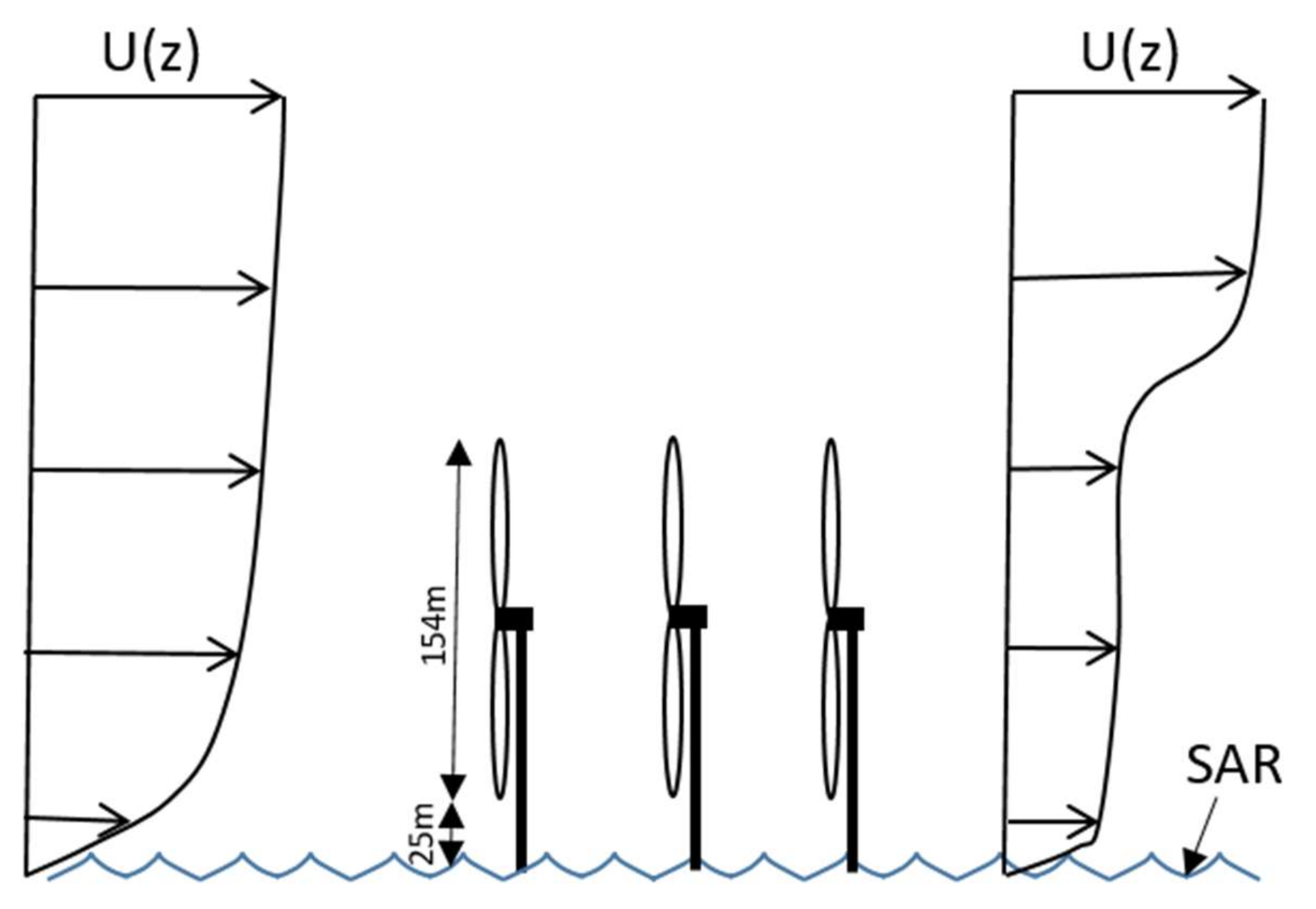
Comparisons of SAR wind fields against other data sources usually involve vertical extrapolation since the SAR winds and reference measurements are obtained at different levels above sea level. Logarithmic wind profiles are then assumed, which are not necessarily realistic in the wake of wind farms, where the atmosphere is not in local equilibrium. A semi-empirical model for wind profiles in the wind farm wake has been proposed [15], but validation is missing. Further, SAR observations may be influenced by oceanic currents and waves [21], whereas, reference data sets represent the atmospheric conditions only.
Ground based dual-Doppler radars can remotely sense line of sight wind speeds accurately over distances of tens of kilometers and new devices have recently been built for wind measurements [22,23]. This measurement technique can provide new insight about wind farm wakes in 3D with a high spatial and temporal resolution. During the BEACon measurement campaign, conducted by the wind farm developer Ørsted, two Doppler radars measured the horizontal wind speed over several heights covering the surroundings of the Westermost Rough wind farm in the United Kingdom and wind farm wakes were traced over several kilometers [24]. Co-located wind fields are available from the SAR sensors on board the Sentinel-1 A/B missions.
The objective of this paper is to characterize the spatial wind speed variability in the near and the far wake of large offshore wind farms based on spaceborne SAR and ground based dual-Doppler radar observations. For the first time, large scale wind measurements from SAR and Doppler radars will be compared. We will examine three selected cases and quantify velocity deficits from all the co-located SAR and Doppler radar observations. The paper is structured as follows: Section 2 gives an overview of the investigated location and data sets. In Section 3, we classify free stream and waked regions. Section 4 presents three case studies; one case with observations of near and far wake and two cases showing the near wake with undisturbed inflow conditions. Additionally, mean values derived from all the available cases are presented. In Section 5 and Section 6, we discuss and conclude on the presented findings.

2. Location and Data

2.1. Wind Farm

This analysis focuses on the wind farm Westermost Rough off the United Kingdom east coast. It is a medium sized offshore wind farm located between 8 and 14 km from the shore. The wind farm consists of 35 turbines placed in a regular grid with a nameplate capacity of 6 Megawatt. Their hub height is 102 m, while the rotor diameter D is 154 m. Figure 1a shows the layout of the wind farm with internal spacings of the turbines 950 m or 6.2D and 1140 m or 7.4D. There is a gap in the regular grid in rows C and D. Figure 1b shows the coastline to the southwest of Westermost Rough and the wind farm Humber Gateway 20 km to the south.
Figure 2 shows a sketch of the wind profile upstream of a wind farm (distance between turbines not to scale) and downstream in the turbine wake. The wind speed in the wake is reduced due to energy extraction of the wind turbines. SAR measurements are taken at the surface of the ocean, whereas the wind farm wake is generated in the rotor swept area from 25 m to 179 above the ocean surface.

2.2. Wind Speeds from SAR

Sentinel-1A/B SAR images are collected covering Westermost Rough and its surroundings. Images are in Interferometric Wide (IW) swath mode with vertical polarization and are downloaded in the medium Ground Range Detected format, which is delivered with a 40-m spatial resolution [25]. Sentinel-1 data is distributed by the European Union’s Copernicus program and can be used free of charge for both research and commercial purposes. The satellites are in a sun-synchronous orbit and images are acquired in the morning around 6 am and the afternoon around 5 pm local time.
Figure 3 shows a SAR image off the United Kingdom east coast covering the waters around Westermost Rough. Land has a higher backscatter and shows up brighter than the sea to the east of the indicated wind farms. Bright spots are visible on the water that are caused by increased radar reflection from ships and wind turbines. Four wind turbine clusters are visible as bright dots in clear rows. The wind direction is 235° and darker areas to the east indicate lower backscatter from the ocean that we attribute to the decreased wind speed in the wind farm wake [2,14,26].
Wind speed maps are retrieved from the Sentinel-1 A/B observations using the GMF called CMOD5.N [27]. The SAR scenes have a spatial resolution in the order of a few meters, but further averaging is necessary to reduce inherent speckle noise and effects from long-period ocean waves. The data is therefore reduced to quadratic pixels of 500 m. Ancillary inputs regarding the geometry of the satellite trajectory and a priori wind directions are necessary to determine the wind speed, see [5] for an overview. Wind direction inputs come from the Global Forecast System (GFS) model [28] and are interpolated to the resolution cells of the satellite observations. Input data from a global model is chosen to show that results from the SAR wind retrieval can be applied at different wind farms than the cases presented here.
Wind retrievals within the wind farm can be contaminated by reflections from the wind turbines as illustrated in Figure 3. Therefore, it is not recommended to use those values quantitatively, though the raw satellite image can still contain qualitative information of the flow patterns within the wind farm [26]. The wind speed maps retrieved from Sentinel-1 A/B are available from an archive at the Technical University of Denmark [29].

2.3. Wind Speeds from Dual-Doppler Radars

Pulsed radars can record returned radar waves that are Doppler shifted depending on the wind speed. The component of the wind velocity vector along the line of sight of the radar beam is measured with an accuracy of 0.03 m/s [22,23]. Two X-band Doppler radars have been deployed for the BEACon measurement campaign between 2016 and 2018, see Figure 1b. The radars have a beam width of 0.5°. A range resolution of 15 m independent of distance is reached by pulse compression. The radars scan between 0.2° and 1.4° elevation with 0.1° increments over an arc of 60° of azimuth covering Westermost Rough and the surrounding area with one full scan completed in 64 seconds. Quality control is performed on the data to exclude radar artefacts. The maximum range of the systems is 35 km and the areas covered by the radar scans are indicated in Figure 1b.
The scans from the two radars are combined into horizontal wind speeds and wind directions [23] on a UTM grid with 50 m horizontal and 25 m vertical resolution with heights between 50 m and 250 m. Reconstruction of the horizontal wind speed and wind direction requires independent line of sight wind speeds from two radars. This reconstruction works best when the beams cross each other perpendicularly and uncertainties increase as the angle between the beams decreases.

2.4. Ancillary Data

The wind farm SCADA system measures and records wind farm parameters. We use an aggregated yaw signal from all the turbines as indicator of the wind direction. This SCADA wind direction has been calibrated using turbine pairs near the wind farm perimeter. The offset in the SCADA wind direction is derived by comparing the profile of relative power as a function of wind direction with the expected wind direction of maximum power loss given the geometry of the layout [30]. The SCADA wind direction is used as a reference wind direction for classifying SAR images since it would be available at other wind farms as well.
CFSR2 (Climate Forecasting System Reanalysis) reanalysis data is used to determine differences in the sea and air temperature [31]. This temperature difference is used as a qualitative proxy for atmospheric stability estimates.

3. Methods

Classification of Upstream and Wake

Doppler radar measurements cover both the region upstream of the wind farm and the wake region downstream. Three distinct areas of the wind field are defined based on the SCADA wind direction (see Figure 4): 1) “upstream”, defined as the region upstream of the wind farm; 2) ”wake”, the area downstream of the wind farm; 3) “side”, as the areas adjacent to the wake. Wind retrievals within a buffer of 500 m surrounding the wind farm are discarded since SAR winds are not reliable here due to reflections from the wind turbines. This classification is used whenever averaged properties of the respective regions are calculated. This does not reflect a post-processing present throughout the analysis. The wind speed U and direction W D are spatially averaged over each of these areas. The area is denoted in a subscript (up, wake) and the measurement device in a superscript (SAR, DR).
The turbulence intensity (TI) is traditionally measured from a time series at a single location. For Doppler radar wind measurements this is not convenient as the temporal sampling frequency is low. One alternative is using TI derived from the instantaneous wind field itself. [32] suggested a method to derive fields of TI from dual-Doppler radar measurements. For the purpose of estimating the upstream TI, we find it sufficient to use the entire upstream area:
T I u p D R = U D R U D R 2 U D R
where U is the instantaneous wind speed and [*] denotes the spatial average, in this case for the region “up”.

4. Results

For the purpose of this study, we focus on wind fields from the dual-Doppler radars near the timestamps of the satellite overpasses. In order to study the wake in detail, we require that Doppler radar scans show at least part of the wind farm wake and the area upstream of the wind farm. A total of 18 Doppler radar scans fulfill this criterion and will form the basis of the further analysis. These are listed in Table 1. Wind speeds, wind directions and turbulence intensities in Table 1 are spatial averages over the areas defined in Figure 4.
Three cases from Table 1 are analyzed in more detail. The first case presents the evolution of a wind farm wakes from the near wake close to the far wake several kilometers downstream of the last turbines. The two following cases represent inflow conditions that are not disturbed by upstream land or wind farms.
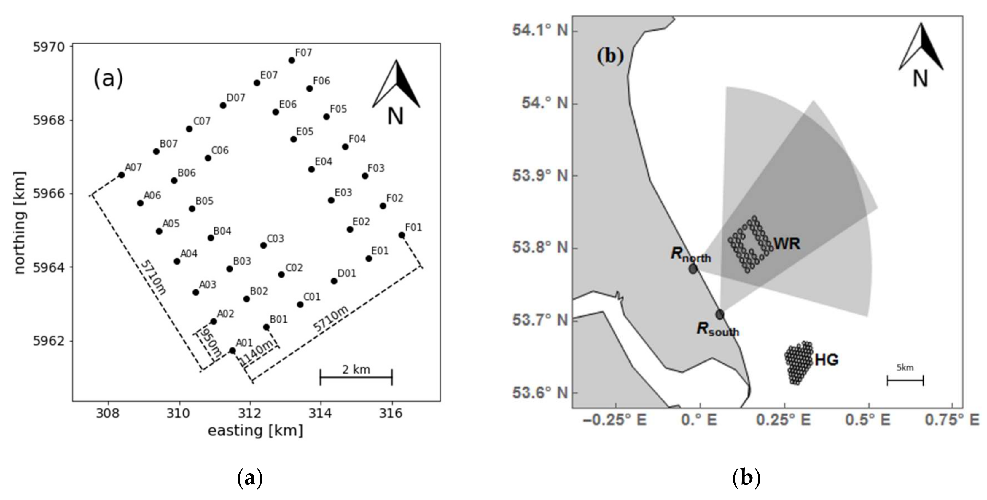
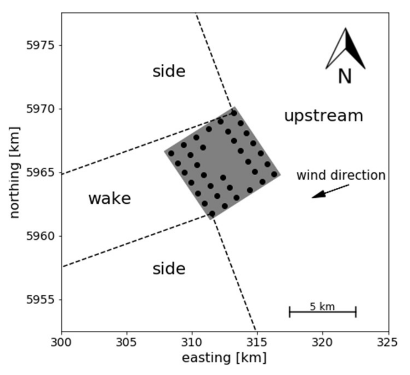
Due to the radar configuration and scanning strategy, the first case needs winds from southwest, see Figure 1. Wind speeds need to be in a range where wakes are expected, ideally between cut in where a wind turbine starts operating and rated wind speed where it reaches its rated power. We further require that the wind conditions are steady, in other words, no large temporal changes occur. The case from 04-10-2017 fulfils these requirements and will be presented as “Case 1”.
In Section 4.2, two additional cases are presented, where the inflow conditions are not disturbed by upstream land or wind farms. The aim is to compare two cases where the wind conditions are similar in regard to wind direction and speed, but wakes are depicted differently in SAR. The aim is to identify possible reasons for differences in the characterization of wind farm wakes from SAR. These conditions are fulfilled by cases 09-04-2018 and 27-04-2018 referred to as “Case 2” and “Case 3” respectively.

4.1. Case 1: Evolution of the Wake

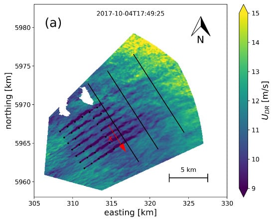
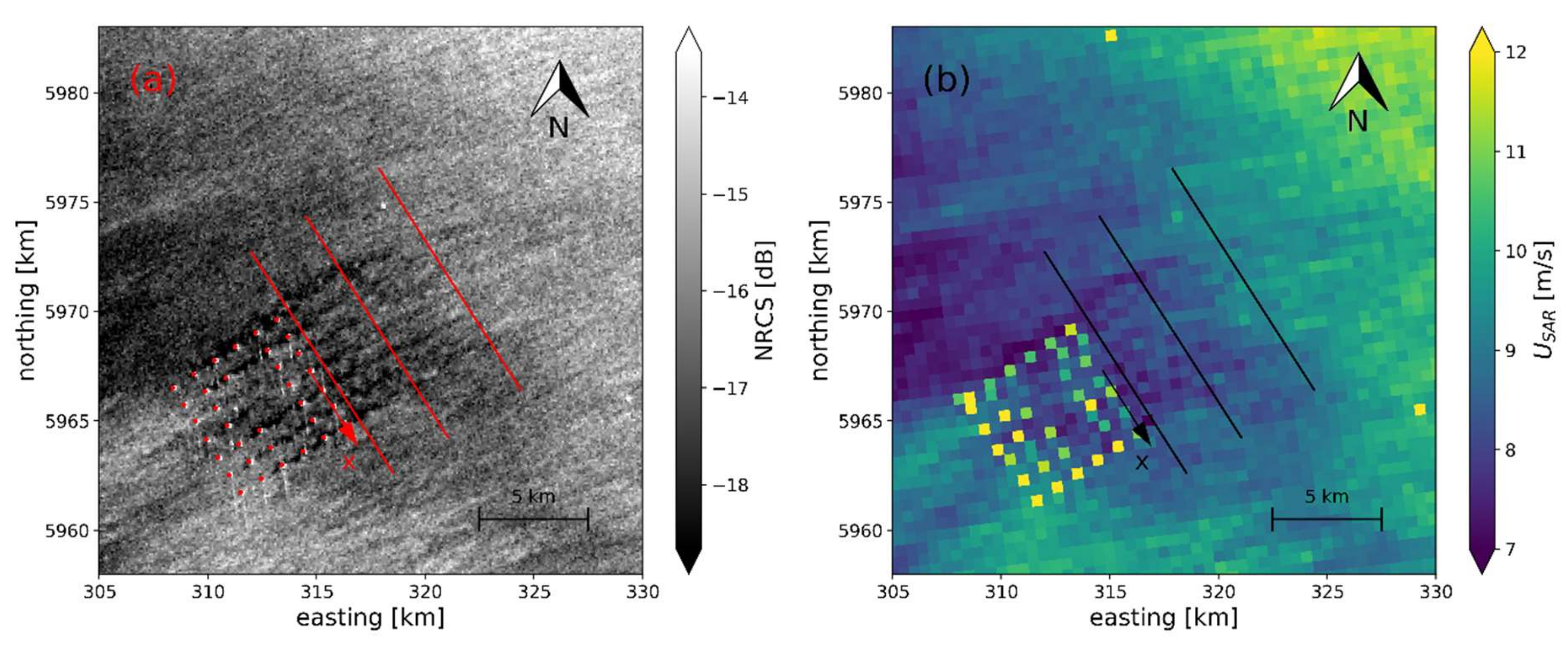
Figure 5 shows the NRCS and retrieved wind speed around Westermost Rough for Case 1 (04-10-2017 at 17:04) and 
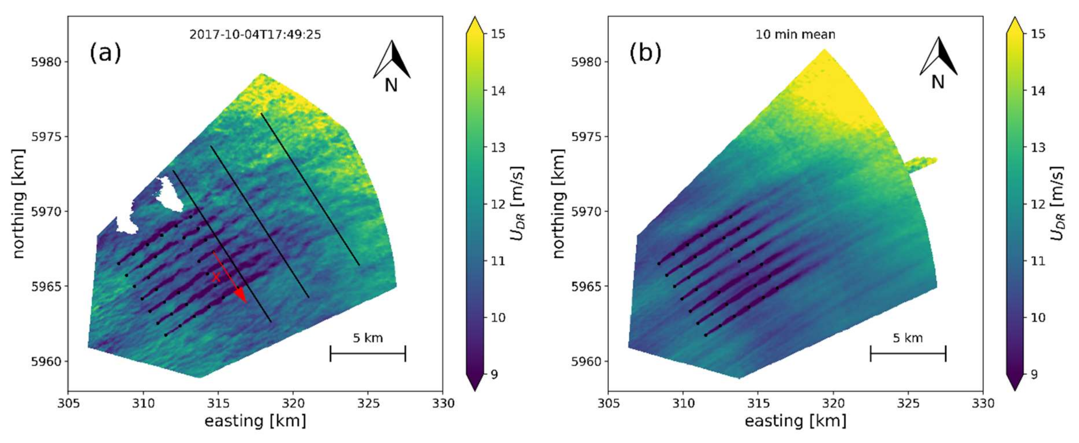
Figure 6 shows the dual-Doppler reconstructed wind field. The position x on the transect is defined as the cross-wind distance from the center turbine F04 as indicated by the arrow.
The intensity of the NRCS in Figure 5 varies over the image with strong backscatter where the turbines are located. Northeast of Westermost Rough dark streaks indicate an area of lower NRCS. The wind direction is 235° which locates these features downstream of the wind turbines. We associate this change in backscatter with the reduced wind speeds in the wake of the wind farm. Observing the structure more closely, we can determine that the streaks are in line with the wind turbine rows in the northeasterly direction. Streaks are present for approximately 7 km downstream of the wind farm. A reduction in the backscatter does not appear directly downstream of the first turbine in row A, but rather between row B and C, which is consistent with the wakes expanding beyond the rotor area and reaching the surface after a finite propagation distance in line with findings from [26].
Dual-Doppler radar reconstructed wind speeds are available on a grid covering the wind farm and a large area downstream. Figure 6 shows two such wind fields: Figure 6a shows an instantaneous snapshot of the wind speeds from the BEACon radars measured less than a minute from the SAR image acquisition, and Figure 6b shows the ten-minute mean wind speeds constructed from 9 individual scans around the same time. The instantaneous wind field shows more variations as expected from a turbulent wind field. Small scale variations are reduced in the averaging process in Figure 6b.
We can make several observations from the instantaneous wind field in Figure 6a. The wind speed around the wind farm is not uniform but has characteristic turbulent features. Wakes are present downstream of each wind turbine row and individual wind turbine wakes overlap with wakes from downstream turbines. The wakes are aligned with wind turbine rows, see Figure 1 (we will call them “row wakes” from here on) and extend downstream of the wind farm and stay separate for several kilometers before starting to merge. The row wakes downstream of the wind farm in the south are more pronounced than in the north.
In the mean wind field in Figure 6b, turbulent structures are reduced due to the averaging. Wakes in row 01 are exactly aligned while wakes in row 07 are slightly misaligned towards more northerly directions. For the rows in between, this effect seems to be gradually changing. The wind speed reduction in the centre of the wake is less pronounced than on the sides when the individual row wakes start to merge. This corresponds to a reduced number of turbines in row 04 and 05. The length of the wind farm wake is similar between the northern and southern side.
A qualitative comparison of the SAR image in Figure 5 and the Doppler radar measurements in Figure 6 reveals some similarities. Streaks of reduced backscatter and distinguishable wind farm wakes are structured as lines downstream of the wind farm with a similar extent and the wake downstream of the wind farm center seems to be less pronounced than at the edges. Some clear differences are also present. The SAR image appears noisier, which can be attributed to speckle. Wind turbine wakes in Doppler radar measurements appear directly downstream of turbines in the front row (A), while they appear further downstream in the SAR image. The most pronounced wake in the SAR image is located at the northern row while the Doppler radars indicates a more pronounced wake in the south.

Cross-Wind Transects

In order to go from a qualitative to a quantitative comparison, wind speeds are extracted from transects outlined on the SAR the Doppler radar wind maps. SAR observations at the resolution of Figure 5 are too noisy for accurate wind speed retrieval and further averaging is needed prior to wind retrieval processing. Averaging of SAR images to reduce speckle noise should be done over homogenous areas. As described in Section 2.2, the processing of the archived data used quadratic pixels of 500 m which will be denoted as “default” processing. Figure 5 and Figure 6 show that wakes are anisotropic in their length scale. The characteristic cross-wind scale is on the order of one rotor diameter, which is 150 m for this wind farm, while wakes extend several kilometers in the stream-wise direction. A second type of averaging is performed using rectangular boxes aligned with the wind direction. Pixels are averaged over boxes with 150 m in the cross-wind direction (corresponding to one rotor diameter) and 1000 m in the stream-wise direction, which will be denoted as “aligned” processing. This process is not actively searching for wake patterns but rather represents a different averaging process.
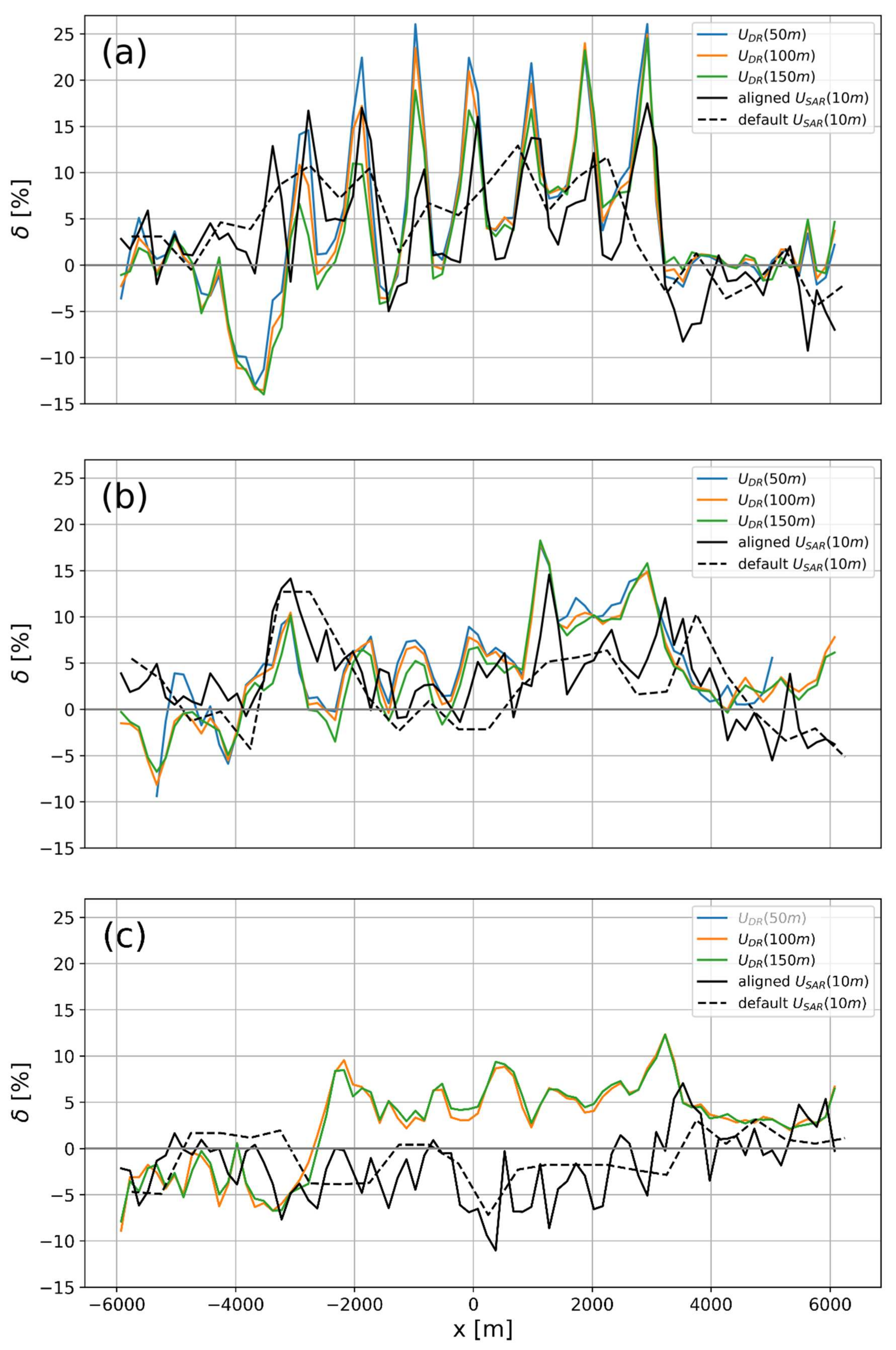
We choose three transects: Between 200 and 1200 m downstream (in stream-wise direction) of turbine row F that we denote as 700 m corresponding to the center of the transect. Similarly, transects at 3700 and 7700 m are defined. Transects and the coordinate system used are shown in Figure 6. Instantaneous Doppler radar wind speeds from Figure 6 are averaged over the same areas, as aligned processing to make the datasets comparable. Wind speeds are presented as velocity deficits compared to free stream wind speeds to the sides of the wind farm wake:
δ x =   U f r e e s t r e a m U w a k e x U f r e e s t r e a m
We define the free stream as the mean wind speed outside the wake at 4000 m < |x|. The reference wind speed is an average between both sides to account for spatial variations. Figure 7 shows wind speeds from SAR and Doppler radars on the three transects 700 m (a), 3700 m (b), and 7700 m (c) from the wind farm. The coordinate system is defined by the arrow in Figure 5 and Figure 6.
At 700 m downstream in Figure 7a, Doppler radar velocity deficits show seven distinct row wakes with velocity deficits between 6% and 26%. Velocity deficits tend to decrease with height, more so in the north (negative x). We can observe that SAR velocity deficits with aligned processing follow observations from the Doppler radars remarkably well. Local maxima occur at the same positions indicating that individual row wakes are at the same position in SAR and Doppler radar measurements. A general trend shows SAR velocity deficits to be lower with the exception being the wake at −3000m, where SAR velocity deficits are higher. SAR velocity deficits from default processing do show an overall velocity deficit in the wind farm wake but are unable to detect individual wakes. Between −4500 and −3000 m there is an area of negative velocity deficit, i.e., an area of higher wind speed, in the Doppler radar data that is not present in the SAR. This could likely be a gust that is present at measurement heights of the Dual-Doppler radar but not at the sea surface where SAR measurements are obtained.
Figure 7b shows transects at 3700 m downstream. A distinct velocity deficit measured from the Doppler radars is visible and row wakes from Figure 7a have started to merge. There are still distinct maxima at −3000, 1200, and 3000 m. Aligned SAR processing picks up these maxima but the locations can be slightly shifted, while default processing does not represent this structure well. At 7700 m in Figure 7c, Doppler measurements from 50 m are not available anymore due to the inclination of the radar beams. At 100 m and 150 m, there is still noticeable velocity deficit from the Doppler radar measurement, though smaller than for transects closer to the wind farm. Velocity deficits are highest at −2200 and 3000 m. These locations are linked to the row wakes on the side of the wind farm where most upstream turbines are located, as seen in Figure 1. Velocity deficits from SAR do not show a wake deficit anymore for neither processing method.

4.2. Case 2 and 3: Wakes at Similar Wind Conditions

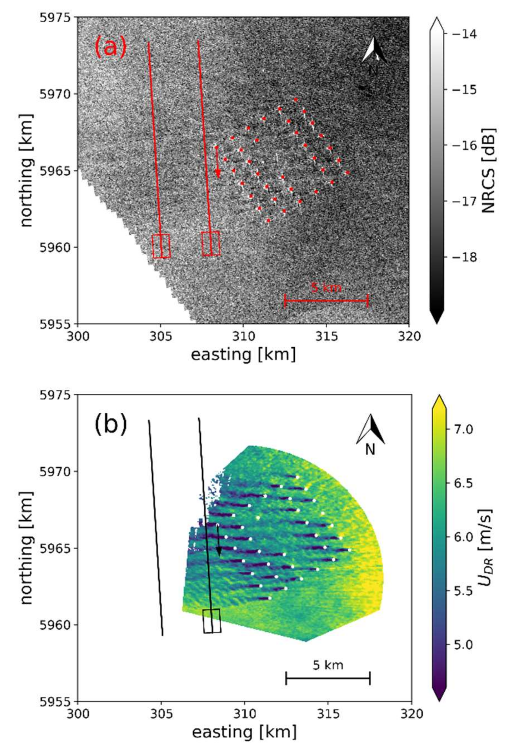
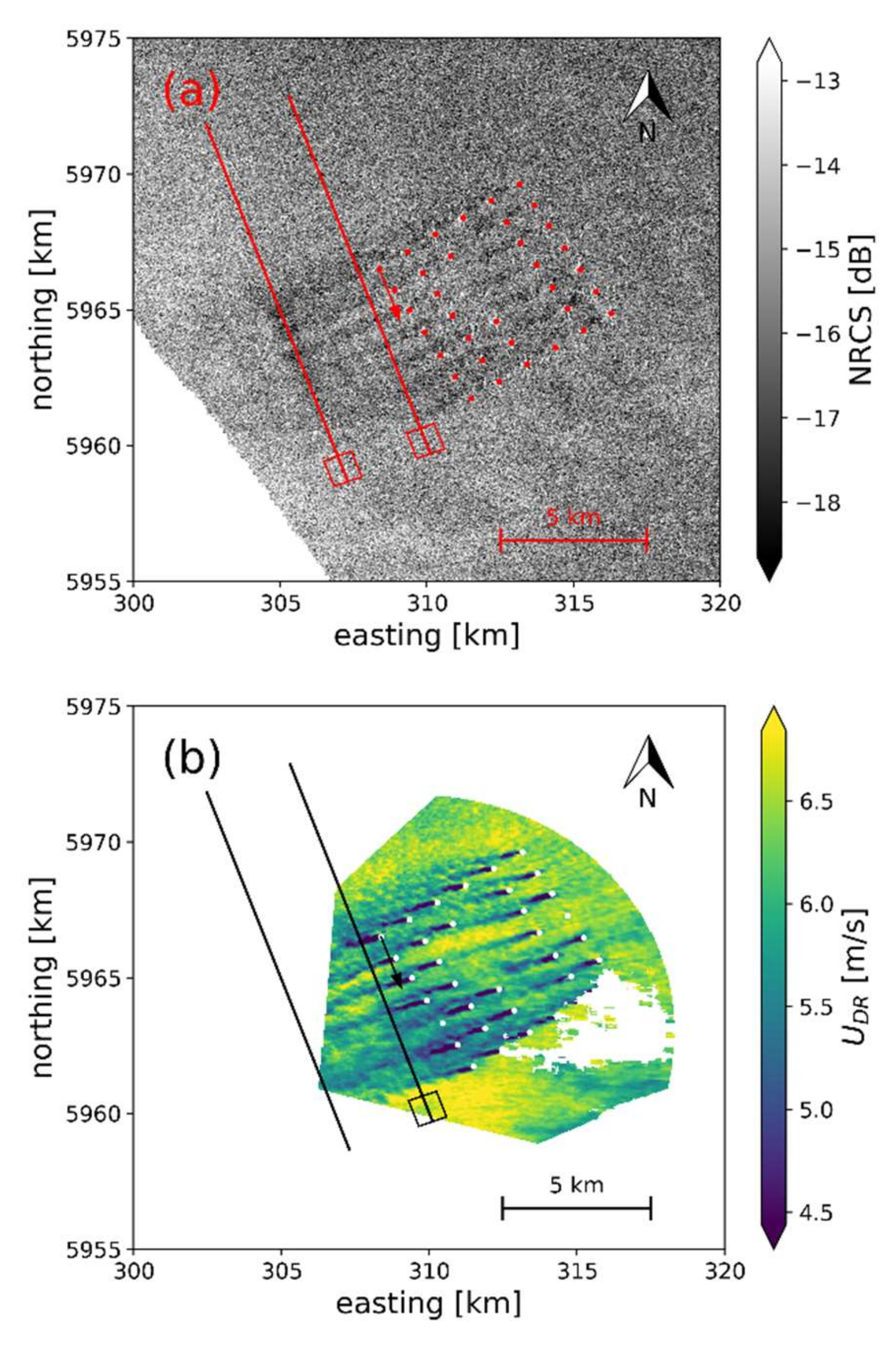
In the following, two examples are presented that are similar in terms of wind speed and direction. Case 2 occurs on 09-04-2018 where the wind direction obtained from the wind farm is 93°. Case 3 occurs 18 days later on 27-04-2018 where the wind direction is 73°. SAR backscatter from the ocean surface and Doppler radar winds at 100 m are presented for Case 2 in Figure 8 and for Case 3 in Figure 9.
The SAR image of Case 2 in Figure 8a does show an area of slightly lower NRCS downstream of the wind turbines, while the Doppler radar at 100 m is showing clearly visible wakes. The directions of the wakes are approximately diagonal to the grid-like structure of the wind farm rows. Wakes stay separated in the wind farm until they leave the Dual-Doppler domain to the east. The SAR image from Case 3 in Figure 9 very clearly shows dark streaks downstream of the wind farm. The Doppler radar measurement shows the presence of wind farm wakes in a similar area. Wakes start merging fast downstream of the southern part of the wind farm.

4.2.1. Cross-Wind Transects

Transects are defined at a distance of 700 m and 3700 m downstream of turbine A07 and 7 km to either side in cross-wind direction as shown in Figure 8 and Figure 9. Wind speeds on the transects are calculated as in Section 4.1. Dual-Doppler data coverage not influenced by wakes is limited to the north and the free stream is defined as the small section at the southern end of the transect indicated as a box in Figure 8 and Figure 9. Transects of the resulting velocity deficits are shown in
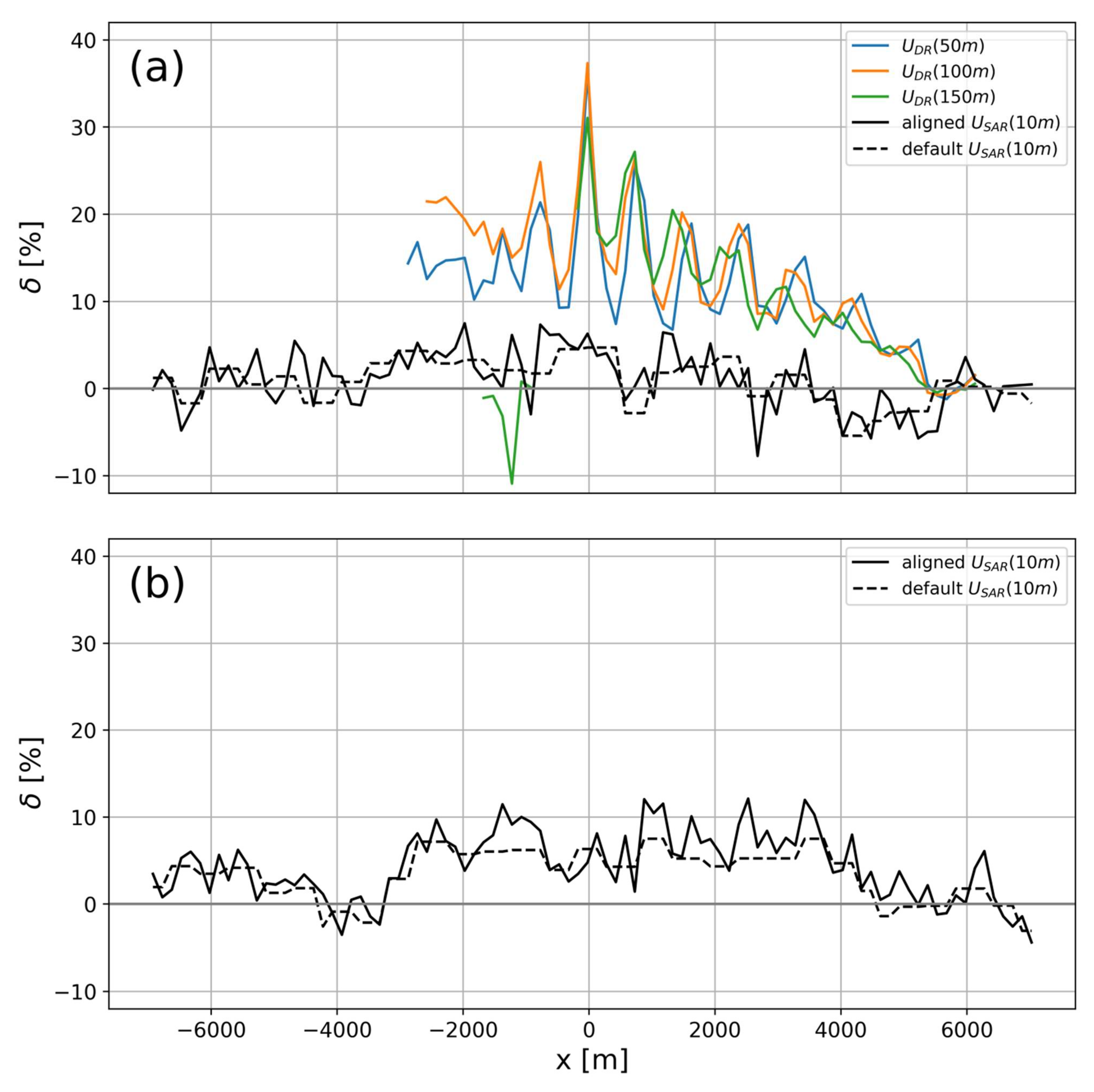
 Figure 10 and Figure 11.
For Case 2 in Figure 10a, the Doppler radar measurements clearly show individual wakes and an overall reduction of the wind speed with a maximum velocity deficit around 35%. The velocity deficit is highest at 0 m cross-wind distance which is closest to the wind farm. Velocity deficits from SAR range between −6% and 8% but do not follow the individual wakes as seen from the Doppler radars. There is a tendency towards positive velocity deficits from −3000 m to 2000 m where the wind farm wake would be expected and little difference between wind speeds retrieved with default or aligned processing. The second transect 3700 m downstream of the wind farm in Figure 10b shows a more clearly pronounced wake with positive velocity deficits between 2% and 12% between −3000 m and 4000 m cross-wind where the wake is expected. No Dual-Doppler measurements are available here due to the experimental setup.
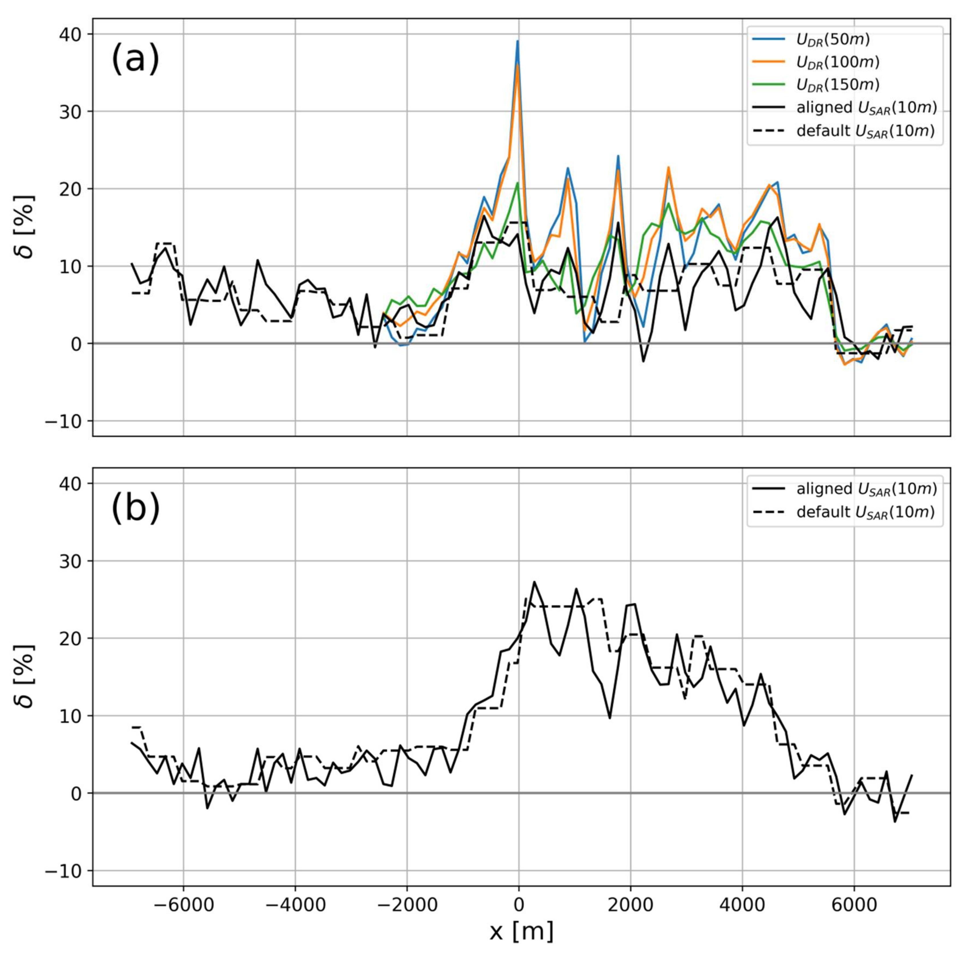
Doppler radar velocity deficits for Case 3 at 700 m downwind distance in Figure 11a clearly show the velocity deficit downstream of tubine A07 (at 0 m cross-wind) and also clearly distinguishable wakes at 900 m and 1800 m in the cross-wind direction. From 2500 m to 5500 m wakes are overlapping and individual turbine or row wakes are not distinguishable. Similar to Case 1, aligned SAR processing follows the structure of the individual wakes well, while default SAR processing does not show individual wakes but the overall velocity reduction. In general, SAR shows less velocity deficit than measured from the Doppler radars. SAR velocity deficits at 3700 m downstrem in Figure 11b show a clearly pronounced wake with velocity deficit up to 27%. The aligned processing shows peaks in the velocity defict indicating that the wakes are not fully merged yet. The position of the peaks is consistent with the turbine spacing indicating that individual turbine wakes are causing these peaks. The overall velocity deficit measured by SAR at 3700 m downstream is larger than at 700 m.
The two cases were chosen, since the wind speed at 100 m and the wind direction are very similar. From comparisons of the wind fields alone, it is not clear why wakes in the SAR image clearly follow Doppler radar measurements in Case 3 but not in Case 2.

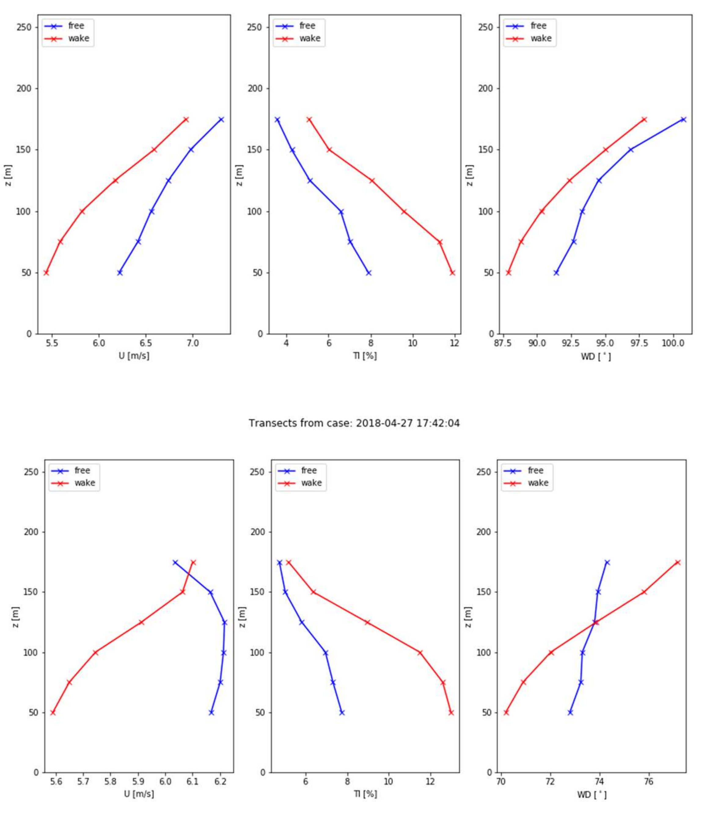
4.2.2. Wind Profiles

In the following, the vertical structure of the atmosphere is examined. Doppler radar measurements are available at heights between 50 and 250 m but we limit the height to 175 m due to low measurement availability above. Profiles are calculated from spatial averaging of instantaneous wind speeds in the free stream region, see Figure 4. The availability of the Doppler radar measurements is not constant over the height. In order to avoid artefacts from averaging different horizontal positions we require that measurements are available for all heights at the considered locations. Profiles of the mean wind speed, wind direction, and turbulence intensity are calculated.
Figure 12 shows the resulting profiles. Upstream wind profiles for Case 2 shows an increase in the wind speed with height. The wind speed upstream for Case 3 shows little change between 50 and 125 and a wind speed reduction above. The averaged wind profiles in the wake are similar between the cases. The change in wind direction with height (wind veer) upstream is stronger for Case 2 with changes from 91° to 100° but weaker for Case 3 ranging from 73° to 74°. Profiles of turbulence intensity are similar between the cases with higher TI closer to the ground and a general increase in the wind farm wake.

4.2.3. Atmospheric Stability

Wind farm wakes are known to be stability dependent [3,33] and differences in the atmospheric stratification could be an explanation of how SAR captures wind farm wakes [14,15]. Atmospheric stratification or stability can be described as the degree of mixing in the atmosphere; unstable conditions have a high degree of mixing while stable conditions are characterized by a low degree of mixing. Stability can best be estimated from atmospheric flux measurements or measurements of temperature differences but no such measurements are available at Westermost Rough. Instead the atmospheric stability is estimated from the measurements and models available to us. We will use the following parameters: 1) the shear exponent α in Equation (3), 2) the wind direction changes with height (veer), and 3) temperature differences between air and sea from CFSR model. Individually, determining stability from these sources can be misleading but together they can provide a good indication for atmospheric stratification. Results are summarized in Table 2 including an average of the velocity deficit from Figure 10 and Figure 11.
(1) Shear Exponent
A typical engineering model for wind profiles is the power law:
U z =   U r e f z z r e f α
where z r e f and U r e f are the reference height and the associated wind speed and α the shear exponent. A shear exponent lower than 1/7 is associated with unstable stratification and a shear exponent higher than 1/7 with stable stratification [34]. Fitting the wind profiles shows that Case 2 has a shear coefficient of 0.07 and Case 3 has a shear coefficient of −0.02 indicating that both cases occur at unstable stratification.
(2) Wind Veer
The wind veer is expressed as the change in the wind direction between 50 and 175 m. High (low) veer is associated with stable (unstable) atmosphere [35]. A wind veer of 1° for Case 3 and 9° for Case 2 is observed. Wind veer at an onshore site was quantified by [36]. For similar wind speeds they found wind veers in the order of 5° for unstable, 8° for neutral, and 20° for stable atmospheric. We take this as an indication that Case 3 is likely unstable while Case 2 lies between neutral and stable condition.
(3) Air-Sea Temperature Difference
Reanalysis data can provide modelled sea surface temperatures (SST) and air temperatures. The difference in temperatures gives an indication of stability. Case 2 has air that is slightly warmer than the sea indicating stable conditions but the temperature difference is small. Case 3 has cold air over warm water indicating unstable stratification.
From values presented in Table 2 we see that a combination of a low wind veer, low shear exponent, and a negative air-sea temperature difference points to unstable stratification for Case 3. For Case 2 the picture is less clear. The wind veer points to neutral to weakly stable stratification, the temperature difference from CFSR points to slightly stable stratification while the shear exponent suggests unstable stratification. The mean wind profile in Equation (3) is only valid within the surface layer, which can be as low as a few tens of meters for a stable marine boundary layer. It is likely that measurements between 50 and 175 m are at least partially outside this layer if the atmospheric stratification is stable. From this we deduct that Case 2 likely occurs under weakly stable conditions though some uncertainty remains. A detailed discussion on the occurrence of wakes for Case 2 and Case 3 is given in Section 5.

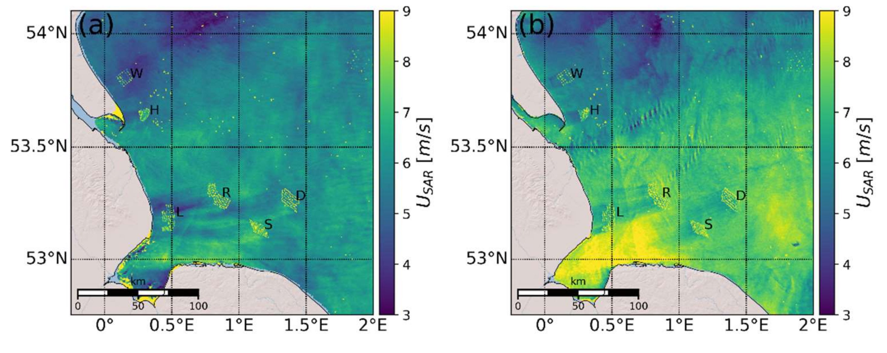
4.2.4. Wakes of Surrounding Wind Farms

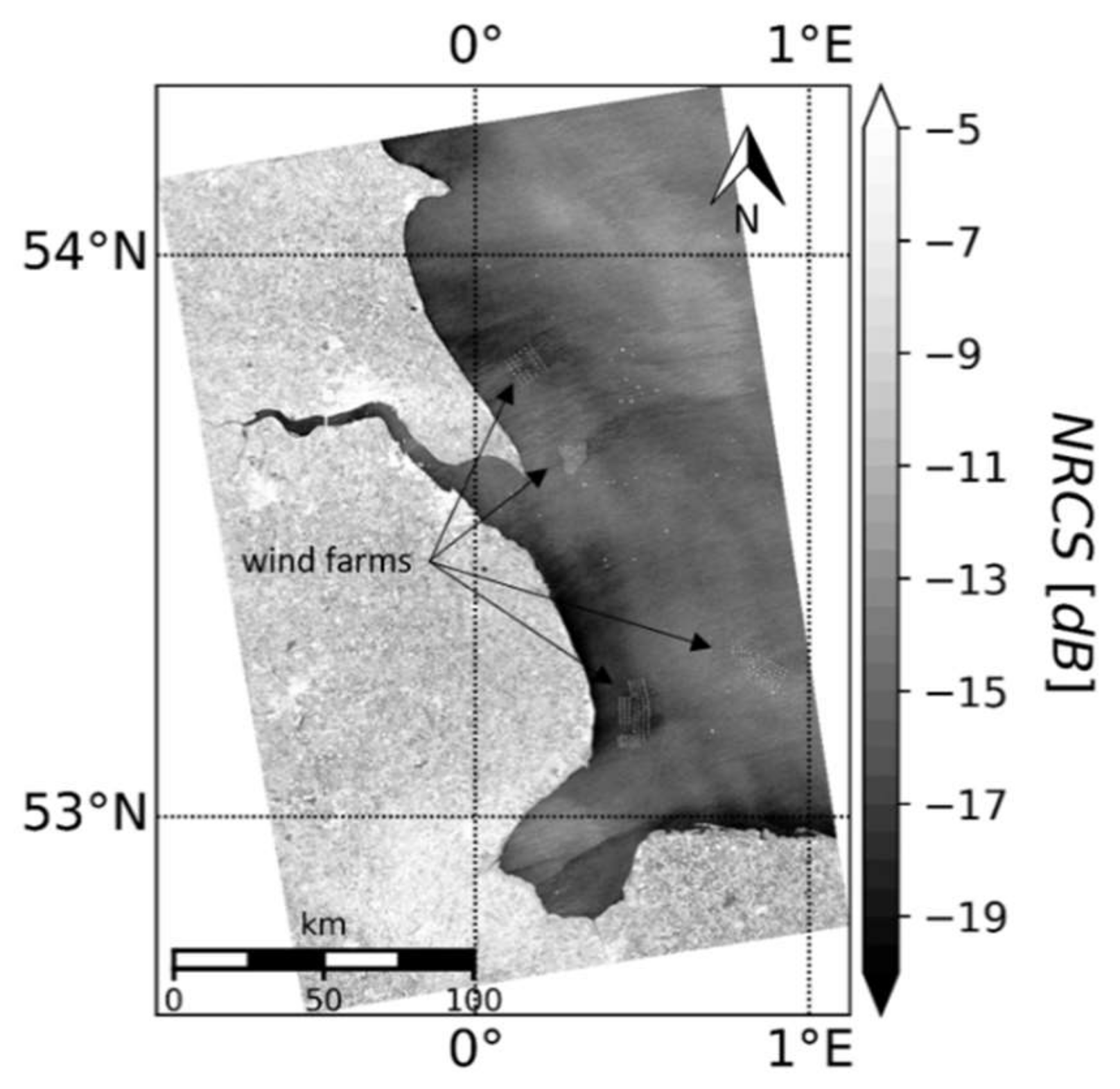
SAR wind fields from Case 2 and Case 3 in Figure 13 cover five additional wind farms, which are located in the vicinity of Westermost Rough. The positions of the wind farms are marked in the images and are visible due to reflection of the turbines. Some ships influence the retrieval and are visible as scattered points. SAR winds for Case 2 are shown in Figure 13a. Wind farm wakes are visible downstream of Race Bank, Sherinham Shoal, Dudgeon, and Humber Gateway. Wakes extend for several tens of kilometres. For Case 3 in Figure 13b winds increase to the south. Wind farm wakes are visible downstream of all wind farms. For Dudgeon and Sherinham Shoal the velocity deficit disappears after approx. 10 km while the wake of Race Bank extends until it reaches Lincs.

4.3. Overview of All Wake Cases

The presented cases in Section 4.1 and Section 4.2 had very good coverage from the Doppler radars and showed that wakes from SAR and Doppler radar can be comparable. The entire data set is utilized to determine how SAR and Doppler radars measure velocity deficits on average. For this purpose, the velocity deficit is calculated from SAR and Doppler radar measurements for the same horizontal positions. SAR winds are retrieved using 500 m resolution of the default processing. The Doppler radar measurements are averaged on the same 500 m grid to collocate the measurements.
We assume that variations in the wind speed from unsteadiness and inhomogenuities are the same in SAR and Doppler radar velocity deficits. The difference between the velocity deficits should then properly reflect how much deviation SAR velocity deficits have in the near wake compared to the more direct wind speed measurement from the Dual-Doppler radars. The assumptions are tested by calculating velocity deficits between the areas upstream and to the side of the wind farm, see Figure 4. The velocity deficit to the side should then be identical as measured from SAR and Doppler radars. A detailed explanation for this argument can be found in the Appendix.
We analyse SAR and Doppler radar wind fields and calculate velocity deficits for the wake. We require available data at Doppler radars at all heights between 50 and 175 m, at least ten 500 m resolution cells in the upstream and wake region, and no more than 60 s difference between the SAR image and the Doppler radar scan. A total of 12 scenes from Table 1 fulfil these requirements and averaged results of the velocity deficits are presented in
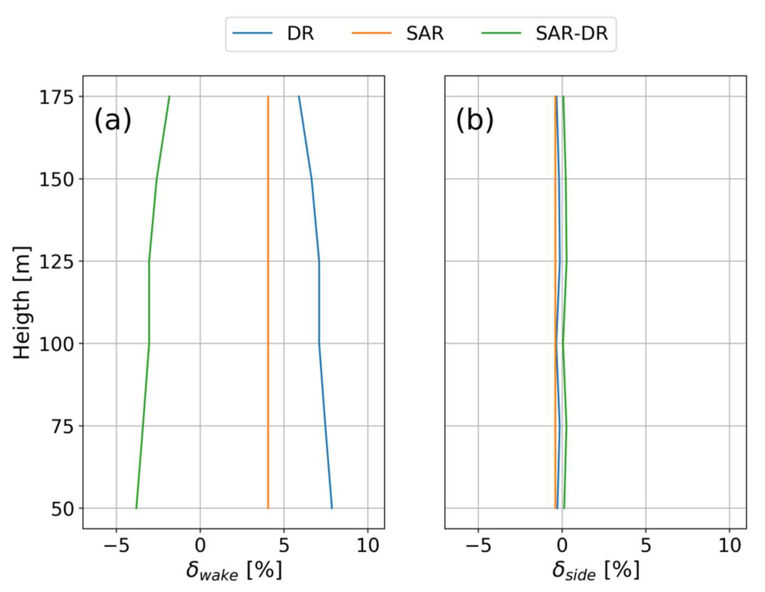
 Figure 14.
The velocity deficit in the wake from SAR and Doppler radar together with their difference are plotted in Figure 14a. Results for SAR are plotted over all heights to make comparisons easier even though results are associated with 10 m height. The velocity deficit from SAR is 4% while Doppler radar velocity deficits range from 6% to 7.5% depending on the height. Velocity deficits between the upstream region and the sides are plotted in Figure 14b. Velocity deficits are small here and differences between SAR and Doppler radar are minor. This is taken as an indication that the assumption of SAR and Dual-Doppler radar measuring variations in the wind speed similarly is fulfilled.

5. Discussion

The presented analysis shows the first wind farm wakes estimated from SAR with coinciding 3D atmospheric measurement from Doppler radars of the near and far wake. In the following, we will discuss differences in the structure of the wake as measured from SAR and Doppler radar with regards to atmospheric conditions.

5.1. SAR and Dual-Doppler Radar Wakes

Three cases with Sentinel-1 SAR scenes of wind farm wakes have been presented and wakes were present in all three SAR images. Wind fields measured from the Doppler radar at the same time confirmed the position of the wakes. Doppler radar measurements presented here can confirm that the low backscatter region typically observed downstream of wind farms [14] coincides with the wind farm wake.
The wake structure in the cross-wind direction is determined by local maxima and minima of the velocity deficit caused by individual turbines and turbine rows. To examine the wake structure, transects were defined at a distance of 700 m from the wind farm crossing the wind farm wake. For Case 1 and 3, coinciding velocity deficits from Doppler radars are located at similar positions. This finding raises confidence that the structure in the wind farm wake found in SAR images are really related to the wake in the atmosphere [26]. For Case 1 Doppler radar measurements are available for approx. 10 km downstream of the wind farm. The wake structure of SAR transects agrees better with Doppler radar measurements close to the wind farm than further downstream. The estimated velocity deficit is generally lower for the SAR than for the Doppler radar observations.

5.2. Quantifying Wake Differences

Lower velocity deficits from SAR compared to other reference data has been observed before from comparisons to data from Weather Research and Forecasting (WRF) model [2] and SCADA derived wind speeds [20]. Our attempt to quantify averaged differences in the velocity deficit from the presented data shows that SAR is underestimating by roughly four percentage points.
We hypothesize that differences in the VD measured from SAR compared to atmospheric wakes near hub height have two connected contributors: 1) Wakes are generated over the area of the rotor, here between 25 and 179 m and are typically strongest at hub height [37], while SAR measurements are taken at the ocean surface, where the velocity deficit can be expected to be smaller. 2) Reduced momentum in the wake needs to be transported to the ocean surface in order to leave an imprint in the SAR image. The magnitude of this transport is determined by the atmospheric stratification.

5.3. Wakes and Stability

Two cases with inflow conditions from the open ocean are presented that are similar in terms of the wind speed and direction. For Case 2 the wake in SAR images is much less pronounced compared with Doppler radar measurements while both SAR and Doppler radar show very similar wake behaviours in Case 3. Wind profiles and air-sea temperature differences indicate that atmospheric stratification is weakly stable for Case 2 and unstable for Case 3.
Large turbulent structures created from buoyancy are present under unstable conditions that cause a well-mixed atmospheric boundary layer. Reduced momentum in the wake is transported from hub height to the ocean surface and can be detected in the SAR images. The structure of the wake in the SAR images is very similar to the atmospheric wake measured from the Doppler radar. By contrast, under stable conditions buoyancy is attenuating large turbulent structures and low mixing reduces the momentum transport to the ocean surface. These observations are consistent with findings of [15] that the maximum of the velocity deficit in a SAR wind field occurs directly downstream of the wind farm for unstable conditions while being displaced further downstream for stable conditions. Our results indicate that SAR images can well detect the structure of the wake close to the wind farm under unstable conditions.
Case 1 has a temperature difference in CFSR of −0.3 K and wind speeds of 10.9 m/s indicating slightly unstable to neutral stratification. The wind profile cannot be used to infer the stratification due to disturbances from the upstream land. In the near wake the SAR derived velocity deficit follows the Doppler radar reference measurements well. A similar case with neutral stratification and where wind turbine rows are aligned with the wind direction is available in [26]. These results indicate that velocity deficits from SAR would also accurately describe the wake structure under neutral conditions but a more comprehensive analysis using accurate stability measurements is necessary to determine the threshold stability for this.

5.4. Sentinel-1 for Wake Studies

This study indicates that the wake structure of offshore wind farms can be detected from Sentinel-1 A/B images in IW mode as an alternative to observations from TerraSAR-X, which offers a higher spatial resolution [26]. Compared to TerraSAR-X, Sentinel-1 are openly available to industry and the research community alike, which makes application at any new location easier. The structure of the wind farm wake is well represented for unstable stratification when SAR winds are retrieved with aligned processing while it disappears in the default processing. For studies determining the wake structure we recommend using aligned processing to retain information on the wake structure and retrieve the typical velocity deficit maxima in the near wake.

6. Conclusions

Medium-resolution Sentinel-1 A/B SAR images can be used to observe the fine structure within wind farm wakes downstream of large offshore wind farms. For the first time, atmospheric measurements from Doppler radars covering the full wind farm wake region are available to confirm the position and structure of wakes as seen in the SAR imagery. Our study indicates that the detection of wakes in SAR imagery is dependent on the atmospheric stability. For unstable conditions, where strong temperature-driven vertical motions of the air column are present, the structure of wind turbine wakes is similar in SAR and Doppler radar reference observations. For stable conditions, where the air column above the sea surface is stratified with little momentum exchange between the different layers, the agreement between SAR and Doppler radar winds is poorer. On average, the velocity deficit estimated from SAR and Doppler radar observations downstream of the Westermost Rough wind farm in the UK is 4% and 8%, respectively. Considering that SAR data is available for end users free of charge whereas Doppler radar campaigns are rather costly, there is a potential for using SAR wind fields as large-scale reference data showing the spatial extent of wind farm wakes. The global wind energy industry could benefit from this type of information. We have presented a first comparison of co-located SAR and Doppler wind retrievals. Further analyses over other offshore wind farms around the world and with a higher number of co-located samples would strengthen the benchmarking of satellite-derived wake characteristics and improve our understanding of wind farm wake effects further.

Author Contributions

The authors contributions are as follows: conceptualization, T.A., M.B., N.G.N., and A.N.; methodology, T.A.; software, T.A.; validation, T.A., N.G.N., and A.N.; formal analysis, T.A., N.G.N., and A.N.; investigation, T.A., M.B., N.G.N., and A.N.; resources, T.A., M.B., N.G.N., and A.N.; data curation, T.A., M.B., N.G.N., and A.N.; writing—original draft preparation, T.A.; writing—review and editing, T.A., M.B., N.G.N., and A.N.; visualization, T.A.; supervision, M.B.; project administration, T.A., M.B., and N.G.N.; funding acquisition, M.B., and N.G.N. All authors have read and agreed to the published version of the manuscript.

Funding

This work received funding from the EU H2020 program under grant agreement no. 730030 (CEASELESS project).

Acknowledgments

We would like to acknowledge Ørsted for granting access to data from the Westermost Rough wind farm and their BEACon Doppler radar data, Johns Hopkins University Applied Physics Laboratory and the National Atmospheric and Oceanographic Administration (NOAA) for the use of the SAROPS system and the ESA for providing public access to data from Sentinel-1.

Conflicts of Interest

Nicolai Gayle Nygaard and Alexander Newcombe are employed at Ørsted AS, the provider of the dual-Doppler data set and the developer of the Westermost Rough wind farm. Merete Badger and Tobias Ahsbahs declare no conflicting interests.

Appendix

The velocity difference in the wake ( U i d e a l ) is the difference between the wind speed in the wake and a reference wind speed. Ideally, one would observe the same realization of the flow once with the wind farm ( U w a k e ) and once without the wind farm ( U r e f ).
U i d e a l =   U r e f U w a k e
Measuring this is not possible for field measurements because the wind farm either exists or does not exist. For a steady and homogenous flow the upstream wind speed ( U u p ) is equivalent to U r e f but in general the flow will be unsteady and inhomogeneous. If we assume that influences from inhomogeneity U i n h o m and unsteadiness U u n s t can be superimposed, we can write:
U r e f = U u p + U i n h o m + U u n s t
and for the velocity difference:
U i d e a l =   U u p U w a k e + U i n h o m + U u n s t
Capital letters denote spatial averaging over the areas “up” and “wake” in Figure 4. Our aim is to isolate the difference in velocity differences as measured from SAR and Doppler radars (DR). Assuming mean inhomogenuities ( Δ U i n h o m ) and local fluctuations ( Δ U u n s t ) to be the same between SAR and dual-Doppler radar measurements, the difference in the velocity difference U w a k e , d i f f becomes:
U w a k e , d i f f = Δ U i d e a l , S A R Δ U i d e a l , D R   U u p , S A R U w a k e , S A R U u p , D R U w a k e , D R =   Δ U w a k e , S A R Δ U w a k e , D R
For consistency with results from Section 4.1 and 4.2 we define these in terms of velocity deficit by assuming that the upstream wind speed is approximately the free stream wind speed.
δ w a k e   Δ U w a k e U u p
The right hand side of this equation can be measured. The assumption of Δ U i n h o m and Δ U u n s t to be the same between SAR and dual-Doppler radar can be tested using the area “side” in Figure 4. Defining the velocity difference between up and side:
U s i d e = U u p U s i d e =   U i n h o m U u n s t
Since there is no wake here, differences between the areas difference originate from inhomogeneity and unsteadiness. The differences of Equation (8) from SAR and dual-Doppler radar should be zero:
U s i d e , d i f f = U s i d e , S A R U s i d e , D R 0
Again for consistency this can be defined in terms of VD:
δ s i d e   Δ U s i d e U u p

References

  1. Wind Europe Offshore Wind in Europe: Key trends and statistics 2018. Available online: https://windeurope.org/about-wind/statistics/offshore/european-offshore-wind-industry-key-trends-statistics-2018/ (accessed on 15 November 2018).
  2. Hasager, C.B.; Vincent, P.; Badger, J.; Badger, M.; Di Bella, A.; Peña, A.; Husson, R.; Volker, P.J.H. Using satellite sar to characterize the wind flow around offshore wind farms. Energies 2015, 8, 5413–5439. [Google Scholar] [CrossRef] [Green Version]
  3. Platis, A.; Siedersleben, S.K.; Bange, J.; Lampert, A.; Bärfuss, K.; Hankers, R.; Cañadillas, B.; Foreman, R.; Schulz-Stellenfleth, J.; Djath, B.; et al. First in situ evidence of wakes in the far field behind offshore wind farms. Sci. Rep. 2018, 8, 2163. [Google Scholar] [CrossRef] [PubMed]
  4. Valenzuela, G.R. Theories for the interaction of electromagnetic and oceanic waves? A review. Boundary-Layer Meteorol. 1978, 13, 61–85. [Google Scholar] [CrossRef]
  5. Dagestad, K.-F.; Horstmann, J.; Mouche, A.; Perrie, W.; Shen, H. Wind retrieval from synthetic aperture radar, an overview. In Proceedings of the Seasar 2012 Oceanography Workshop, Tromso, Norway, 18–22 June 2012. [Google Scholar]
  6. Stoffelen, A.; Anderson, D. Scatterometer data interpretation: Estimation and validation of the transfer function CMOD4. J. Geophys. Res. Space Phys. 1997, 102, 5767–5780. [Google Scholar] [CrossRef]
  7. Hersbach, H.; Stoffelen, A.; De Haan, S. An improved C-band geophysical model function CMOD5. J. Geophys. Res. 2007, 112, 863–870. [Google Scholar] [CrossRef]
  8. Monaldo, F.; Thompson, D.; Beal, R.; Pichel, W.G.; Clemente-Colón, P. Comparison of SAR-derived wind speed with model predictions and ocean buoy measurements. IEEE Trans. Geosci. Remote Sens. 2001, 39, 2587–2600. [Google Scholar] [CrossRef]
  9. La, T.V.; Khenchaf, A.; Comblet, F.; Nahum, C. Exploitation of c-band Sentinel-1 images for high-resolution wind field retrieval in coastal zones (Iroise Coast, France). IEEE J. Sel. Top. Appl. Earth Obs. Remote Sens. 2017, 10, 5458–5471. [Google Scholar] [CrossRef]
  10. Lu, Y.; Zhang, B.; Member, S.; Perrie, W.; Aur, A.; Li, X.; Member, S.; Wang, H. A c-band geophysical model function for determining coastal wind speed using Synthetic Aperture Radar. IEEE J. Sel. Top. Appl. Earth. Obs. Remote Sens. 2018, 11, 2417–2428. [Google Scholar] [CrossRef] [Green Version]
  11. Monaldo, F.M.; Jackson, C.; Li, X.; Member, S.; Pichel, W.G. Preliminary evaluation of Sentinel-1A wind speed retrievals. IEEE J. Sel. Top. Appl. Earth. Obs. Remote Sens. 2015, 8, 2638–2642. [Google Scholar] [CrossRef]
  12. Hasager, C.B.; Badger, M.; Peña, A.; Larsén, X.G.; Bingöl, F. SAR-based wind resource statistics in the Baltic Sea. Remote Sens. 2011, 3, 117–144. [Google Scholar] [CrossRef] [Green Version]
  13. Ahsbahs, T.; Badger, M.; Karagali, I.; Larsén, X.G. Validation of Sentinel-1A SAR coastal wind speeds against scanning LiDAR. Remote Sens. 2017, 9, 552. [Google Scholar] [CrossRef] [Green Version]
  14. Christiansen, M.B.; Hasager, C.B. Wake effects of large offshore wind farms identified from satellite SAR. Remote Sens. Environ. 2005, 98, 251–268. [Google Scholar] [CrossRef]
  15. Djath, B.; Schulz-Stellenfleth, J.; Cañadillas, B. Impact of atmospheric stability on X-band and C-band synthetic aperture radar imagery of offshore windpark wakes. J. Renew. Sustain. Energy 2018, 10, 043301. [Google Scholar] [CrossRef] [Green Version]
  16. Nygaard, N.G.; Hansen, S.D. Wake effects between two neighbouring wind farms. J. Physics: Conf. Ser. 2016, 753, 32020. [Google Scholar] [CrossRef] [Green Version]
  17. Fitch, A.C.; Olson, J.B.; Lundquist, J.K.; Dudhia, J.; Gupta, A.K.; Michalakes, J.; Barstad, I. Local and mesoscale impacts of wind farms as parameterized in a mesoscale NWP model. Mon. Weather. Rev. 2012, 140, 3017–3038. [Google Scholar] [CrossRef]
  18. Schneemann, J.; Rott, A.; Dörenkämper, M.; Steinfeld, G.; Kühn, M. Cluster wakes impact on a far distant offshore wind farm’s power. Wind Energy Sci. 2020, 5, 29–49. [Google Scholar] [CrossRef] [Green Version]
  19. Jacobsen, S.; Lehner, S.; Hieronimus, J.; Schneemann, J.; Kühn, M. Joint offshore wind field monitoring with spaceborne sar and platform-based doppler lidar measurements. ISPRS Int. Arch. Photogramm. Remote. Sens. Spat. Inf. Sci. 2015, 7, 959–966. [Google Scholar] [CrossRef] [Green Version]
  20. Ahsbahs, T.; Badger, M.; Volker, P.; Hansen, K.S.; Hasager, C.B. Applications of satellite winds for the offshore wind farm site Anholt. Wind. Energy Sci. 2018, 3, 573–588. [Google Scholar] [CrossRef] [Green Version]
  21. Johannessen, J.A.; Shuchman, R.A.; Digranes, G.; Lyzenga, D.R.; Wackerman, C.; Johannessen, O.M.; Vachon, P.W. Coastal ocean fronts and eddies imaged with ERS 1 synthetic aperture radar. J. Geophys. Res. Space Phys. 1996, 101, 6651–6667. [Google Scholar] [CrossRef] [Green Version]
  22. Hirth, B.D.; Schroeder, J.L.; Gunter, W.S.; Guynes, J.G. Measuring a Utility-Scale Turbine Wake Using the TTUKa Mobile Research Radars. J. Atmospheric Ocean. Technol. 2012, 29, 765–771. [Google Scholar] [CrossRef] [Green Version]
  23. Hirth, B.D.; Schroeder, J.L.; Gunter, W.S.; Guynes, J.G. Coupling Doppler radar-derived wind maps with operational turbine data to document wind farm complex flow. Wind Energy 2015, 18, 529–540. [Google Scholar] [CrossRef]
  24. Nygaard, N.G.; Newcombe, A.C. Wake behind an offshore wind farm observed with dual-Doppler radars. J. Physics: Conf. Ser. 2018, 1037, 072008. [Google Scholar] [CrossRef]
  25. Bourbigot, M.; Johnsen, H.; Piantanida, R. Sentinel-1 Product Definition 2016. Available online: https://sentinel.esa.int/documents/247904/1877131/Sentinel-1-Product-Definition (accessed on 15 November 2018).
  26. Li, X.; Lehner, S. Observation of TerraSAR-X for studies on offshore wind turbine wake in near and far fields. IEEE J. Sel. Top. Appl. Earth Obs. Remote Sens. 2013, 6, 1757–1768. [Google Scholar] [CrossRef] [Green Version]
  27. Hersbach, H. Comparison of C-Band Scatterometer CMOD5.N Equivalent Neutral Winds with ECMWF. J. Atmospheric Ocean. Technol. 2010, 27, 721–736. [Google Scholar] [CrossRef]
  28. Available online: ftp://ftp.ncep.noaa.gov/pub/data/nccf/com/gfs/prod (accessed on 15 April 2018).
  29. Available online: https://satwinds.windenergy.dtu.dk/ (accessed on 15 August 2018).
  30. Réthoré, P.E.; Johansen, N.A.; Frandsen, S.T.; Barthelmie, R.J.; Hansen, K.S.; Jensen, L.E.; Bækgaard, M.A.B.; Kristoffersen, J.R. Systematic wind farm measurement data reinforcement tool for wake model calibration. In Proceedings of the European Offshore Wind Conference, Stockholm, Sweden, 14–16 September 2009; pp. 1–10. [Google Scholar]
  31. Saha, S.; Moorthi, S.; Wu, X.; Wang, J.; Nadiga, S.; Tripp, P.; Behringer, D.; Hou, Y.-T.; Chuang, H.-Y.; Iredell, M.; et al. The NCEP climate forecast system version 2. J. Clim. 2014, 27, 2185–2208. [Google Scholar] [CrossRef]
  32. Duncan, J.B.; Hirth, B.D.; Schroeder, J.L. Doppler radar measurements of spatial turbulence intensity in the atmospheric boundary layer. J. Appl. Meteorol. Clim. 2019, 58, 1535–1555. [Google Scholar] [CrossRef]
  33. Hansen, K.S.; Barthelmie, R.J.; Jensen, L.E.; Sommer, A. The impact of turbulence intensity and atmospheric stability on power deficits due to wind turbine wakes at Horns Rev wind farm. Wind Energy 2012, 15, 183–196. [Google Scholar] [CrossRef] [Green Version]
  34. Sedefian, L. On the Vertical Extrapolation of Mean Wind Power Density. J. Appl. Meteorol. 1980, 19, 488–493. [Google Scholar] [CrossRef] [Green Version]
  35. Wyngaard, J.C. Turbulence in the Atmosphere; Cambridge University Press: Cambridge, UK, 2010; ISBN 978-0-521-88769-4. [Google Scholar]
  36. Berg, J.; Mann, J.; Patton, E.G. Lidar-observed stress vectors and veer in the atmospheric boundary layer. J. Atmospheric Ocean. Technol. 2013, 30, 1961–1969. [Google Scholar] [CrossRef] [Green Version]
  37. Vermeer, L.; Sorensen, J.N.; Crespo, A. Wind turbine wake aerodynamics. Prog. Aerosp. Sci. 2003, 39, 467–510. [Google Scholar] [CrossRef]
Figure 1. (a) Wind farm layout of Westermost Rough with six rows of turbines (A-F) and up to seven turbines in each row (01 to 07). (b) Overview of radar positions R n o r t h and R s o u t h and the areas covered by their scans. Two wind farms are present: Westermost Rough (WR) and Humber Gateway (HG).
Remotesensing 12 00462 g001
Figure 2. Sketch of the wind profile upstream and downstream of a wind farm. The distance from the water surface to the rotor plane and the rotor diameter from Westermost Rough are indicated.
Remotesensing 12 00462 g002
Figure 3. Sentinel-1B SAR image from 04-10-2017. Backscatter is represented as the Normalized Radar Cross Section (NRCS) in decibel.
Remotesensing 12 00462 g003
Figure 4. Regions for an example SAR image from 27-04-2018. Three regions “side”, “wake”, and “upstream” are indicated (dashed lines) along with the wind direction (north-easterly for this example).
Remotesensing 12 00462 g004
Figure 5. Sentinel-1A SAR image from 04-10-2017 at 17:04. a) NRCS at 40 m resolution. Turbine positions are indicated as red dots and transects at 700 m, 3700 m, and 7700 m downstream as red lines. b) Retrieved SAR wind speed with 500m pixel size.
Remotesensing 12 00462 g005
Figure 6. Horizontal wind speed at 100 m from BEACon Doppler radar. (a) Instantaneous wind speeds closest to the SAR image in Figure 3 including three at transects 700 m, 3700 m, and 7700 m. (b) ten-minute averaged wind speed around the SAR image acquisition time.
Remotesensing 12 00462 g006
Figure 7. Transects for Case 1 at (a) 700 m, (b) 3700, and (c) 7700 m distance downstream. Three Doppler radar heights, 50, 100 and 150 m are shown, and SAR wind speeds retrieved at the transect with aligned and default processing. x is the cross-wind distance from turbine F04 (middle of the last row).
Remotesensing 12 00462 g007
Figure 8. Case 2 (09-04-2018 at 17:04 UTC): (a) SAR backscatter image and (b) Doppler radar wind speed at 100 m.
Remotesensing 12 00462 g008
Figure 9. Case 3 (27-04-2018 at 17:04 UTC): (a) SAR backscatter image and (b) Doppler radar wind speed at 100 m.
Remotesensing 12 00462 g009
Figure 10. Transects of the velocity deficit for Case 2 at (a) 700 m and (b) 3700 m downstream. x is defined as the cross-wind distance to turbine location A07.
Remotesensing 12 00462 g010
Figure 11. Transects of the velocity deficit for Case 3 at (a) 700 m and (b) 3700 m downstream. x is defined as the cross-wind distance to turbine location A07.
Remotesensing 12 00462 g011
Figure 12. Profiles upstream and downstream measured by the Doppler radars. Top: Case 2 and Bottom: Case 3. From left to right: wind speed [m/s], turbulence intensity [%], and wind direction [°].
Remotesensing 12 00462 g012
Figure 13. SAR wind retrieved at 500 m resolution for (a) Case 2, and (b) Case 3. Wind farms visible are: Westermost Rough (W), Humber Gateway (H), Lincs (L), Race Bank (R), Sherinham Shoal (S), Dudgeon (D).
Remotesensing 12 00462 g013
Figure 14. Comparison of velocity deficits (δ) from SAR, Dual-Doppler radar (DR), and their difference for (a) upstream and wake and (b) upstream and side.
Remotesensing 12 00462 g014
Table 1. Overview of Doppler radar measurements co-located with SAR images. All Doppler radar winds in the table are measured at 100 m. Δt is the time difference between Doppler radar scan and SAR image and “Sen” denotes the SAR sensor.
Date Time Δt [s] Sen
U u p D R   [ m / s ]
W D u p D R   [ ˚ ]  
T I u p D R   [ % ]
U w a k e D R [ m / s ]  
U u p S A R   [ m / s ]
U w a k e S A R [ m / s ]
16-01-2017 06:01 21.0 S1A 4.1 173.0 8.1 3.6 4.4 4.3
31-01-2017 17:01 −30.0 S1A 12.6 154.0 8.6 12.5 12.6 11.8
03-03-2017 17:03 6.0 S1A 10.6 138.0 10.9 9.0 8.8 7.8
30-07-2017 17:07 40.0 S1A 9.4 230.0 5.5 4.5 5.2 2.5
08-08-2017 06:08 289.0 S1A 8.0 15.0 6.8 7.1 6.9 6.5
13-09-2017 06:09 316.0 S1A 20.0 282.0 6.3 21.2 17.8 17.6
22-09-2017 17:09 −5.0 S1B 5.9 195.0 9.1 4.5 5.4 5.8
04-10-2017 17:10 −3.0 S1B 10.9 235.0 8.6 10.1 8.4 7.8
10-12-2017 17:12 20.0 S1B 10.1 31.0 3.2 10.4 8.2 8.3
21-12-2017 17:12 −8.0 S1A 5.6 257.0 8.5 4.3 2.0 1.3
30-12-2017 06:12 14.0 S1A 8.2 145.0 12.4 7.9 7.8 6.8
27-01-2018 17:01 −18.0 S1B 14.1 237.0 7.0 16.9 7.6 9.7
20-02-2018 17:02 −23.0 S1B 2.4 95.0 16.2 4.4 4.9 5.9
10-03-2018 17:03 −4.0 S1A 9.2 188.0 8.4 8.7 5.4 5.3
16-03-2018 17:03 −22.0 S1B 17.4 100.0 4.9 16.8 15.0 14.7
09-04-2018 17:04 −12.0 S1B 6.6 93.0 6.6 5.8 4.3 4.9
15-04-2018 17:04 −16.0 S1A 9.9 129.0 8.8 8.6 7.1 7.4
27-04-2018 17:04 −14.0 S1A 6.2 73.0 7.0 5.7 5.6 5.3
Table 2. Summary of averaged VD from Doppler radar and SAR together with the shear exponent, wind veer, and the air-sea temperature differences as calculated from CFSR.
δ at 100 m [%]δ SAR [%] α [-] Veer 50 to 175 m [°] T a i r S S T  
CFSR   K
Case 2 09-04-201812.31.70.0790.2
Case 3 27-04-201814.98.5−0.021−1.0

