1. Introduction
Interferometric synthetic aperture radar (InSAR) technology has become one of the methods for monitoring surface deformation due to its advantages of large spatial coverage, day-and-night observations, and short revisit interval. Since the co-seismic displacement field of the 1992 Landers earthquake was obtained by European Remote Sensing-1 (ERS-1) satellite SAR images [
1], this technique has been applied to measure the surface deformation related to the occurrence of earthquakes [
2,
3,
4,
5,
6,
7,
8], volcanic activity [
9,
10,
11,
12], and natural and/or anthropic land subsidence [
13,
14,
15]. However, the 3D displacement field of the deformation area cannot be obtained from the single geometry InSAR line of sight (LOS) displacements, which can be used to reflect the movement change of the surface. Moreover, the global positioning system (GPS) technique is widely used in the inversion problems in many fields, such as co- and post-seismic earthquakes
[
16,
17,
18,
19,
20,
21,
22], intrusion, and inflation/deflation at active volcanoes [
23,
24]. GPS observations can provide 3D surface deformation, but the GPS stations are relatively sparse and have low spatial resolution, which is insufficient to show detailed surface movement. Consequently, many researchers fused these two data sets to infer the 3D surface deformation because InSAR and GPS data can complement each other in spatial and temporal resolutions [
25,
26,
27,
28,
29,
30].
There are two main categories of methods to infer the 3D displacement field from combing GPS and InSAR data. The first is the traditional direct solution method, used to interpolate the GPS data into the same spatial resolution of InSAR data that have been downsampled, and use the least squares estimation to solve the equation. It has been verified that the optimal inversion result of the target energy function can be obtained by least squares without designing the global optimal algorithm [
31]. A second method, such as the simultaneous and integrated strain tensor estimation from geodetic and satellite deformation measurements (SISTEM) method [
32], does not require the interpolation of the GPS data, and simultaneously provides solutions of the strain tensor, the displacement field, and the rigid body rotation tensor. Moreover, such a method is based on the elastic dislocation model [
33] and takes into account some prior constraints of the smooth change between adjacent points [
34].
Since the interpolated displacement field coming from the traditional direct solution method is generally affected by errors, to overcome such a problem, we propose here an iterative least squares for virtual observation based on the maximum a posteriori estimation criterion of Bayesian theorem [
35]. Firstly, the simulation examples are given to verify the validity of the method, and then it is applied to estimate the 3D displacement field for the 2008 Wenchuan earthquake. The main objectives of this method are: (1) to aim at the insensitivity of the North–South deformation, the interpolated displacement field with GPS data is used as a priori initial 3D displacement field to make up for the defect of extracting 3D deformation from single geometry InSAR one-dimensional (1D) LOS observations; (2) to use InSAR 1D LOS observations to correct errors caused by the GPS 3D deformation interpolation process; (3) to realize the reasonable fusion of GPS/InSAR observations in 3D deformation extraction based on the iteration method.
Some previous studies have derived the 3D displacement field for the 2008 Wenchuan earthquake [
34,
36,
37,
38]. Their basic processes are to use GPS data to correct the InSAR observations before interpolating them, and to solve 3D displacement field jointly with InSAR data. There is almost no related study to construct the 3D displacement field based on a similar iterative process currently. Thus, the proposed method was applied to retrieve the 3D displacement field of the 2008 Wenchuan earthquake and was verified accordingly.
2. Iterative Least Squares for Virtual Observation
2.1. Mathematical Background
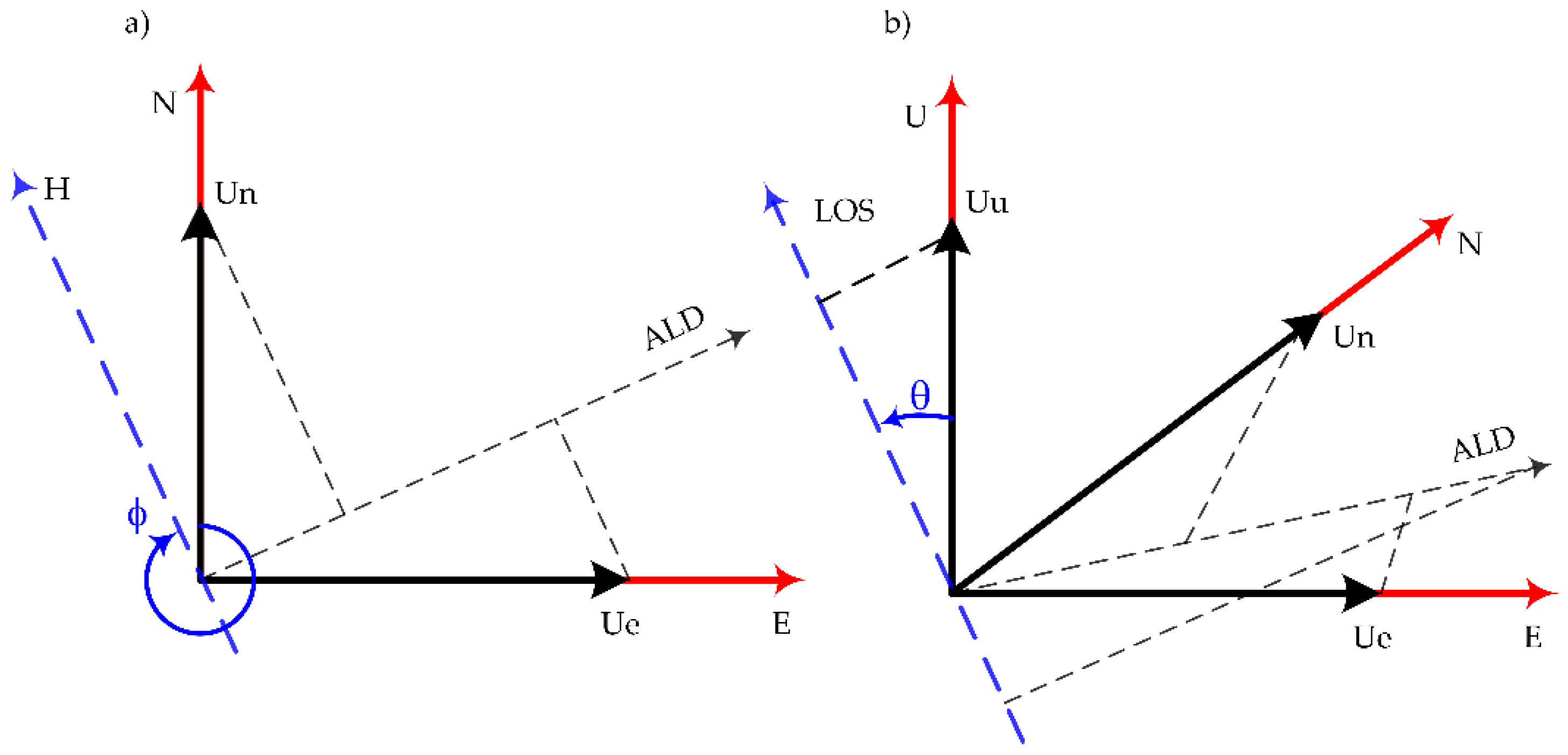
The LOS deformation obtained by InSAR technology does not represent the actual 3D surface deformation, but the projection of the East–West (E), North–South (N), and vertical (U) deformation in the LOS direction [
39]. As shown in
Figure 1,
is the projection of satellite flight direction on the ground,
is the azimuth of satellite flight direction (positive clockwise from the North), and
is the radar incidence angle at the reflection point.
,
, and
are the displacements of three directions of E, N, and U respectively. The relationship between the observed values
and the surface deformation in these three directions can be expressed as [
40]
Equation (1) is the theoretical equation, when
are the observations, and their measurement errors are included at the same time. Let
,
and
, then Equation (1) can be written as
where
,
,
,
is the
ith number of the points (
).
denotes the Kronecker product, and the projection vector
denotes the average of the all points.
The likelihood function between the InSAR LOS displacements
and the 3D displacement
can be described as follows:
where
is the absolute value of the determinant of the variance matrix
.
The GPS stations are interpolated into the spatial density of the LOS observations, and they are regarded as the virtual observations to constrain the 3D displacement field. The expression is showed as
Thus, the prior information constrained on the 3D displacement can be presented by a probability density function (PDF) as
where
, and
is the absolute value of the determinant of the variance matrix
.
According to the Bayesian theorem [
35], the posterior PDF for the 3D displacement is calculated as follows:
where the denominator is a normalizing constant independent of
, which is set as nc. Thus, substituting Equations (4) and (5) into Equation (6):
where
. Based on the maximum a posteriori estimation criterion
, which is equivalent to
where
is the estimation of the
. According to the principle of generalized least squares adjustment [
42], we can obtain the expression of the 3D displacement
2.2. The VOILS Method and its Algorithmic Flow
Although GPS points can coincide with some observation points of InSAR, the spatial density of GPS data points is still not enough, therefore it is necessary to obtain the spatial density consistent with InSAR data points by interpolation. Consequently, this paper uses the ordinary Kriging interpolation method [
43] to interpolate GPS points and obtain the prior initial 3D displacement field at the observation points of InSAR, which is as shown in Equation (5). The 3D displacement field obtained by interpolation inevitably contains errors, therefore, this study designs an iterative least squares for virtual observation, which has the advantages of correcting errors in interpolated GPS displacement and reasonably fusing two types of data. The iteration process is the key step that is different from the traditional method, which is expected to realize the main objectives as described above.
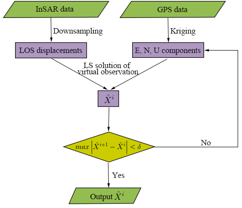
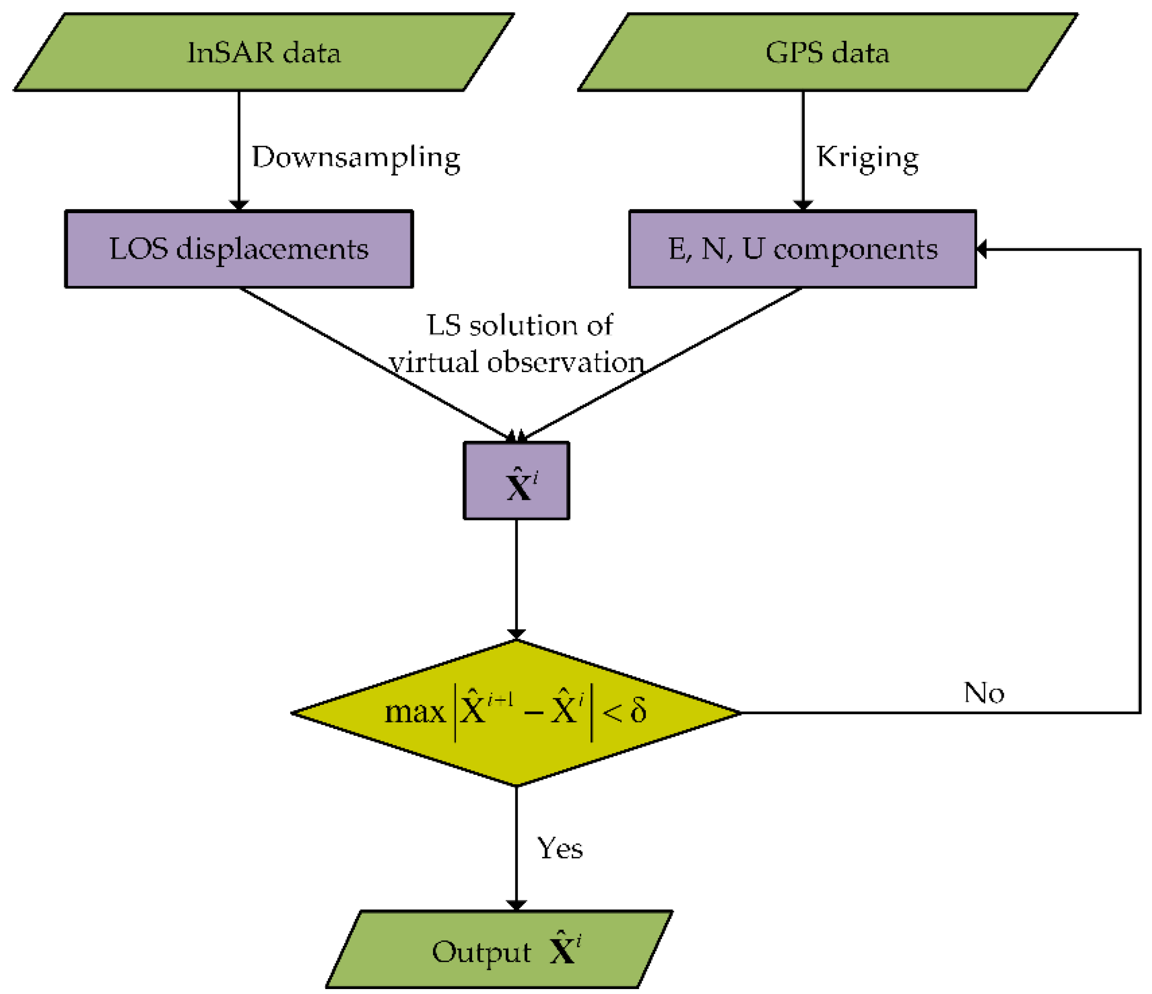
Figure 2 shows the flow chart of the VOILS method. It can be described as: (1) Downsampling InSAR data to obtain sparse LOS displacements; (2) Interpolating GPS data to the spatial density of InSAR downsampled data by the Kriging method as virtual observations; (3) Calculating E, N, and U component’s displacement by the least squares for virtual observation (i.e., Equation (9)); (4) If the maximum absolute value of the difference between the front and back of the 3D displacement is less than the given threshold value δ, the parameter
is the output and the iteration will be terminated, otherwise the virtual observation values E, N, and U will be updated, and the steps 2~4 will repeat.
3. Simulation Experiment
We adopt the following strategies (i.e., uniform and non-uniform) to select GPS observation points. In Scheme 1, we sample the GPS observation points with the uniform mode. To investigate the impact of the different density on the extracted 3D displacement field, 9, 25, 49, and 121 GPS points are selected respectively, which correspond to the spatial resolutions of 30 km, 20 km, 14 km, and 10 km of GPS observation points. In Scheme 2, we employ the non-uniform way to sample the GPS observation points in the displacement field. We use the randperm function in matrix laboratory (MATLAB) to select 9, 25, 49, and 121 points randomly according to the number of uniformly sampled GPS points.
In the comparative analysis of the results, two indicators, i.e., the root mean square error (RMSE) and the percentage of improvement of VOILS method compared with the direct solution method (Per), are used to evaluate the performances of the VOILS method.
(1) RMSE is calculated by the difference
between the fitting value at each grid point and the original simulated true value. The expression is as follows:
where
n means the number of the grid points.
(2) Per, the percentage value of improvement, is presented as follows
where
and
represent the RMSE obtained by the VOILS method and the direct solution method, respectively.
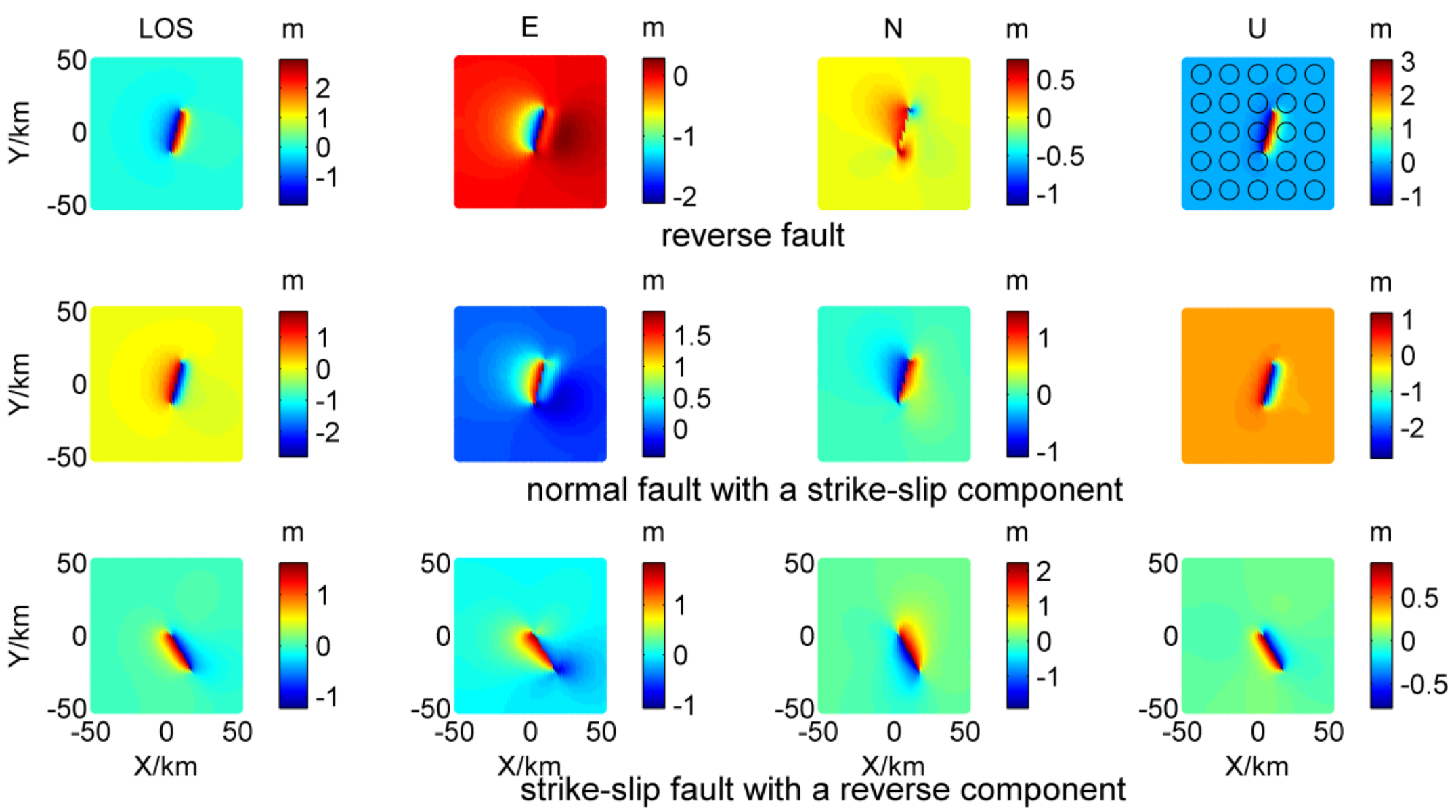
The uniform elastic half-space dislocation theory [
44] is used to simulate the 3D surface displacement field. The deformation area is 100 km × 100 km. The model parameters of reverse fault, normal fault with a strike-slip component, and strike-slip fault with a reverse component are listed in
Table 1. The simulated 3D displacement field is calculated by FORTRAN programs EDGRN/EDCMP [
45].
The simulation field is divided into 51 × 51 grid cells with a 2km interval (see
Figure 3, in which both horizontal and vertical coordinates range from −50 km to 50 km, and the projection coefficient is [Se Sn Su]= [0.340 −0.095 0.935] [
26]). The random errors adhering to normal distribution whose standard deviations are 3 mm, 5 mm, and 30 mm are added to the horizontal component, vertical component, and LOS deformation, respectively. Twenty-five selected points are displayed in the upper right corner subfigure of
Figure 3.
3.1. Experiment with the Reverse Fault
In Scheme 1, we carried out 200 simulation experiments. The RMSE values of the corresponding 3D displacement field are calculated with these two methods, and the results are counted to get the histogram of
Figure 4. It shows the RMSE values of 3D displacement field with different GPS spatial resolutions. It can be seen that the histogram obtained by the VOILS method is closer to the origin of coordinate than that computed by the direct solution method, which implies that the VOILS method exhibits some improvement relative to the direct solution method and can retrieve the 3D displacement field better.
In order to quantitatively illustrate the advantages of the VOILS method and form a more intuitive comparison with the direct solution method, mean improvement percentages for Scheme 1 are listed in
Table 2, which is calculated by Formula (11). It shows that the improvements in all directions are comparable under different GPS spatial resolutions. The improvement degrees of the three directions from high to low are U, E, and N, which may be related to the satellite projection coefficient. The projection coefficients of U, E, and N directions are 0.935, 0.340, and −0.095, respectively. Thus, the vertical direction contributes the most to the LOS deformation, followed by the E and N directions.
The experiments under different GPS spatial resolutions were also carried out. The improved percentages are listed in
Table 1. In addition, the corresponding number of GPS points are listed in brackets. It can be seen that the percentages of improvement display a relatively stable state with the increasing number of GPS points, which indicates that the proposed method has the advantage of not being subject to GPS spatial resolution. Compared with the direct solution method, the percentages of improvement for horizontal directions (i.e., E and N directions) range from 3% to 9%. Unexpectedly, the vertical direction (i.e., U direction) improvement percentage exceeds 68%.
Two hundred simulation experiments were also carried out in Scheme 2, and Per averages are shown in
Table 2. It can be seen that the experiment results from Scheme 2 are similar to those from Scheme 1. Moreover, we executed several random experiments with non-uniformly sampled GPS points and calculated the Per. As shown in
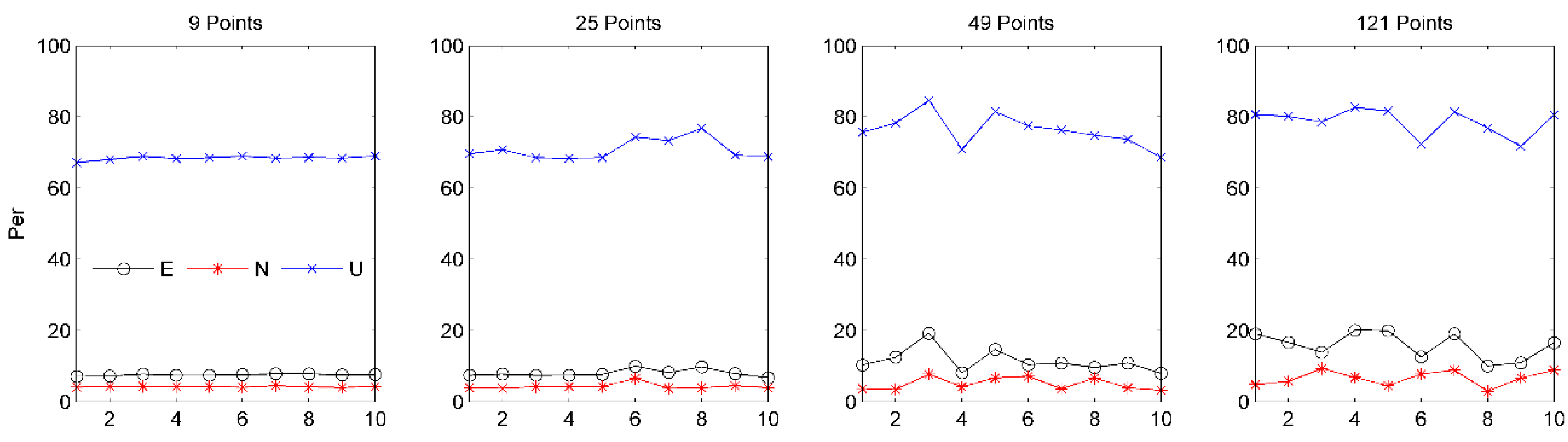
Figure 5, the proposed method in three directions exhibits different degrees of improvement relative to the direct solution method. Evidently, the vertical direction displays obvious improvement. It can be observed that the experimental results show a relatively stable state with the variations of the random sampling GPS points.
3.2. Experiments with the Normal Fault with a Strike-Slip Component and Strike-Slip Fault with a Reverse Component
In the above experiments, the fault slip is assumed to be the reverse fault. The normal fault with a strike-slip component and strike-slip fault with a reverse component will be considered in this section further.
Firstly, we used Scheme 1 and Equation (11) to compute the Per
, as shown in
Table 3. It can be observed that for different types of fault movement, the improvement ratios in different directions under different GPS spatial resolutions are similar. The improvement degrees of three directions from high to low are vertical, E, and N. The results of
Table 3 are similar to the ones of
Table 2. In the case study of the normal fault with a strike-slip component, the improvement ratios of the horizontal direction range from 4% to 8%. Additionally, those of the vertical direction are up to 68%. As for the strike-slip fault with a reverse component, the results show that different directions in improvement ratios demonstrate significant differences. It can be seen that vertical direction has larger improvement ratios exceeding 21%, while lower improvement ratios below 2% occur in the N direction. Despite that, the VOILS method is better than the direct solution method.
Consequently, in Scheme 2, we performed 200 simulated experiments. The Per averages are shown in
Table 3. We found that the results are similar to
Table 2.
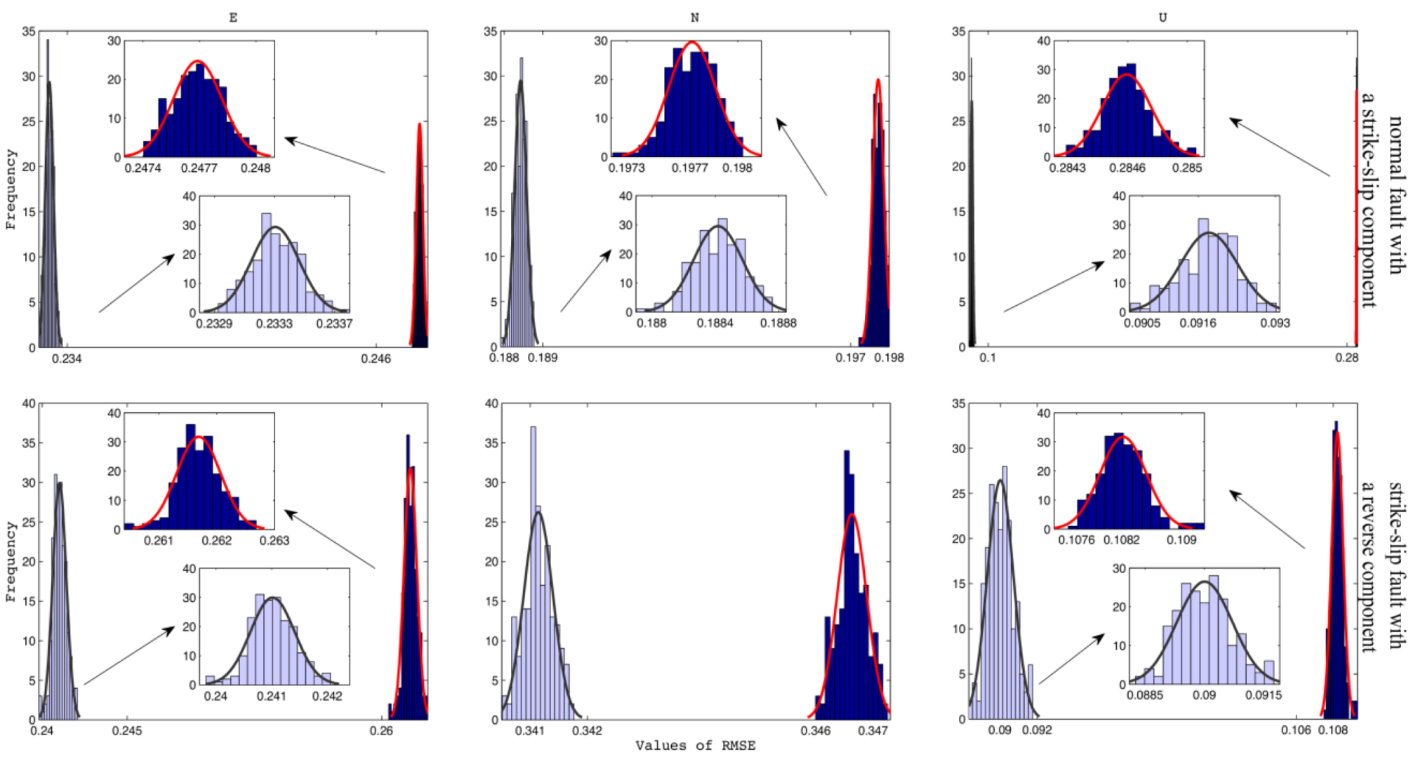
Figure 6 portrays the histogram of RMSE values with a normal density curve at nine non-uniformly sampled GPS points. In addition,
Figure 7 shows the improvement ratio of the VOILS method compared with the direct solution method. Obviously, RMSE values calculated by the VOILS method are smaller than those computed by the direct solution method, which indicates that the VOILS method is better than the direct solution method.
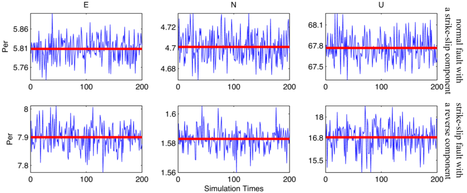
As for the results shown in
Figure 7, the mean Per of the E, N, and U directions for the normal fault with a strike-slip component are 5.81%, 4.70%, and 67.77%, respectively. While those of E, N, and U directions for the strike-slip fault with reverse component are 7.90%, 1.58%, and 16.83%, respectively. From
Table 2 and
Table 3, it can be found that the improvement ratios of the U direction for the strike-slip fault with a reverse component are smaller than those of the reverse fault and normal fault with a strike-slip component. This may be because the slip vector of a strike-slip accompanied by reverse components is mainly in a horizontal direction, while those of a normal fault with a strike-slip component and reverse fault are in a vertical direction. This correlates with the largest contribution of U direction to LOS deformation.
In summary, it is concluded that the improvement degree in the vertical direction is better than that in the horizontal direction. The magnitude of vertical deformation calculated by the VOILS method is closer to the true value than that computed from the direct solution method. This confirms that the VOILS method can make full use of InSAR observations. Our simulation results fully show that the VOILS method is feasible and effective. Furthermore, the proposed method displays obvious advantages in retrieving 3D displacement fields compared to the direct solution method, especially for vertical deformation.
4. 3D Displacement Field Extraction of the Wenchuan Earthquake
4.1. GPS and InSAR Data
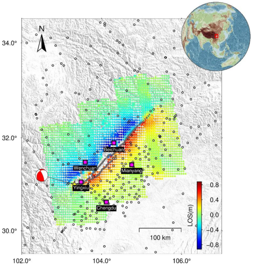
The Wenchuan earthquake occurred on May 12, 2008, on the Longmenshan fault zone in Sichuan Province (
Figure 8). The earthquake caused surface rupture in the Yingxiu–Beichuan fault of the main central fault and the Guanxian–Jiangyou fault of the Qianshan fault [
46]. Previous studies have illustrated that this event is a complex slip mechanism as a variable combination of a reverse and right-lateral component [
46,
47,
48,
49,
50]. After the earthquake, the co-seismic deformation observation data, including GPS data and InSAR data from advanced land observation satellite (ALOS) satellite phased array type L-band synthetic aperture radar (PALSAR) images, were obtained. In this paper, we employed the downsampled 3792 LOS displacements from Xu et al. [
47], and 473 GPS co-seismic displacement data calculated by Wang et al. [
5]. It is noted that 297 GPS points (i.e., 284 campaigned stations and 13 continuous stations) are used in our study, with the spatial distribution of the data shown in
Figure 8.
4.2. Results and Comparative Analysis
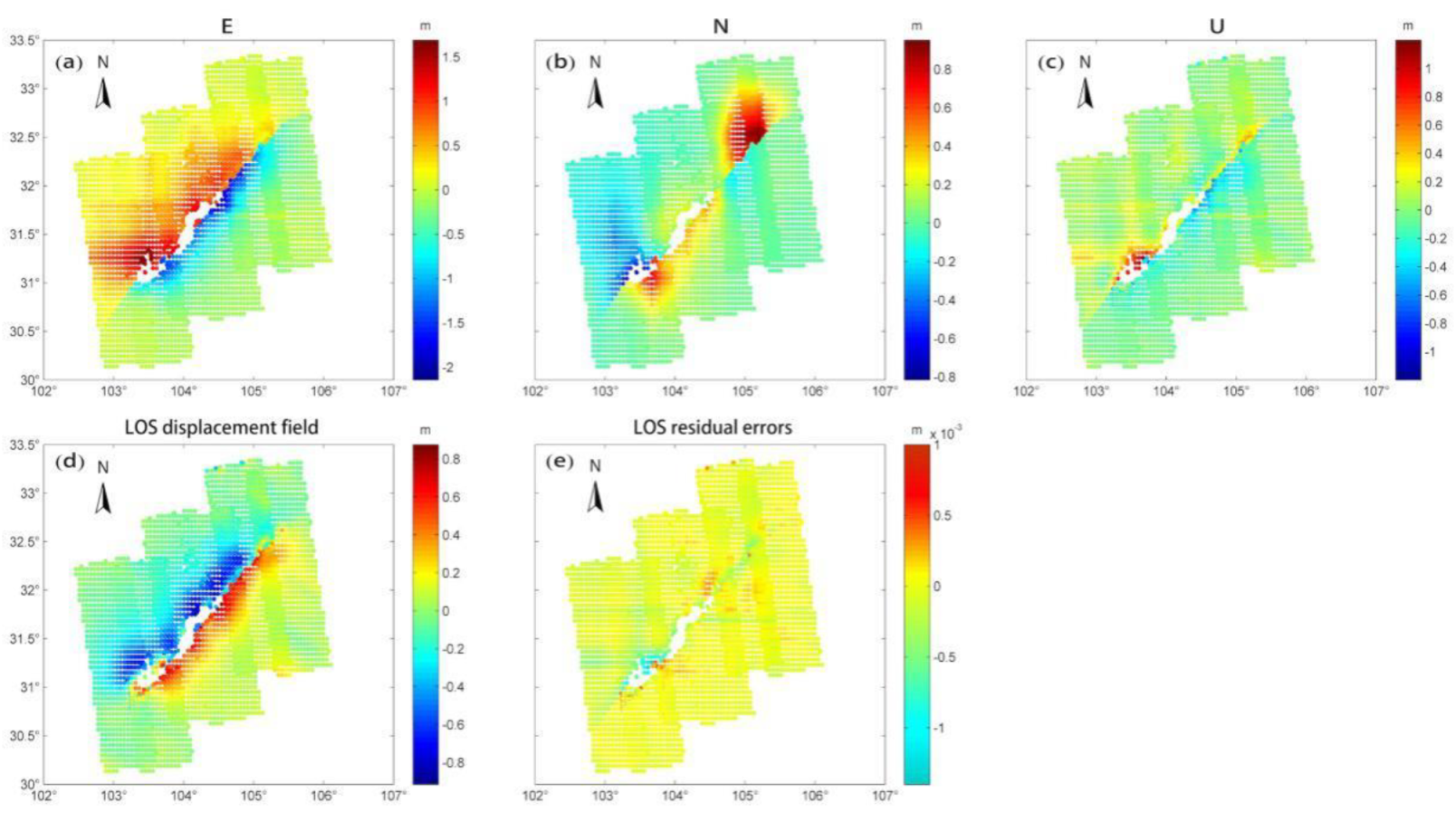
The 3D displacement field of the Wenchuan earthquake obtained by the VOILS method is shown in
Figure 9a–c. Meanwhile, the LOS displacement field and its residual errors are calculated, as shown in
Figure 9d–e.
Figure 9a shows the E direction deformation, and it can be observed that the hanging wall moves eastward with a maximum displacement of 1.69 m, while the footwall moves westward with a maximum displacement of 2.15 m, showing a right-lateral trend. As for the N direction deformation (
Figure 9b), the southwest of the hanging wall moves southward with a maximum displacement of 0.82 m and the northeast section moves northward with a maximum displacement of 0.95 m. The whole footwall moves northward with a maximum displacement of 0.77 m, and the deformation decreases in the northeast direction. The relatively large displacements of the hanging wall and footwall near the epicenter indicate that the reverse component in this area is the largest. Finally, the U direction deformation is shown in
Figure 9c. The hanging wall and footwall near the fault zone appear uplift and subsidence. In addition, the maximum uplift and the maximum subsidence near the epicenter are 1.19 m and 0.95 m respectively, which means that reverse movement existed in the southwest of the fault. The 3D deformation characteristics clearly show the local movement characteristics of the fault and reflect the seismogenic fault’s complexity and heterogeneity.
From
Figure 9d–e, we know that the LOS displacement field is close to that of
Figure 8. Meanwhile, the unit for fitting residual errors after iteration calculation is millimeters, which is at the same order magnitude of the threshold
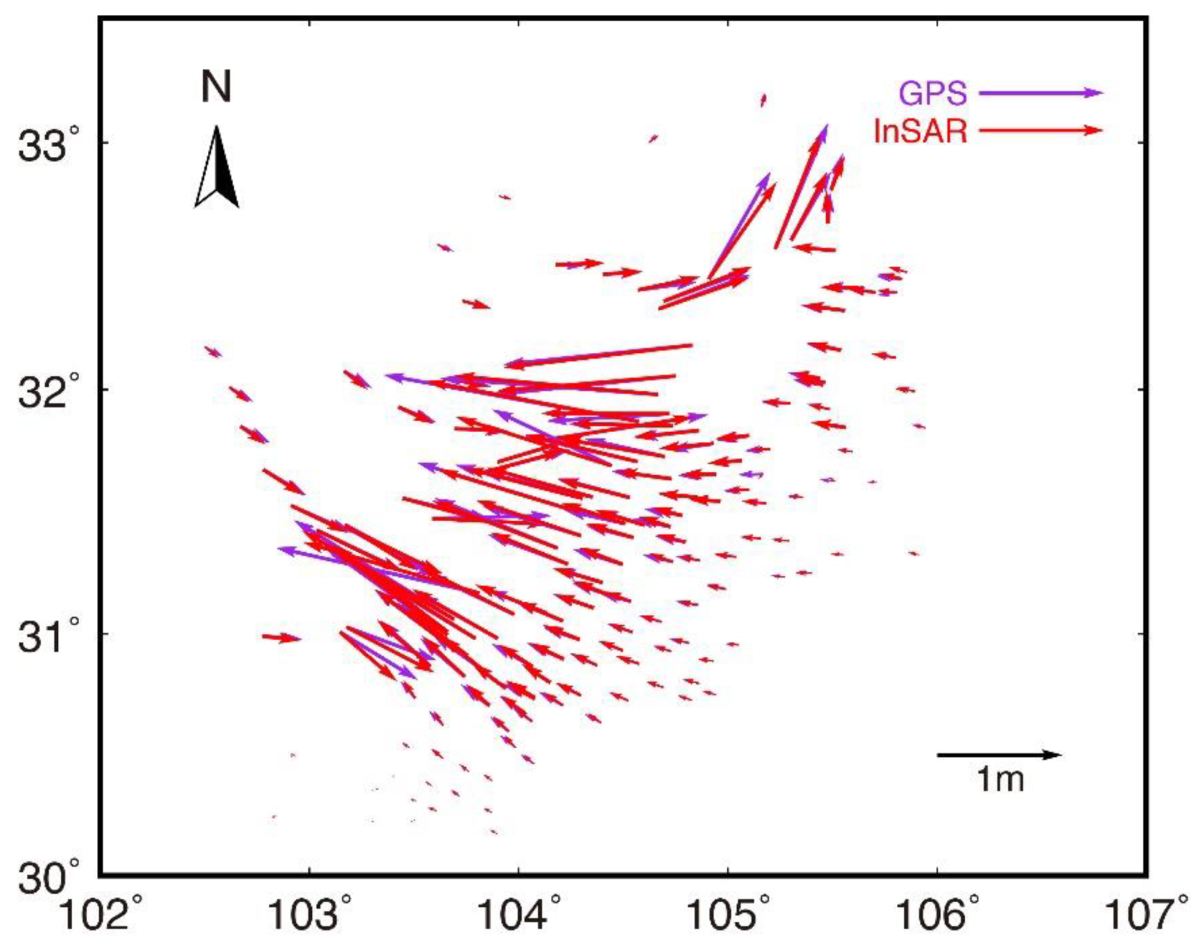
(2 mm) adopted in the iteration process. It is useful to compare the derived coseismic displacement field with independent GPS observations. The InSAR points with a distance of approximately 3 km around the GPS points were chosen for horizontal comparison.
Figure 10 shows the horizontal displacement vectors, indicating that the agreement between the GPS observations and the derived displacements is quite good. The RMSE values between them are 6.1 cm, 2.3 cm, and 5.8 cm in the E, N, and U directions, respectively.
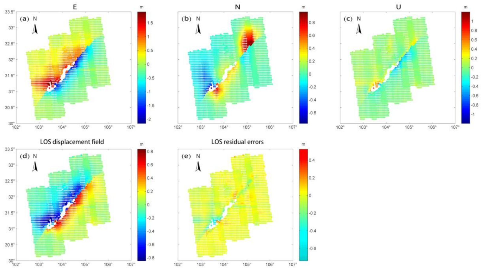
In order to compare with the above results, the 3D displacement field (
Figure 11a–c) was calculated using the direct solution method. The LOS deformation and its residual errors are shown in
Figure 11d–e.
Figure 11a–c show similar features as
Figure 9a–c, while the numerical values are different. It can be seen from
Figure 11e that the residuals along both sides of the seismogenic fault are larger, especially in the southwest of the hanging wall. This can be ascribed to the fault being close to the epicenter, which caused larger deformation, as well as poor interpolation accuracy with less near-field GPS data. This is similar to the characteristic distribution of the LOS deformation residual map produced by Luo et al. [
34]. However, the numerical values are different, which may be related to the data and the method used.
The results indicate that the deformation directions along both sides of the fault are basically opposite, and the larger displacements in the three directions are nearer to the source. Near the epicenter of the E direction, the movement of the hanging wall to the east, relative to the footwall, is dominant, and along the NE direction, the deformation of the hanging wall and footwall is opposite. In the N direction, the northward movement of the northeastern part of the hanging wall is dominant, with a small amount of reverse component. Both the hanging wall and footwall of the U direction have subsidence near the fault zone, and the uplift of the hanging wall is greater than the subsidence of the footwall. In summary, we can understand that the main fault near the epicenter is a reverse fault with a right-lateral strike-slip component, while the northeastern segment is a right-lateral strike-slip with a small amount of reverse component, which is in line with the results of other research [
46,
47,
48,
49,
50].
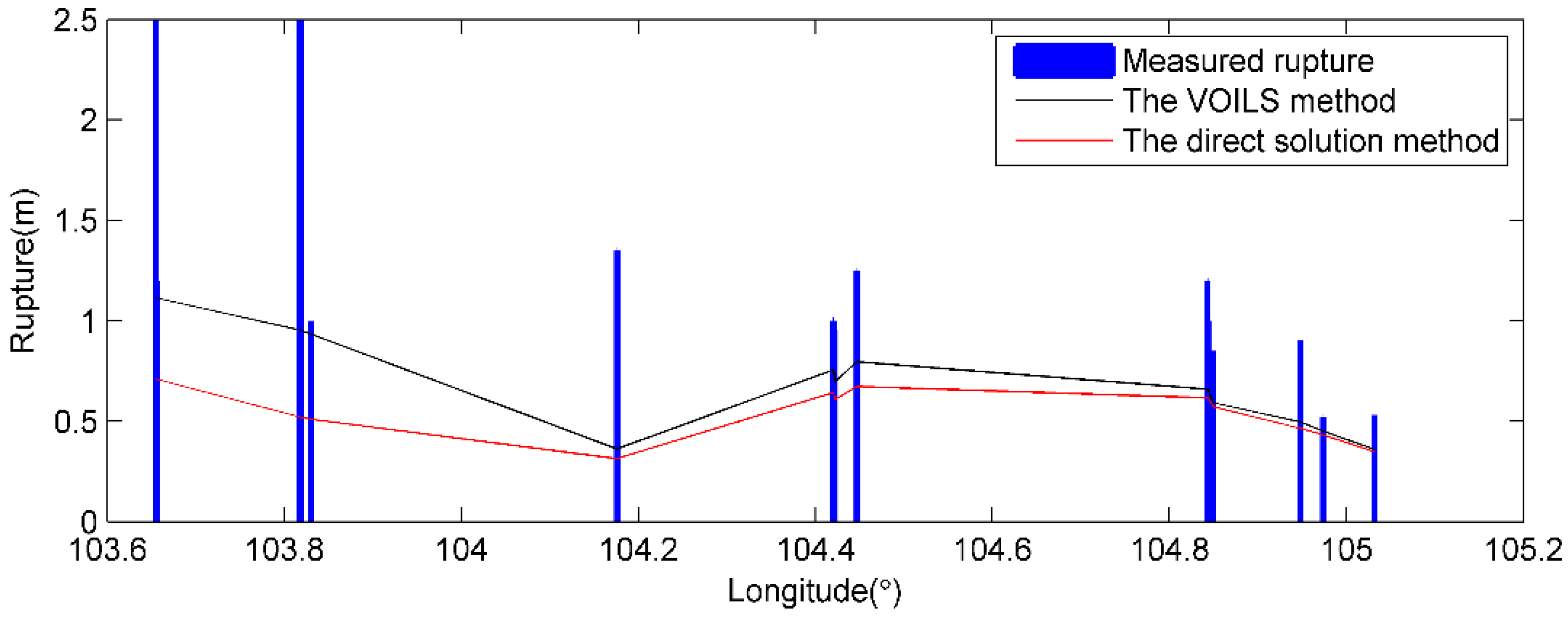
In order to further verify the degree of improvement in the vertical direction, we compared the derived displacements to the surface rupture measurements from Xu et al. (2009) [
50].
Figure 12 shows the comparison of these data. Note that the average displacements of InSAR points with a distance of about 5 km around the field points are used for comparison. It shows that the vertical displacements from the VOILS method are more consistent with the field observations, which indicates that the VOILS method can effectively reduce the impacts of the interpolated errors on parameter estimation to some extent. Meanwhile, these results indicate that the VOILS method performs better than the direct solution method in this event.
Figure 11e shows that the residual magnitude of InSAR is different from that of
Figure 9e. The residual magnitude of InSAR fitted by VOILS method is mm-level, which is significantly smaller than that of the direct solution method. Meanwhile, the results of this study are also different from those of the existing researches [
28,
36,
37,
38]. Therefore, the results obtained by the VOILS method are relatively stable and the fitting is relatively good. On the other hand, the RMSE value of the direct solution method is 0.07m, representing a precision of cm-level. The above analyses show that the VOILS method can make full use of the InSAR observations, and has the ability to exert benefits from GPS and InSAR data.
5. Conclusions
In the conventional direct solution method, GPS data need to be interpolated first, which will undoubtedly introduce errors. Therefore, this paper proposes the VOILS method, which can correct the errors in GPS 3D deformation interpolation, and realize the reasonable fusion of GPS/InSAR observations in 3D displacement extraction based on the iteration process, making better use of InSAR data and calculating relatively stable 3D displacement fields.
In the simulation examples, uniform and non-uniform schemes are adopted to select GPS points. In the uniform sampling scheme, the spatial resolutions of GPS points of 30 km, 20 km, 14 km, and 10 km were considered. Accompanied with the comprehensive analyses of the reverse fault, normal fault with a strike-slip component, and strike-slip fault with a reverse component, it demonstrates that the VOILS method is better than the direct solution method in both horizontal and vertical directions. From the results of the uniform sampling scheme, we see that the percentages of improvement for the reverse fault are approximately 3~9% and 70%, for the normal fault with a strike-slip component approximately 4~8% and 68%, and for the strike-slip fault with a reverse component approximately 1~8% and 22%. Moreover, the degree of improvement in the vertical direction is more obvious. The simulation experiments show that the VOILS method can make better use of the InSAR observations, and has feasibility and validity.
The VOILS method was applied to get the 3D displacement field of the 2008 Wenchuan earthquake. The LOS residual magnitude obtained by the VOILS method is mm-level, while the magnitude of the direct solution method is cm-level. Furthermore, the results of the VOILS method are relatively stable. Based on the analyses of 3D deformation, it can be seen that the mechanism of the main shock was mainly a reverse motion with a right-lateral strike-slip component. In the northeast of the fault, the mechanism is dominated by the right-lateral strike-slip. In particular, the comparison with the rupture displacements from the field investigations shows that the VOILS method is better than the direct solution method.
Author Contributions
Conception and the design of the experiments, C.X. and Y.L.; the performance of the experiments, L.X.; formal analysis, L.X., Y.L., C.X. Y.W. and J.F.; writing—original draft preparation, L.X.; writing—review and editing, L.X., C.X., Y.L., Y.W. and J.F.; supervision, C.X. All authors have read and agreed to the published version of the manuscript.
Funding
This work is co-supported by the National Key Research Development Program of China under Grant No. 2018YFC1503603, No. 2018YFC1503604, and the National Natural Science Foundation of China under Grant No. 41721003, No. 41874011, and No. 41774011.
Acknowledgments
The authors thank academic editor and anonymous reviewers for their comments and constructive suggestions, which highly improved the quality of the manuscript. Thanks are also given to Guangyu Xu for helping drawing and Hanqing Chen for helping polish this manuscript. The ALOS SAR data were provided by JAXA. Some figures were plotted by the Generic Mapping Tools software [
51].
Conflicts of Interest
The authors declare no conflict of interest.
References
- Massonnet, D.; Rossi, M.; Carmona, C.; Adragna, F.; Peltzer, G.; Feigl, K.L.; Rabaute, T. The displacement field of the Landers earthquake mapped by radar interferometry. Nature 1993, 364, 138–142. [Google Scholar] [CrossRef]
- Wright, T.J. Toward mapping surface deformation in three dimensions using InSAR. Geophys. Res. Lett. 2004, 31, 169–178. [Google Scholar] [CrossRef]
- Xu, G.; Xu, C.; Wen, Y. Sentinel-1 observation of the 2017 Sangsefid earthquake, northeastern Iran: Rupture of a blind reserve-slip fault near the Eastern Kopeh Dagh. Tectonophysics 2018, 731, 131–138. [Google Scholar] [CrossRef]
- Shen, Z.-K.; Sun, J.; Zhang, P.; Wan, Y.; Wang, M.; Bürgmann, R.; Zeng, Y.; Gan, W.; Liao, H.; Wang, Q. Slip maxima at fault junctions and rupturing of barriers during the 2008 Wenchuan earthquake. Nat. Geosci. 2009, 2, 718–724. [Google Scholar] [CrossRef]
- Wang, Q.; Qiao, X.J.; Lan, Q.G.; Freymueller, J.T. Rupture of deep faults in the 2008 Wenchuan earthquake and uplift of the Longmen Shan. Nat. Geosci. 2011, 4, 634–640. [Google Scholar]
- Fang, J.; Xu, C.; Wen, Y.; Wang, S.; Xu, G.; Zhao, Y.; Yi, L. The 2018 Mw 7.5 Palu earthquake: A supershear rupture event constrained by InSAR and broadband regional seismograms. Remote Sens. 2019, 11, 1330. [Google Scholar] [CrossRef]
- Wang, S.; Xu, C.; Wen, Y.; Yin, Z.; Jiang, G.; Fang, L. Slip model for the 25 November 2016 Mw 6.6 Aketao earthquake, western China, revealed by Sentinel-1 and ALOS-2 observations. Remote Sens. 2017, 9, 325. [Google Scholar] [CrossRef]
- He, P.; Wen, Y.; Xu, C.; Chen, Y. Complete three-dimensional near-field surface displacements from imaging geodesy techniques applied to the 2016 Kumamoto earthquake. Remote Sens. Environ. 2019, 232, 111321. [Google Scholar] [CrossRef]
- Muller, C.; Del Potro, R.; Biggs, J.; Gottsmann, J.; Ebmeier, S.K.; Guillaume, S.; Cattin, P.-H.; Van Der Laat, R. Integrated velocity field from ground and satellite geodetic techniques: Application to Arenal volcano. Geophys. J. Int. 2015, 200, 861–877. [Google Scholar] [CrossRef]
- Palano, M.; Puglisi, G.; Gresta, S. Ground deformation patterns at Mt. Etna from 1993 to 2000 from joint use of InSAR and GPS techniques. J. Volcanol. Geoth. Res. 2008, 169, 99–120. [Google Scholar] [CrossRef]
- Guo, Q.; Xu, C.; Wen, Y.; Liu, Y.; Xu, G. The 2017 noneruptive unrest at the Caldera of Cerro Azul Volcano (Galápagos Islands) revealed by InSAR observations and geodetic modelling. Remote Sens. 2019, 11, 1992. [Google Scholar] [CrossRef]
- Pritchard, M.; Biggs, J.; Wauthier, C.; Sansosti, E.; Arnold, D.W.D.; Delgado, F.; Ebmeier, S.K.; Henderson, S.T.; Stephens, K.; Cooper, C.; et al. Towards coordinated regional multi-satellite InSAR volcano observations: Results from the Latin America pilot project. J. Appl. Volcanol. 2018, 7, 5. [Google Scholar] [CrossRef]
- Bonì, R.; Meisina, C.; Cigna, F.; Herrera, G.; Notti, D.; Bricker, S.; McCormack, H.; Tomás, R.; Béjar-Pizarro, M.; Mulas, J.; et al. Exploitation of satellite A-DInSAR time series for detection, characterization and modelling of land subsidence. Geosciences 2017, 7, 25. [Google Scholar]
- Bonì, R.; Herrera, G.; Meisina, C.; Notti, D.; Béjar-Pizarro, M.; Zucca, F.; Gonzalez, P.J.; Palano, M.; Tomás, R.; Fernandez, J.; et al. Twenty-year advanced DInSAR analysis of severe land subsidence: The Alto Guadalentín Basin (Spain) case study. Eng. Geol. 2015, 198, 40–52. [Google Scholar] [CrossRef]
- Caló, F.; Notti, D.; Galve, J.; Abdikan, S.; Görüm, T.; Pepe, A.; Balik Şanli, F. DInSAR-based eetection of land subsidence and correlation with groundwater depletion in Konya Plain, Turkey. Remote Sens. 2017, 9, 83. [Google Scholar] [CrossRef]
- Cheloni, D.; Serpelloni, E.; Devoti, R.; D’Agostino, N.; Pietrantonio, G.; Riguzzi, F.; Anzidei, M.; Avallone, A.; Cavaliere, A.; Cecere, G.; et al. GPS observations of coseismic deformation following the 2016, August 24, Mw 6 Amatrice earthquake (central Italy): Data, analysis and preliminary fault model. Ann. Geophys. 2016, 59. [Google Scholar] [CrossRef]
- Jiang, Z.; Huang, D.; Yuan, L.; Hassan, A.; Zhang, L.; Yang, Z. Coseismic and postseismic deformation associated with the 2016 Mw 7.8 Kaikoura earthquake, New Zealand: Fault movement investigation and seismic hazard analysis. Earth Planets Space 2018, 70, 62. [Google Scholar] [CrossRef]
- Houlié, N.; Dreger, D.; Kim, A. GPS source solution of the 2004 Parkfield earthquake. Sci. Rep. 2014, 4, 3646. [Google Scholar] [CrossRef]
- Johanson, I.A.; Fielding, E.J.; Rolandone, F.; Buμrgmann, R. Coseismic and postseismic slip of the 2004 Parkfield earthquake from space-geodetic data. Bull. Seismol. Soc. Am. 2006, 96, S269–S282. [Google Scholar] [CrossRef]
- Murray, J. Slip on the San Andreas Fault at Parkfield, California, over two earthquake cycles, and the implications for seismic hazard. Bull. Seismol. Soc. Am. 2006, 96, S283–S303. [Google Scholar] [CrossRef]
- Liu, P.; Custodio, S.; Archuleta, R.J. Kinematic Inversion of the 2004 M 6.0 Parkfield Earthquake Including an Approximation to Site Effects. Bull. Seismol. Soc. Am. 2006, 96, S143–S158. [Google Scholar] [CrossRef]
- Delouis, B.; Nocquet, J.-M.; Vallée, M. Slip distribution of the February 27, 2010 Mw = 8.8 Maule Earthquake, central Chile, from static and high-rate GPS, InSAR, and broadband teleseismic data. Geophys. Res. Lett. 2010, 37. [Google Scholar] [CrossRef]
- Palano, M.; Viccaro, M.; Zuccarello, F.; Gresta, S. Magma transport and storage at Mt. Etna (Italy): A review of geodetic and petrological data for the 2002–03, 2004 and 2006 eruptions. J. Volcanol. Geoth. Res. 2017, 347, 149–164. [Google Scholar] [CrossRef]
- Owen, S.; Segall, P.; Lisowski, M.; Miklius, A.; Murray, M.; Bevis, M.; Foster, J. 30 January 1997 eruptive event on Kilauea Volcano, Hawaii, as monitored by continuous GPS. Geophys. Res. Lett. 2000, 27, 2757–2760. [Google Scholar] [CrossRef]
- Gudmundsson, S.; Gudmundsson, M.T.; Björnsson, H.; Sigmundsson, F.; Rott, H.; Carstensen, J.M. Three-dimensional glacier surface motion maps at the Gja´lp eruption site, Iceland, inferred from combining InSAR and other ice-displacement data. Ann. Glaciol. 2002, 34, 315–322. [Google Scholar] [CrossRef]
- Samsonov, S.; Tiampo, K. Analytical optimization of a DInSAR and GPS dataset for derivation of three-dimensional surface motion. IEEE Geosci. Remote Sens. Lett. 2006, 3, 107–111. [Google Scholar] [CrossRef]
- Samsonov, S.; Tiampo, K.; Rundle, J.; Li, Z. Application of DInSAR-GPS optimization for derivation of fine-scale surface motion maps of southern California. IEEE Trans. Geosci. Remote Sens. 2007, 45, 512–521. [Google Scholar] [CrossRef]
- Song, X.G.; Shen, X.; Jiang, Y.; Wan, J.-H. Coseismic 3D deformation field acquisition of the Wenchuan earthquake based on InSAR and GPS data. Seismol. Geol. 2015, 37, 222–231. (In Chinese) [Google Scholar]
- Luo, H.; Chen, T. Three-dimensional surface displacement field associated with the 25 April 2015 Gorkha, Nepal, earthquake: Solution from integrated InSAR and GPS measurements with an extended SISTEM approach. Remote Sens. 2016, 8, 559. [Google Scholar] [CrossRef]
- Guo, Z.; Wen, Y.; Xu, G.; Wang, S.; Wang, X.; Liu, Y.; Xu, C. Fault slip model of the 2018 Mw 6.6 Hokkaido eastern Iburi, Japan, earthquake estimated from satellite Radar and GPS measurements. Remote Sens. 2019, 11, 1667. [Google Scholar] [CrossRef]
- Hu, J. Theory and Method of Estimating Three-Dimensional Displacement with InSAR Based on the Modern Surveying Adjustment. Ph.D. Thesis, Central South University, Changsha, China, 2013. [Google Scholar]
- Guglielmino, F.; Nunnari, G.; Puglisi, G.; Spata, A. Simultaneous and integrated strain tensor estimation from geodetic and satellite deformation measurements to obtain three-dimensional displacement maps. IEEE Trans. Geosci. Remote Sens. 2011, 49, 1815–1826. [Google Scholar] [CrossRef]
- Song, X.; Jiang, Y.; Shan, X.; Qu, C. Deriving 3D coseismic deformation field by combining GPS and InSAR data based on the elastic dislocation model. Int. J. Appl. Earth Obs. Geoinf. 2017, 57, 104–112. [Google Scholar] [CrossRef]
- Luo, H.; Liu, Y.; Chen, T.; Xu, C.; Wen, Y. Derivation of 3-D surface deformation from an integration of InSAR and GNSS measurements based on Akaike’s Bayesian Information Criterion. Geophys. J. Int. 2016, 204, 292–310. [Google Scholar] [CrossRef]
- Bagnardi, M.; Hooper, A. inversion of surface deformation data for rapid estimates of source parameters and uncertainties: A Bayesian approach. Geochem. Geophy. Geosy. 2018, 19, 2194–2211. [Google Scholar] [CrossRef]
- Ban, B.S.; Wu, J.C.; Chen, Y.Q.; Feng, G.C.; Hu, S.C. Calculation of three-dimensional terrain deformation of Wenchuan earthquake with GPS and InSAR data. J. Geod. Geodyn. 2010, 30, 25–28. (In Chinese) [Google Scholar]
- Xu, K.K.; Niu, Y.F.; Wu, J.C. Establishment of 3-D coseismic terrain displacement field with GPS and InSAR. J. Geod. Geodyn 2014, 34, 15–18. (In Chinese) [Google Scholar]
- Shan, X.J.; Qu, C.Y.; Guo, L.M.; Zhang, G.-H.; Song, X.; Zhang, G.; Wen, S.-Y.; Wang, C.; Xu, X.-B.; Liu, Y.-H. The vertical coseismic deformation field of the Wenchuan earthquake based on the combination of GPS and InSAR measurements. Seismol. Geol. 2014, 36, 718–730. (In Chinese) [Google Scholar]
- He, X.F.; He, M. InSAR Earth Observation Data Processing and Comprehensive Measuring; Science Press: Beijing, China, 2012; p. 210. [Google Scholar]
- Fuhrmann, T.; Garthwaite, M.C. Resolving three-dimensional surface motion with InSAR: Constraints from multi-geometry data fusion. Remote Sens. 2019, 11, 241. [Google Scholar] [CrossRef]
- Wen, Y.M. Coseismic and Postseismic Deformation Using Synthetic Aperture Radar Interferometry. Ph.D. Thesis, Wuhan University, Wuhan, China, 2009. [Google Scholar]
- Cui, X.Z.; Yu, Z.C.; Tao, B.Z.; Liu, D.; Yu, Z.; Sun, H.; Wang, X. Generalized Surveying Adjustment, 2nd ed.; Wuhan University Press: Wuhan, China, 2009; p. 21. [Google Scholar]
- Gudmundsson, S.; Sigmundsson, F.; Carstensen, J.M. Three-dimensional surface motion maps estimated from combined interferometric synthetic aperture radar and GPS data. J. Geophys. Res. 2002, 107, 2250. [Google Scholar] [CrossRef]
- Okada, Y. Surface deformation due to shear and tensile faults in a half-space. Bull. Seismol. Soc. Am. 1985, 75, 1135–1154. [Google Scholar]
- Wang, R.; Martín, F.L.; Roth, F. Computation of deformation induced by earthquakes in a multi-layered elastic crust—FORTRAN programs EDGRN/EDCMP. Comp. Geosci. 2003, 29, 195–207. [Google Scholar] [CrossRef]
- Xu, X.W.; Wen, X.Z.; Ye, J.Q.; Ma, B.Q. The Ms 8.0 Wenchuan earthquake surface ruptures and its seismogenic structure. Seismol. Geol 2008, 30, 597–629. (In Chinese) [Google Scholar]
- Xu, C.; Liu, Y.; Wen, Y.; Wang, R.-Q. Coseismic slip distribution of the 2008 Mw 7.9 Wenchuan earthquake from joint inversion of GPS and InSAR data. Bull. Seismol. Soc. Am. 2010, 100, 2736–2749. [Google Scholar] [CrossRef]
- Zhang, G.H.; Qu, C.Y.; Song, X.G. Slip distribution and source parameters inverted from co-seismic deformation derived by InSAR technology of Wenchuan Mw 7.9 earthquake. Chin. J. Geophys. 2010, 53, 269–279. (In Chinese) [Google Scholar]
- Shan, X.J.; Qu, C.Y.; Song, X.G.; Zhang, G.F. Coseismic surface deformation caused by the Wenchuan Ms 8.0 earthquake from InSAR data analysis. Chin. J. Geophys. 2009, 52, 496–504. (In Chinese) [Google Scholar]
- Xu, X.; Wen, X.; Yu, G.; Chen, G.; Klinger, Y.; Hubbard, J.; Shaw, J. Coseismic reverse- and oblique-slip surface faulting generated by the 2008 Mw 7.9 Wenchuan earthquake, China. Geology 2009, 37, 515–518. [Google Scholar] [CrossRef]
- Wessel, P.; Smith, W.H.F. New, improved version of generic mapping tools released. Eos Trans. Am. Geophys. Union 1998, 79, 579. [Google Scholar] [CrossRef]
Figure 1.
Sketch map of the relationship between interferometric synthetic aperture radar (InSAR) observation and surface displacements [
41]. (
a) Top-view showing the North–South (N) and East–West (E) components projection on the azimuth look direction (ALD). (
b) 3D sketch of surface deformation components and InSAR observations.
Figure 2.
Flow chart of the iterative least squares for virtual observation.
Figure 2.
Flow chart of the iterative least squares for virtual observation.
Figure 3.
Simulated line of sight (LOS) displacement field and 3D displacement field for three types of faults. (The first line is a reverse fault. The second one is a normal fault with a strike-slip component. The last one is a strike-slip fault with a reverse component.).
Figure 3.
Simulated line of sight (LOS) displacement field and 3D displacement field for three types of faults. (The first line is a reverse fault. The second one is a normal fault with a strike-slip component. The last one is a strike-slip fault with a reverse component.).
Figure 4.
Root mean square error (RMSE) values with a normal density curve histogram for the reverse fault of Scheme 1. (The black normal density curve is the result of the iterative least squares for virtual observation (VOILS) method. The red one is the direct solution method, and the small figure in each subfigure is the local enlarged image of the original image).
Figure 5.
The variation of improvement percentages for Scheme 2 under different global positioning system (GPS) points.
Figure 5.
The variation of improvement percentages for Scheme 2 under different global positioning system (GPS) points.
Figure 6.
Root mean square error (RMSE) values with a normal density curve histogram under nine global positioning system (GPS) points for Scheme 2.
Figure 6.
Root mean square error (RMSE) values with a normal density curve histogram under nine global positioning system (GPS) points for Scheme 2.
Figure 7.
The improvement ratios of the VOILS method compared with the direct solution method under nine global positioning system (GPS) points for Scheme 2.
Figure 7.
The improvement ratios of the VOILS method compared with the direct solution method under nine global positioning system (GPS) points for Scheme 2.
Figure 8.
The tectonic setting map of the Wenchuan earthquake. The color-shaded dots denote the LOS displacements from the advanced land observation satellite (ALOS) satellite phased array type L-band synthetic aperture radar (PALSAR) images. Open circles denote the GPS stations. The yellow star depicts the epicenter of the 2008 Wenchuan earthquake, and the red bench ball denotes the focal mechanism solution from the U.S. Geological Survey (USGS). The gray lines denote the rupture traces of this event. The magenta rectangles represent the locations of surrounding cities.
Figure 9.
The results obtained by the VOILS method, (a), (b), and (c) are the deformations of E, N, and vertical (U) directions, respectively. (d) is the modelled LOS displacement field. (e) are the residual errors between the modelled and observed LOS displacements.
Figure 9.
The results obtained by the VOILS method, (a), (b), and (c) are the deformations of E, N, and vertical (U) directions, respectively. (d) is the modelled LOS displacement field. (e) are the residual errors between the modelled and observed LOS displacements.
Figure 10.
The coseismic horizontal displacements. The purple arrows show the horizontal displacement vectors derived from the GPS observations, and the red arrows denote the vectors from the derived horizontal displacement.
Figure 10.
The coseismic horizontal displacements. The purple arrows show the horizontal displacement vectors derived from the GPS observations, and the red arrows denote the vectors from the derived horizontal displacement.
Figure 11.
The results obtained by the direct solution method, (a), (b), and (c) are the deformations of E, N, and U directions, respectively. (d) is the modelled LOS displacement field. (e) are the residual errors between the modelled and observed LOS displacements.
Figure 11.
The results obtained by the direct solution method, (a), (b), and (c) are the deformations of E, N, and U directions, respectively. (d) is the modelled LOS displacement field. (e) are the residual errors between the modelled and observed LOS displacements.
Figure 12.
Comparison of the derived vertical displacements with the surface rupture measurements (The blue bar represents the measured rupture from field investigations (Xu et al., 2009) [
50]. The black and red lines represent the displacements by making subtraction between the derived deformation on hanging wall and footwall from the VOILS method and the direct solution method, respectively.).
Table 1.
Model parameters of reverse fault, normal fault with a strike-slip component and strike-slip fault with a reverse component.
Table 1.
Model parameters of reverse fault, normal fault with a strike-slip component and strike-slip fault with a reverse component.
| Type | X
(km) | Y
(km) | Depth
(km) | Length
(km) | Width (km) | Slip
(m) | Strike
(°) | Dip
(°) | Rake
(°) |
|---|
| reverse fault | 0 | −15 | 0 | 30 | 10 | 5 | 15 | 60 | 90 |
| normal fault with a strike-slip component | 0 | −15 | 0 | 30 | 10 | 5 | 15 | 60 | −70 |
| strike-slip fault with a reverse component | 0 | 0 | 0 | 30 | 10 | 5 | 150 | 85 | 20 |
Table 2.
The Per in the reverse fault for two schemes.
Table 2.
The Per in the reverse fault for two schemes.
| Scheme | E (%) | N (%) | U (%) | GPS spatial resolution (No.) |
|---|
| Scheme 1
| 8.68 | 5.16 | 68.86 | 30 km × 30 km (9) |
| 7.79 | 4.41 | 69.48 | 20 km × 20 km (25) |
| 7.93 | 4.33 | 69.55 | 14 km × 14 km (49) |
| 7.89 | 4.03 | 69.21 | 10 km × 10 km (121) |
| 8.17 | 4.74 | 69.56 | 30 km × 20 km (15) |
| 8.44 | 4.90 | 69.88 | 30 km × 10 km (33) |
| 8.53 | 4.95 | 70.13 | 30 km × 6 km (91) |
| 7.92 | 4.38 | 70.17 | 20 km × 10 km (55) |
| 7.93 | 4.34 | 70.68 | 20 km × 6 km (105) |
| 7.80 | 4.18 | 69.82 | 14 km × 10 km (77) |
| 7.78 | 4.10 | 70.34 | 14 km × 6 km (119) |
| 7.91 | 3.88 | 69.72 | 10 km × 6 km (187) |
| Scheme 2
| 7.13 | 4.05 | 67.17 | 9 |
| 7.41 | 3.95 | 69.65 | 25 |
| 8.10 | 4.17 | 70.93 | 49 |
| 10.96 | 6.65 | 71.76 | 121 |
Table 3.
The Per in the normal fault with a strike-slip component and strike-slip fault with a reverse component for two schemes.
Table 3.
The Per in the normal fault with a strike-slip component and strike-slip fault with a reverse component for two schemes.
| Scheme | Type | E (%) | N (%) | U (%) | GPS spatial resolution (No.) |
|---|
| Scheme 1
| normal fault with a strike-slip component | 7.22 | 4.79 | 68.01 | 30 km × 30 km (9) |
| 5.99 | 4.80 | 68.63 | 20 km × 20 km (25) |
| 6.18 | 4.86 | 68.56 | 14 km × 14 km (49) |
| 6.15 | 4.80 | 68.29 | 10 km × 10 km (121) |
| strike-slip fault with a reverse component | 7.78 | 1.51 | 21.15 | 30 km × 30 km (9) |
| 7.93 | 1.53 | 22.12 | 20 km × 20 km (25) |
| 7.99 | 1.55 | 22.36 | 14 km × 14 km (49) |
| 7.97 | 1.54 | 22.55 | 10 km × 10 km (121) |
| Scheme 2
| normal fault with a strike-slip component | 5.81 | 4.70 | 67.77 | 9 |
| 6.32 | 5.09 | 72.61 | 25 |
| 11.30 | 5.07 | 76.81 | 49 |
| 9.74 | 4.60 | 76.07 | 121 |
| strike-slip fault with a reverse component | 7.90 | 1.58 | 16.83 | 9 |
| 7.84 | 1.42 | 23.33 | 25 |
| 7.78 | 1.55 | 18.17 | 49 |
| 9.41 | 1.81 | 25.96 | 121 |
© 2020 by the authors. Licensee MDPI, Basel, Switzerland. This article is an open access article distributed under the terms and conditions of the Creative Commons Attribution (CC BY) license (http://creativecommons.org/licenses/by/4.0/).


