Earth Observation for the Implementation of Sustainable Development Goal 11 Indicators at Local Scale: Monitoring of the Migrant Population Distribution

 ,
,  ,
,  ,
,
Abstract
1. Introduction
2. Materials and Methods
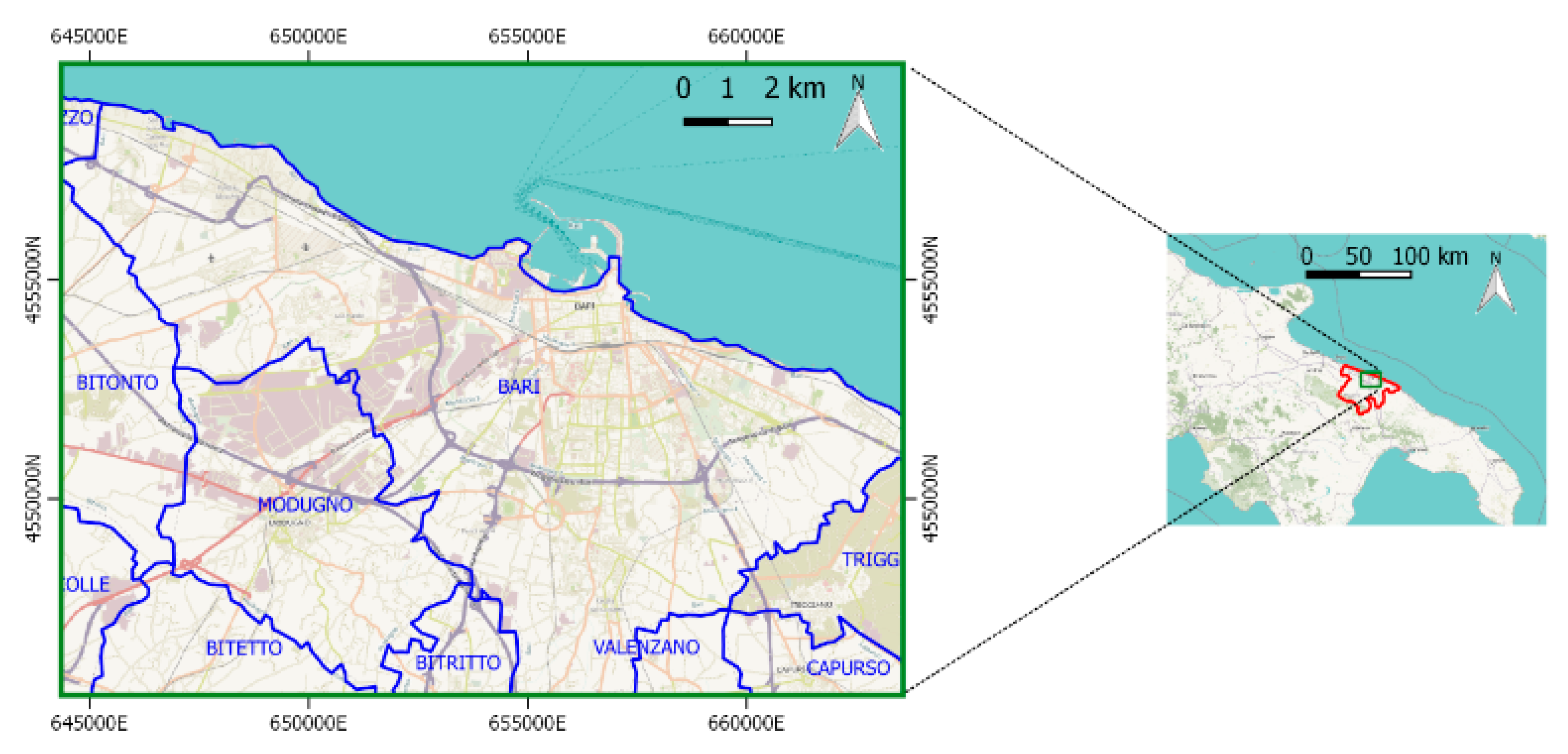
2.1. Study Area
2.2. Satellite Derived Products
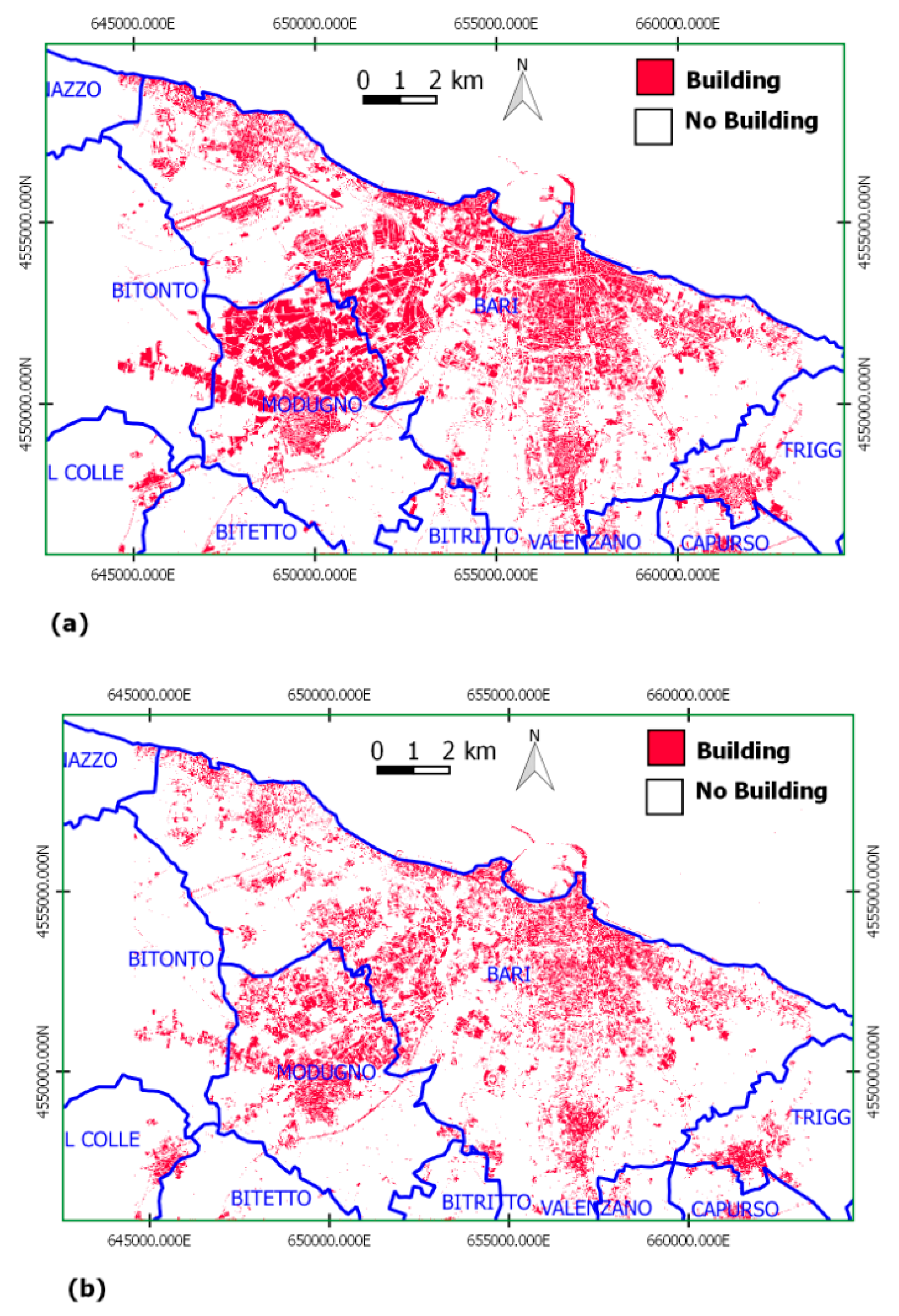
- Data-driven pixel-based approach. A pixel-based Support Vector Machine (SVM) classifier [25] was applied as a data-driven classifier, with a Radial Basis Function (RBF) kernel. The 10 image spectral bands were fed as input to the classifier along with the slope measurement from a Digital Elevation Model (DEM) available at 8 m. The latter input was added as input for discriminating built-up objects from extraction sites. The final following classes were considered: B15/A1 (Artificial Structures/Built Up); B15/A2A6 (Artificial Structures/Extraction sites); (B27 or B28)/A1 (Artificial or Natural Waterbodies/Water); A11/(A1 or A2)A9 or A12/(A3 or A4)E1 (Cultivated Lands or Natural Vegetation/(Trees or Shrubs) Evergreen); A11/(A1 or A2)A10 or A12/(A3 or A4) E2 (Cultivated Lands or Natural Vegetation/(Trees or Shrubs)Deciduous); A12/A2 (Natural Vegetation/Herbaceous); A11/A3 (Cultivated Lands/Herbaceous. The output LC map was produced by training the SVM classifier with 11,965 reference pixels. Next, the freely available [26], 5 m-buffered road map, dated 2018, was used in order to discriminate buildings from roads within the B15/A1 output map layer (built-up).
- Knowledge-driven object-based approach includes two different steps: a preliminary segmentation and a successive classification [27]. The hierarchical scheme adopted by the FAO–LCCS taxonomy was implemented for class discrimination. First, Vegetated or Not-Vegetated objects (LCCS Level 1) and then, for each one, Terrestrial or Aquatic areas, were recognized (LCCS Level 2). Finally, within the Artificial Structures layer, buildings were discriminated from roads using the Length/Width morphological feature. The latter exploits the elongated dominant shape that characterizes roads but not buildings.
2.3. Updated Statistical Census Data: Collection and Harmonization
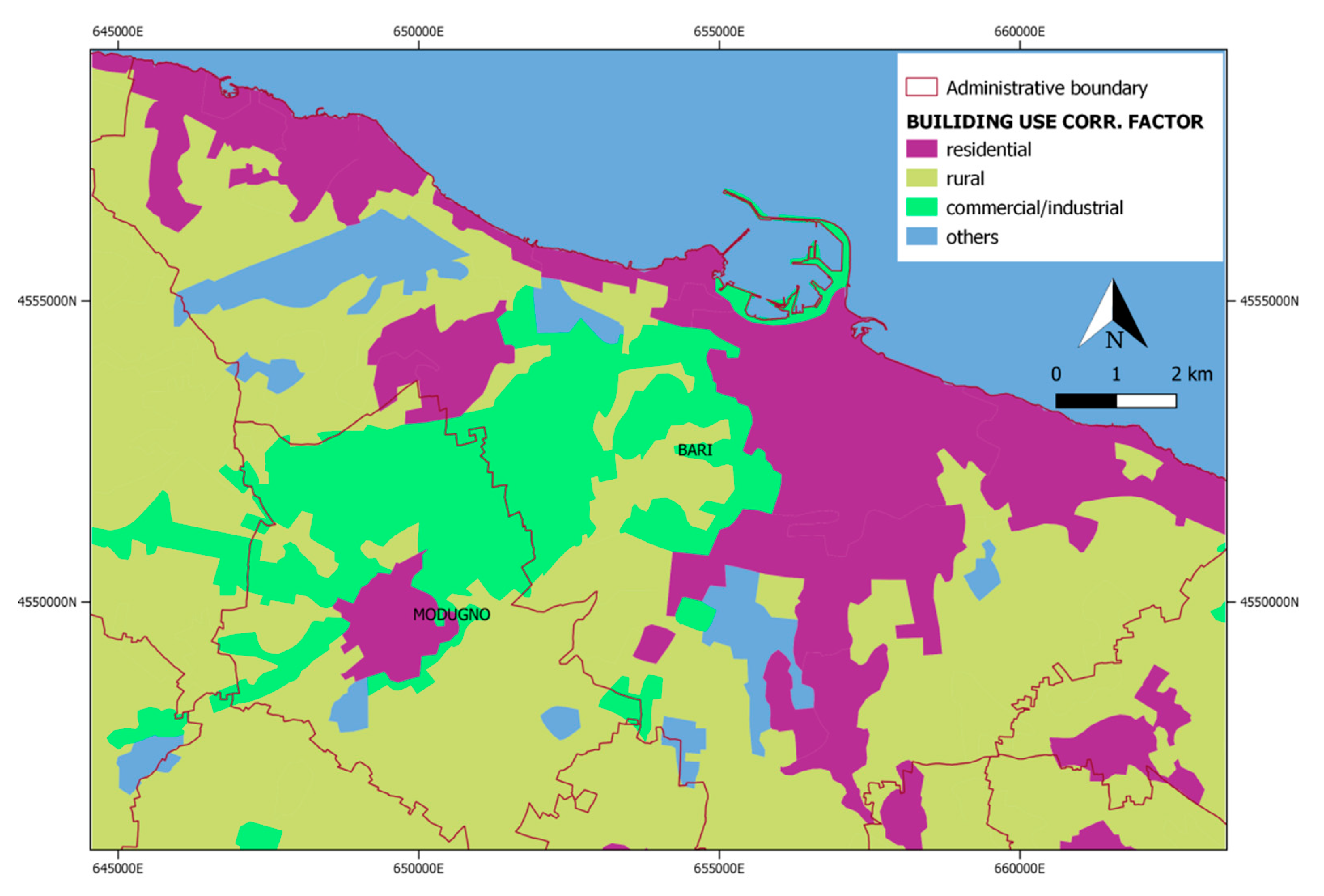
2.4. Building Use Information
2.5. Ancillary Data for the Implementation of SDG 11 Subindicators
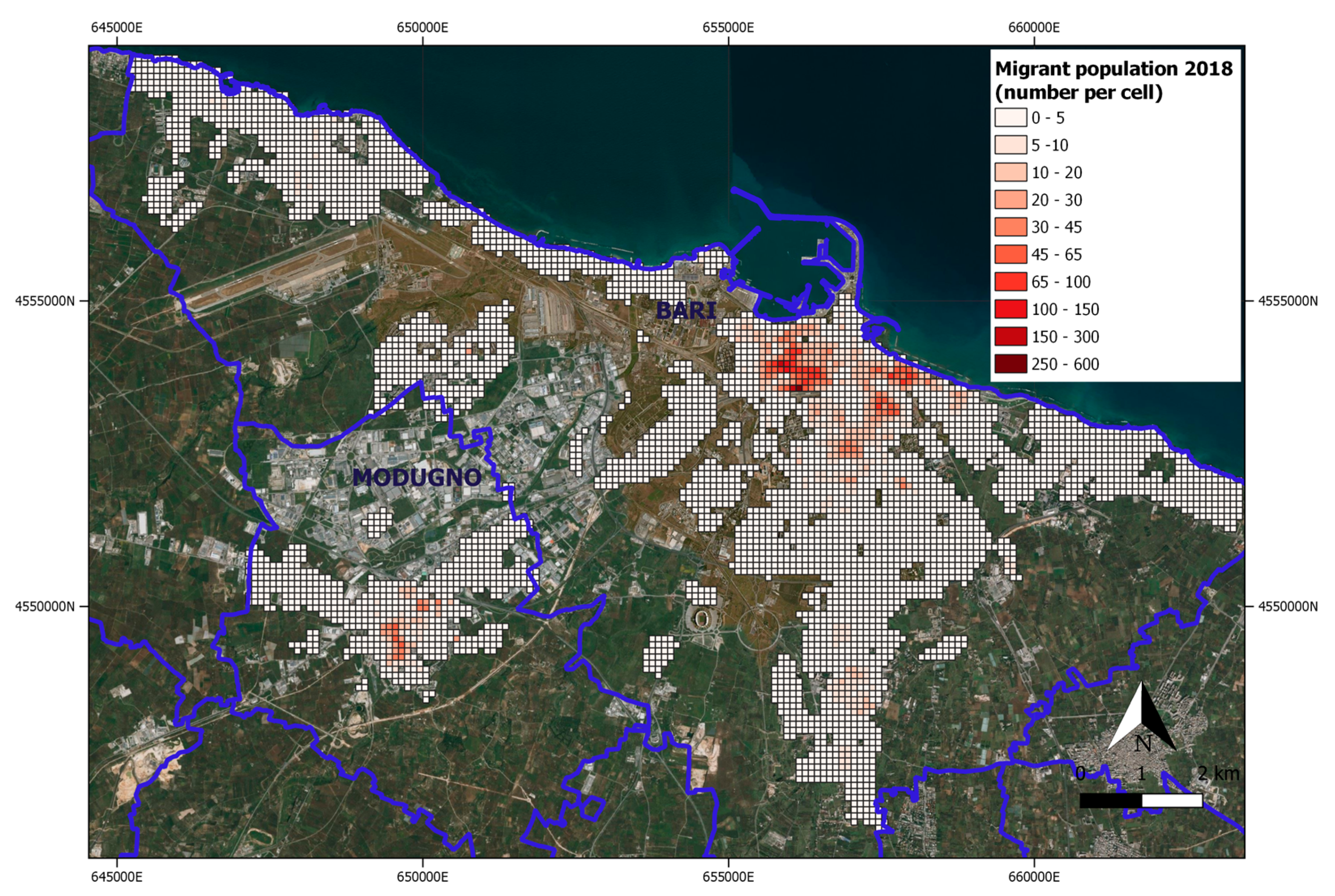
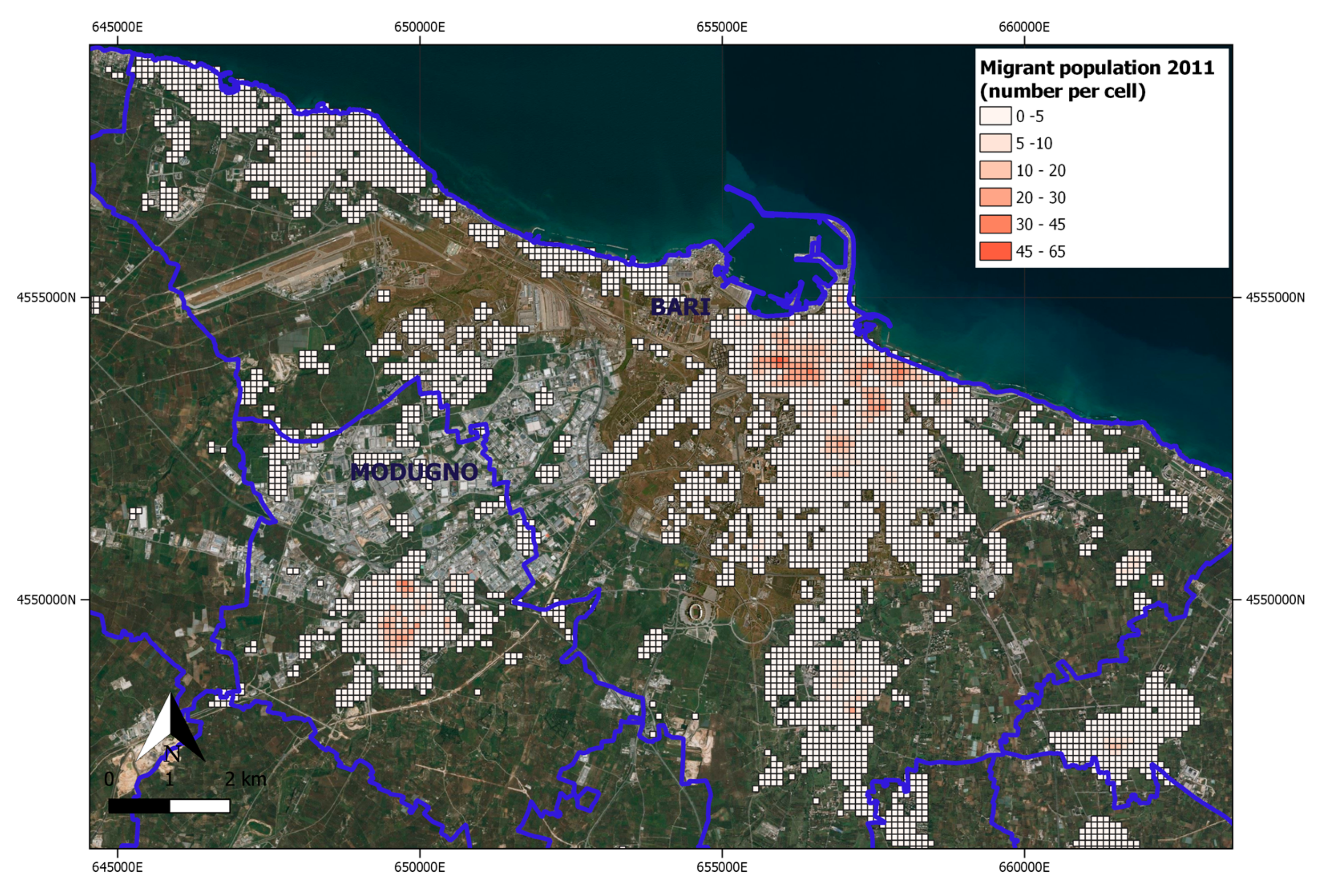
2.6. Updating Spatial Distribution of Resident Migrant Population: the Dasymetric Mapping Method
2.7. SDG Indicators Implementation
3. Results
3.1. Classification of Sentinel-2 Imagery
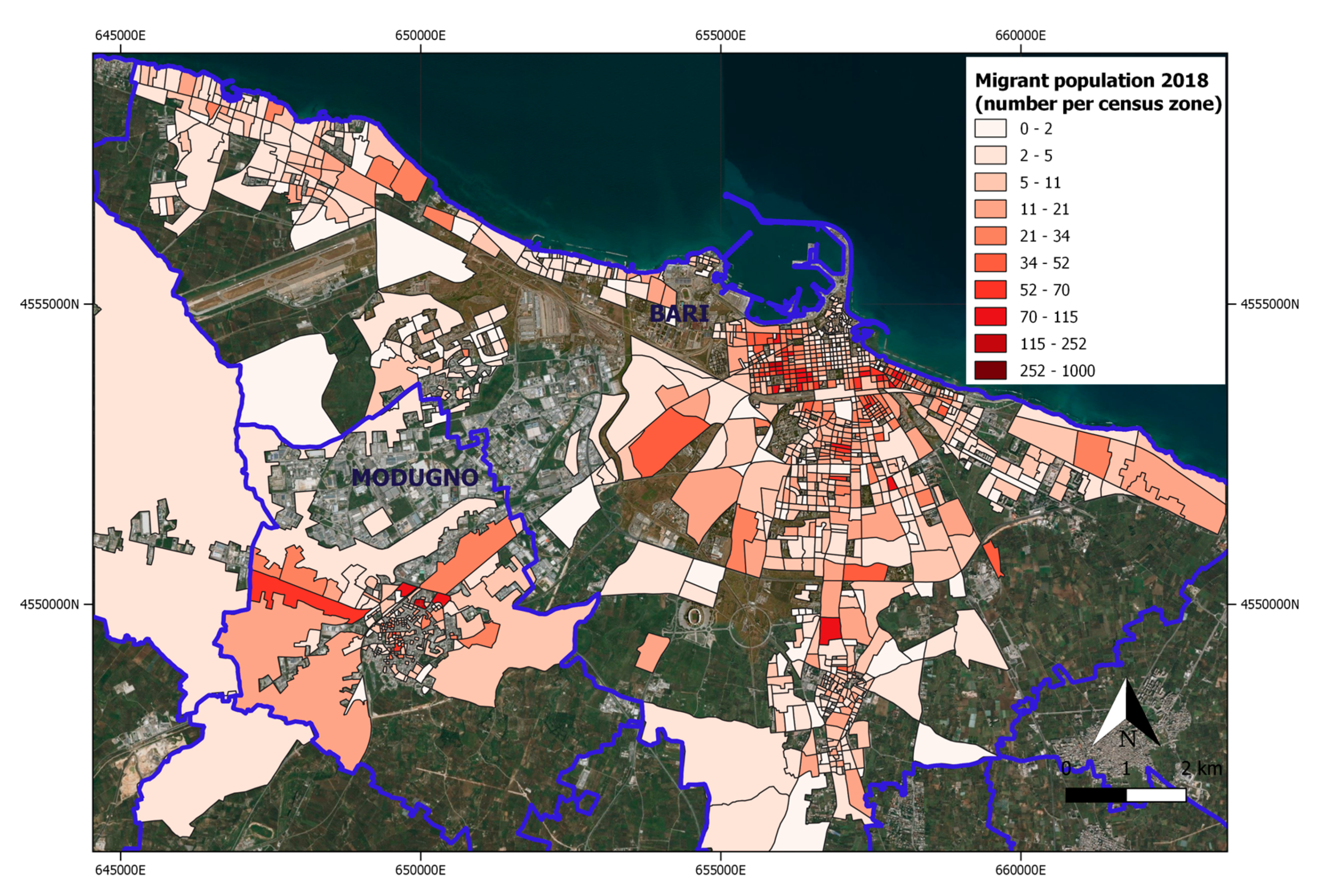
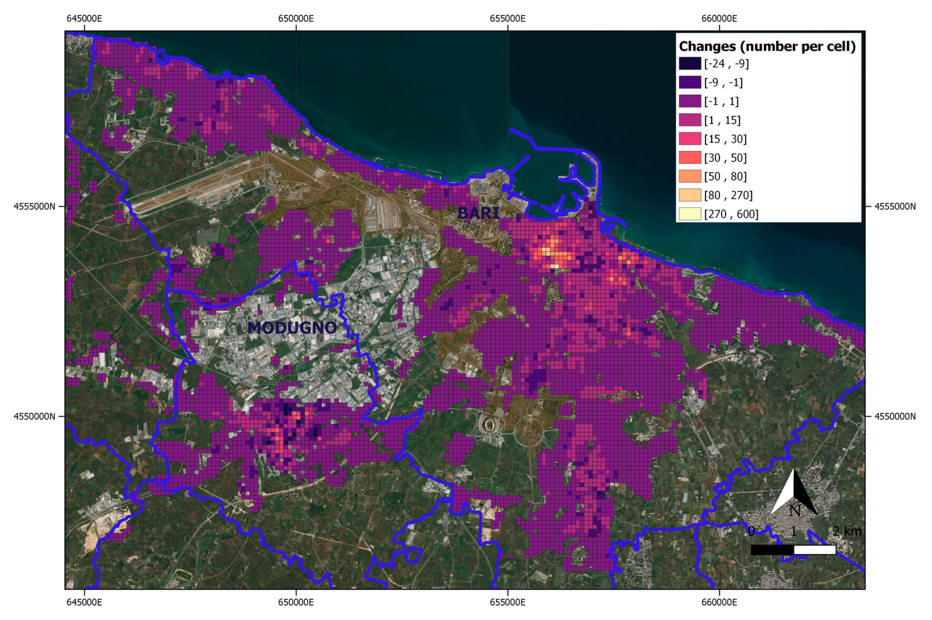
3.2. Regular Migrant Population Map Updating
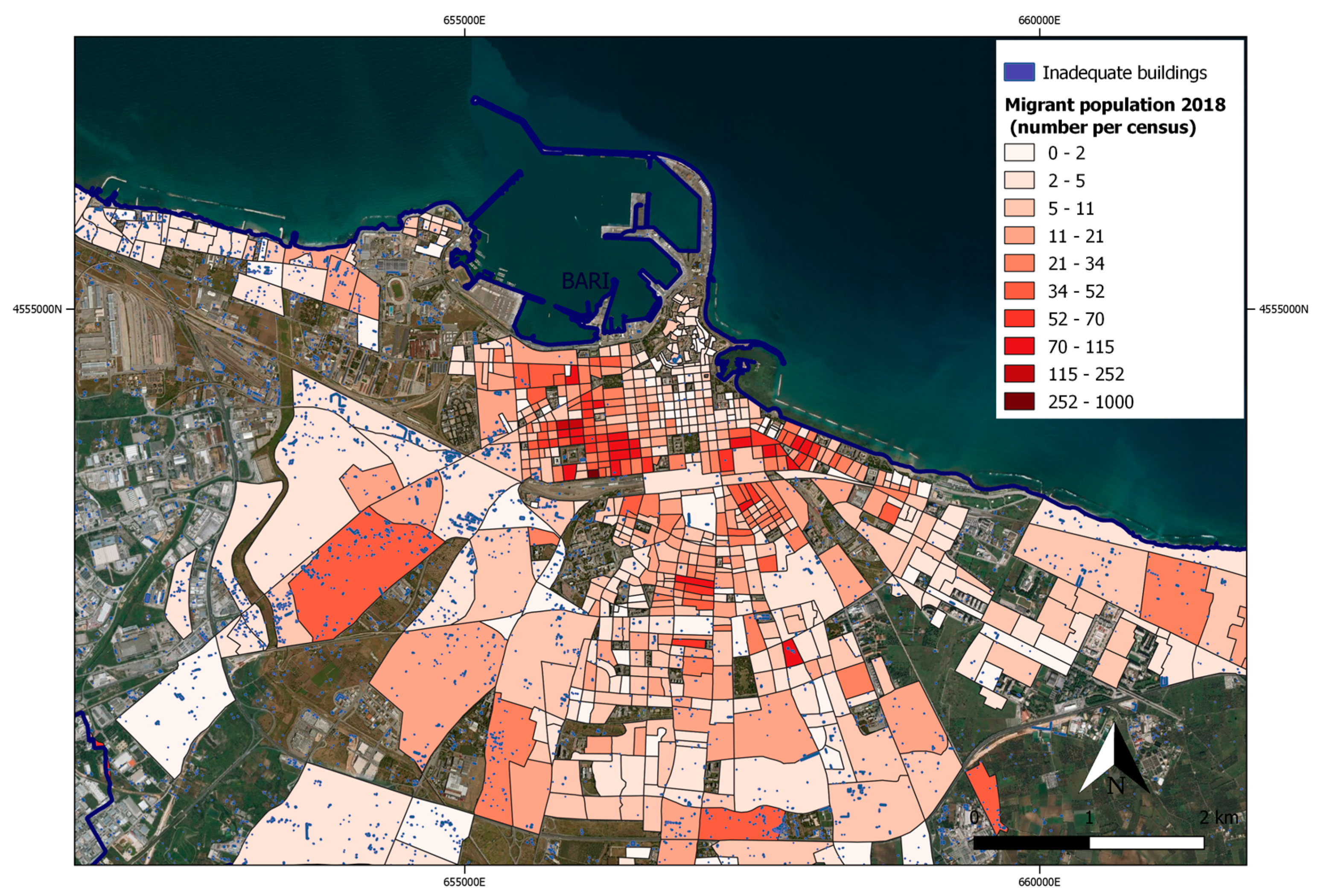
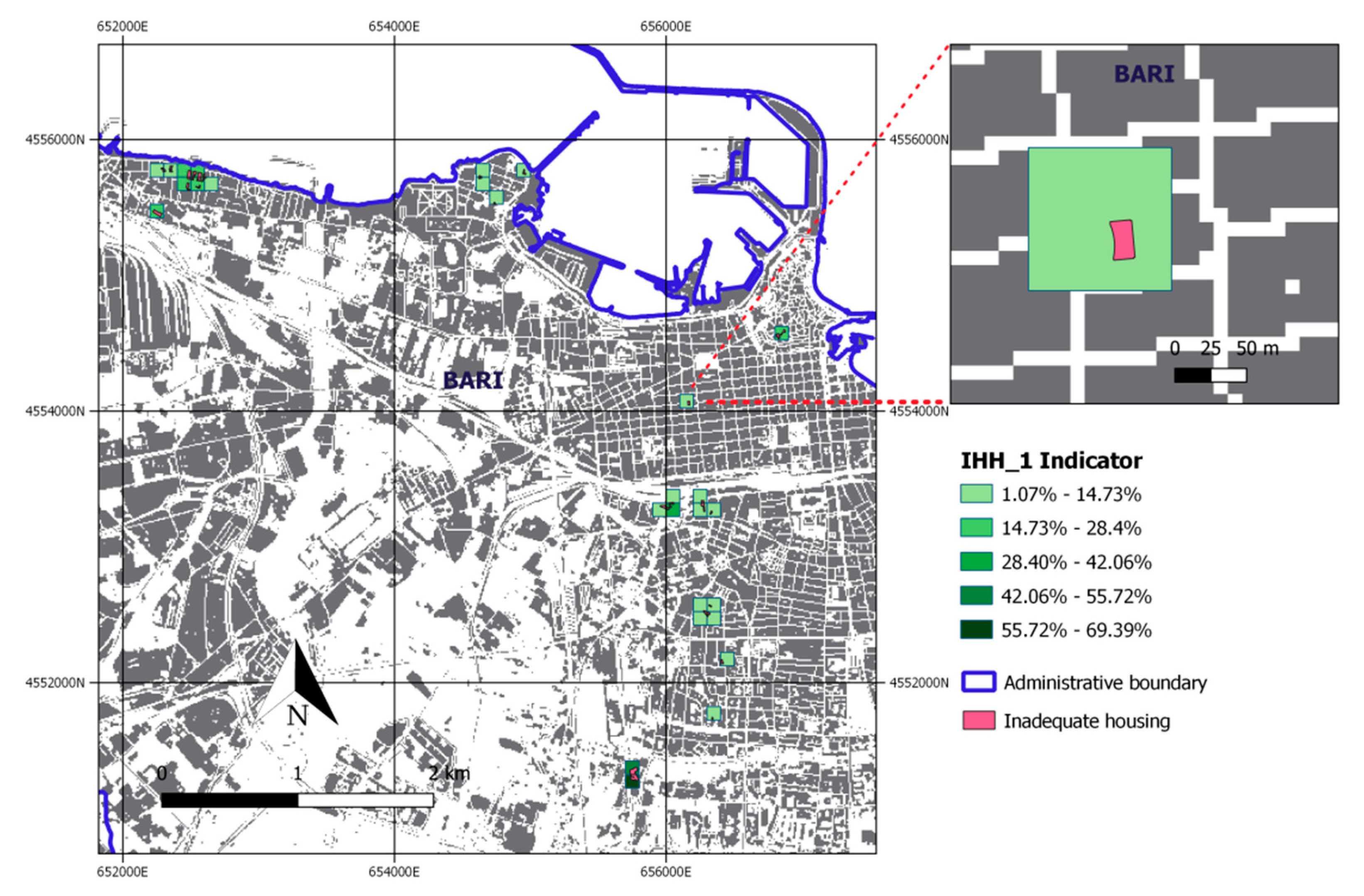
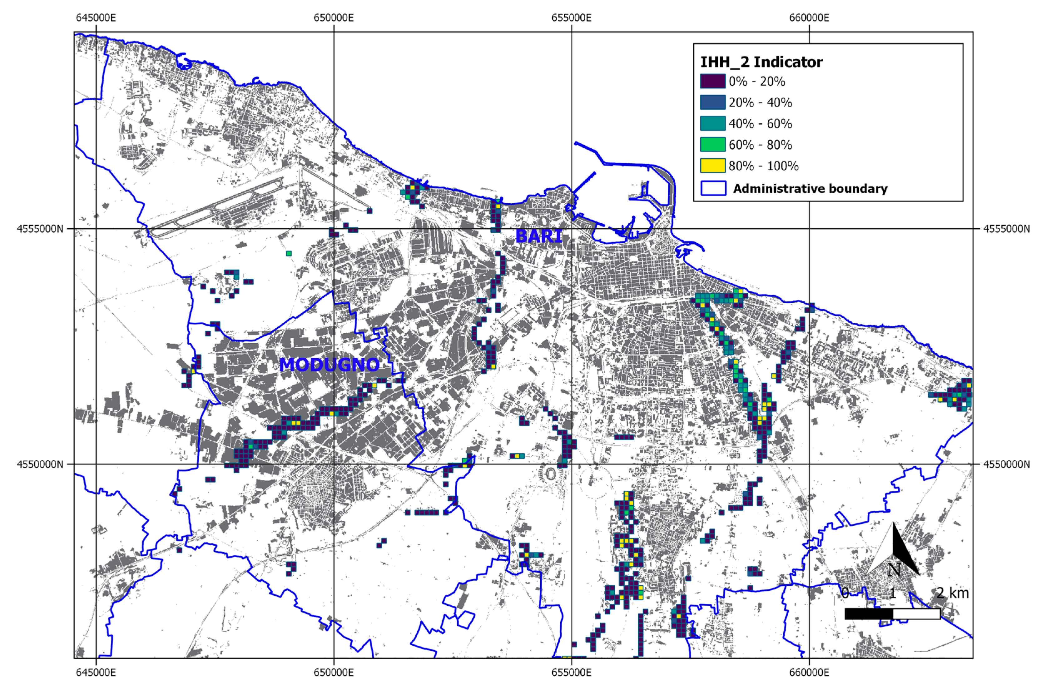
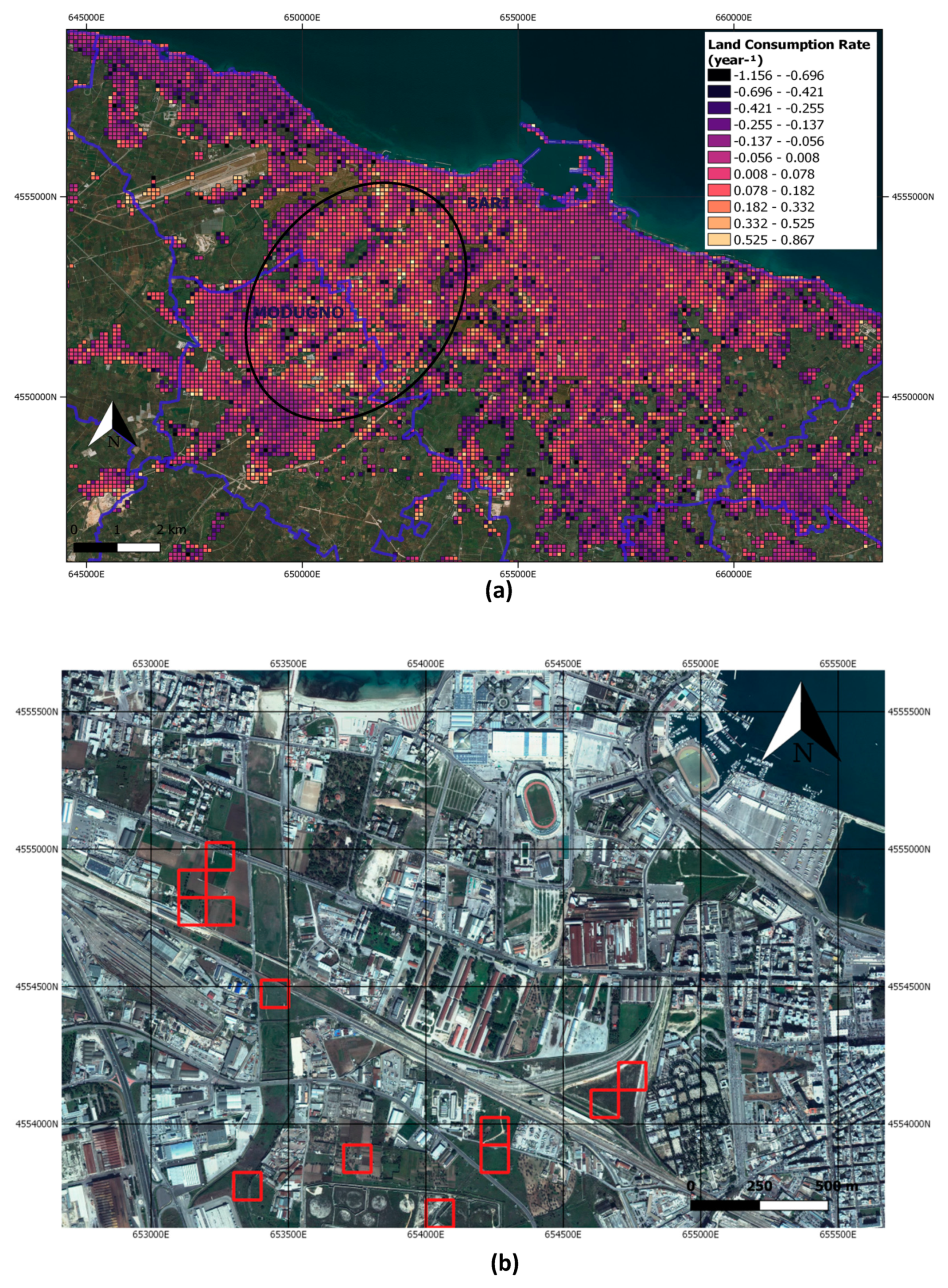
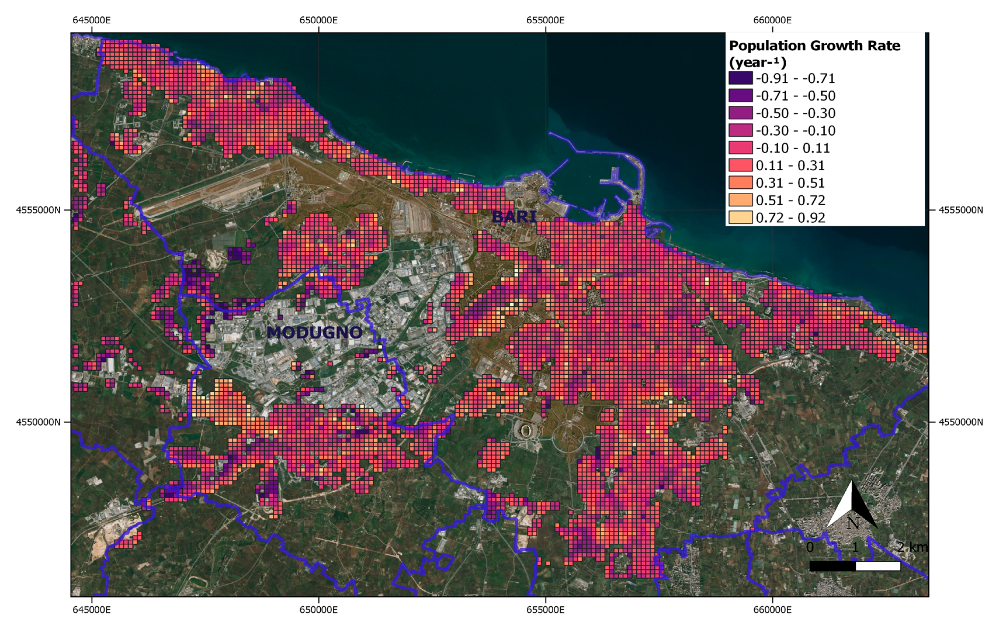
3.3. SDG 11.1.1. and SDG 11.3.1 Evaluation
4. Discussion
5. Conclusions
Author Contributions
Funding
Acknowledgments
Conflicts of Interest
References
- United Nations, Department of Economic and Social Affairs, Population Division. International Migration Report 2017: Highlights; UN: New York, NY, USA, 2017; Available online: https://www.un.org/en/development/desa/population/migration/publications/migrationreport/docs/MigrationReport2017_Highlights (accessed on 11 December 2018).
- United Nations. The Sustainable Development Goals Report 2017; UN: New York, NY, USA, 2017; Available online: https://unstats.un.org/sdgs/files/report/2017/thesustainabledevelopmentgoalsreport2017.pdf (accessed on 17 July 2017).
- United Nations, Department of Economic and Social Affairs, Population Division. International Migrant Stock 2019; UN: New York, NY, USA, 2019; Available online: https://www.un.org/en/development/desa/population/migration/publications/migrationreport/docs/MigrationStock2019_TenKeyFindings.pdf (accessed on 17 September 2019).
- Organization for Economic Cooperation and Development (OECD). International Migration Outlook 2019; OECD Publishing: Paris, France, 2019. [Google Scholar]
- SDG. Available online: https://www.un.org/sustainabledevelopment/sustainable-development-goals/ (accessed on 20 November 2015).
- Melchiorri, M.; Pesaresi, M.; Florczyk, A.J.; Corbane, C.; Kemper, T. Principles and Applications of the Global Human Settlement Layer as Baseline for the Land Use Efficiency Indicator—SDG 11.3.1. ISPRS Int. J. Geo-Inf. 2019, 8, 96. [Google Scholar] [CrossRef]
- Ehrlich, G.; Kemper, T.; Pesaresi, M.; Corbane, C. Built-up area and population density: Two Essential Societal Variables to address climate hazard impact. Environ. Sci. Policy 2018, 90, 73–82. [Google Scholar] [CrossRef]
- D4I. 2017. Available online: https://ec.europa.eu/knowledge4policy/migration-demography/data-integration-d4i_en. (accessed on 17 July 2017).
- Alessandrini, A.; Natale, F.; Sermi, F.; Vespe, M. High Resolution Map of Migrants in the EU; JRC Techical Report EUR 28770 EN; Publications Office of the European Union: Luxembourg, Belgium, 2017. [Google Scholar] [CrossRef]
- Batista e Silva, F.; Gallego, J.; Lavalle, C. A high-resolution population grid map for Europe. J. Maps 2013, 9, 16–28. [Google Scholar] [CrossRef]
- Langford, M. Refining methods for dasymetric mapping using satellite remote sensing. In Remotely Sensed Cities; Mesev, V., Ed.; Taylor & Francis: London, UK, 2003. [Google Scholar]
- Petrov, A. One hundred years of dasymetric mapping: Back to the origin. Cartogr. J. World Mapp. 2012, 49, 256–264. [Google Scholar] [CrossRef]
- GRASS. Available online: https://grass.osgeo.org/ (accessed on 20 September 2017).
- ESM. 2012. Available online: https://land.copernicus.eu/pan-european/GHSL/european-settlement-map (accessed on 15 March 2020).
- CLC. 2012. Available online: https://land.copernicus.eu/pan-european/corine-land-cover (accessed on 14 June 2019).
- Copernicus Land Monitoring Service. 2016. Available online: www.copernicus.eu (accessed on 9 July 2013).
- United Nations, General Assembly. Transforming Our World: The 2030 Agenda for Sustainable Development; UN: New York, NY, USA, 2015; Available online: https://sustainabledevelopment.un.org/post2015/transformingourworld (accessed on 25 September 2015).
- SDG 11.1.1. 2018. Available online: https://unstats.un.org/sdgs/metadata/files/Metadata-11-01-01.pdf (accessed on 14 February 2018).
- SDG 11.3.1. 2016. Available online: https://unstats.un.org/sdgs/metadata/files/Metadata-11-03-01.pdf (accessed on 19 July 2016).
- Figueiredo, L.; Honiden, T.; Schumann, A. Indicators for Resilient Cities. In OECD Regional Development Working Papers; OECD Publishing: Paris, France, 2018. [Google Scholar]
- Remote Sensing of Environment Journal–Special Issue “Earth Observation for the Sustainable Development Goals”. 2020. Available online: https://www.sciencedirect.com/journal/remote-sensing-of-environment/special-issue/10RFDS7BFNH (accessed on 17 January 2020).
- ANCI. Italian National Municipalities Association. Rapporto Cittalia 2013. Le Città Metropolitan; Digitalia Lab s.r.l.: Roma, Italy, 2013. [Google Scholar]
- ESA. 2014. Available online: https://sentinel.esa.int/web/sentinel/missions/sentinel-2 (accessed on 23 June 2015).
- Di Gregorio, A.; Jansen, L.J.M. Land Cover Classification System (LCCS): Classification Concepts and User Manual; Food and Agriculture Organization of the United Nations: Rome, Italy, 2005. [Google Scholar]
- Mountrakis, G.; Im, J.; Ogole, C. Support vector machines in remote sensing: A review. ISPRS J. Photogramm. Remote. Sens. 2011, 66, 247–259. [Google Scholar] [CrossRef]
- Open Street Map. Available online: https://www.openstreetmap.org (accessed on 15 March 2020).
- Adamo, M.; Tarantino, C.; Lucas, R.M.; Tomaselli, V.; Sigismondi, A.; Mairota, P.; Blonda, P. Combined use of Expert Knowledge and Earth Observation data for the Land Cover mapping of an Italian grassland area: An EODHAM system application. In Proceedings of the IEEE Geoscience and Remote Sensing Symposium, Milan, Italy, 26–25 July 2015; pp. 3065–3068. [Google Scholar]
- Congalton, R.G.; Kass, G. Assessing the Accuracy of Remotely Sensed Data: Principle and Practices, 2nd ed.; Taylor & Francis Group: Abingdon, UK, 2009. [Google Scholar]
- CLC. 2018. Available online: https://land.copernicus.eu/pan-european/corine-land-cover (accessed on 14 June 2019).
- Apulia Basin Authority. 2016. Available online: http://www.adb.puglia.it/public/news.php (accessed on 19 January 2016).
- DeLorenzo, N.; Dugger, A. Choroplet Map Esri; Census Bureau: Sutland, MD, USA, 2012. Available online: https://www.arcgis.com/apps/MapJournal/index.html?appid=75eff041036d40cf8e70df99641004ca (accessed on 15 March 2012).
- Mennis, J. Generating surface models of population using dasymetric mapping. Prof. Geogr. 2003, 55, 31–42. [Google Scholar]
- Pesaresi, M.; Huadong, G.; Blaes, X.; Ehrlich, D.; Ferri, S.; Gueguen, L.; Halkia, M.; Kauffmann, M.; Kemper, T.; Lu, L.; et al. A global human settlement layer from optical HR/VHR RS data: Concept and first results. IEEE J. Sel. Top. Appl. Earth Obs. Remote Sens. 2013, 6, 2102–2131. [Google Scholar] [CrossRef]
- Calka, B.; Bielecka, E. Reliability Analysis of LandScan Gridded Population Data. The Case Study of Poland. ISPRS Int. J. Geo-Inf. 2019, 8, 222. [Google Scholar] [CrossRef]
- INSPIRE, Data Specification on Buildings—Draft Technical Guidelines. Available online: https://inspire.ec.europa.eu/documents/Data_Specifications/INSPIRE_DataSpecification_BU_v3.0rc3.pdf (accessed on 4 February 2013).
- ESM Validation Report. 2016. Available online: https://land.copernicus.eu/user-corner/technical-library/the-european-settlement-map-validation-report/view (accessed on 9 July 2017).
- Lu, Z.; Im, J.; Quackenbush, L.J.; Halligan, K. Population estimation based on multi-sensor data fusion. Int. J. Remote. Sens. 2010, 31, 5587–5604. [Google Scholar] [CrossRef]
- Tier Classifications for Global SDG Indicators. 2019. Available online: https://unstats.un.org/sdgs/iaeg-sdgs/tier-classification/ (accessed on 15 October 2018).


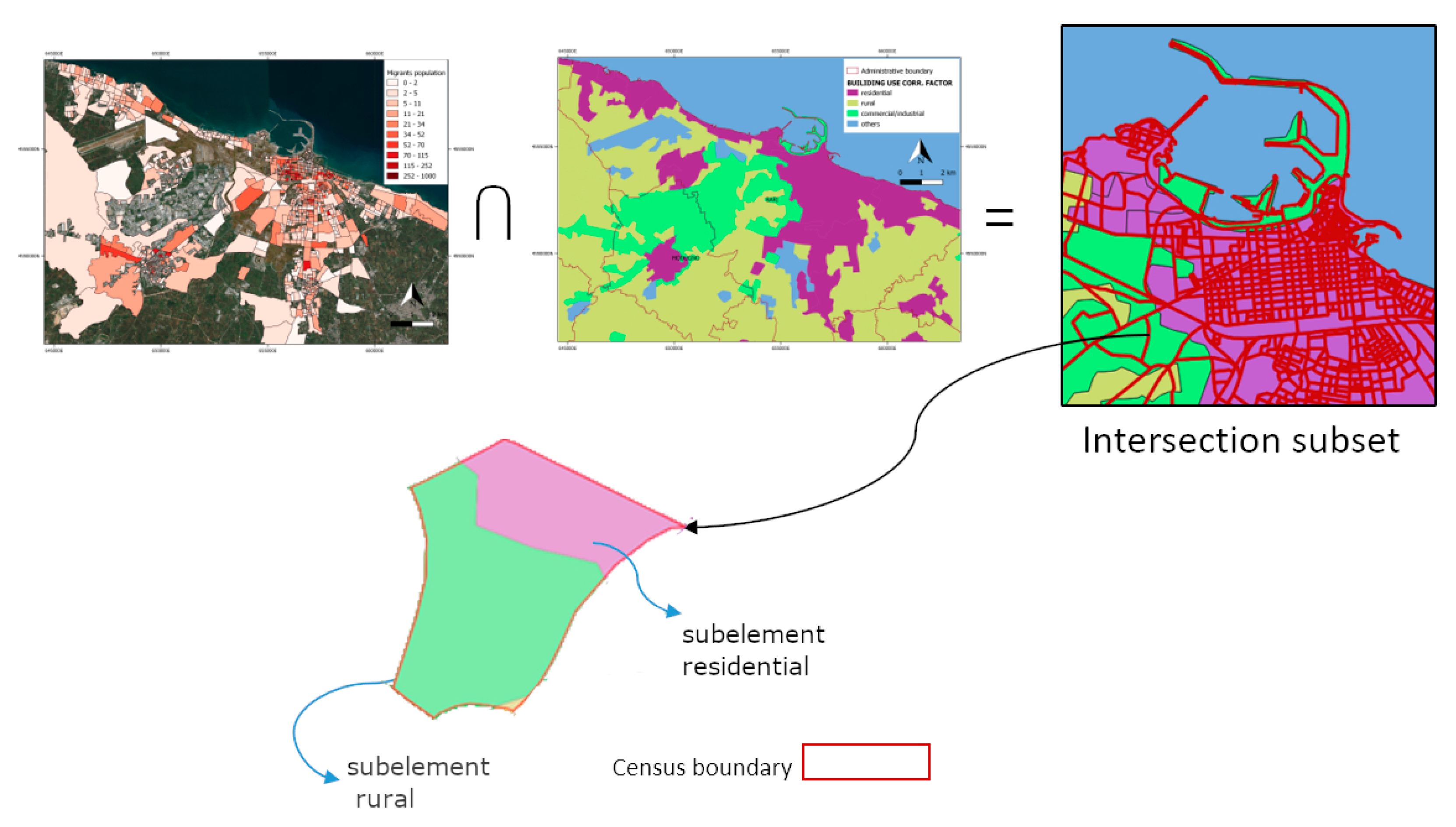
| Building use | CLC classes | Corrfactor |
|---|---|---|
| Residential | 1.1.1; 1.1.2 | 1 |
| Rural | 2.1.1; 2.1.2; 2.1.3; 2.2.1; 2.2.2; 2.2.3; 2.3.1; 2.4.1; 2.4.2; 2.4.3; 2.4.4 | 0.5 |
| Commercial/Industrial | 1.2.1, 1.2.3, 1.4.2 | 0.05 |
| Other | all remaining classes | 0.01 |
© 2020 by the authors. Licensee MDPI, Basel, Switzerland. This article is an open access article distributed under the terms and conditions of the Creative Commons Attribution (CC BY) license (http://creativecommons.org/licenses/by/4.0/).
Share and Cite
Aquilino, M.; Tarantino, C.; Adamo, M.; Barbanente, A.; Blonda, P. Earth Observation for the Implementation of Sustainable Development Goal 11 Indicators at Local Scale: Monitoring of the Migrant Population Distribution. Remote Sens. 2020, 12, 950. https://doi.org/10.3390/rs12060950
Aquilino M, Tarantino C, Adamo M, Barbanente A, Blonda P. Earth Observation for the Implementation of Sustainable Development Goal 11 Indicators at Local Scale: Monitoring of the Migrant Population Distribution. Remote Sensing. 2020; 12(6):950. https://doi.org/10.3390/rs12060950
Chicago/Turabian StyleAquilino, Mariella, Cristina Tarantino, Maria Adamo, Angela Barbanente, and Palma Blonda. 2020. "Earth Observation for the Implementation of Sustainable Development Goal 11 Indicators at Local Scale: Monitoring of the Migrant Population Distribution" Remote Sensing 12, no. 6: 950. https://doi.org/10.3390/rs12060950
APA StyleAquilino, M., Tarantino, C., Adamo, M., Barbanente, A., & Blonda, P. (2020). Earth Observation for the Implementation of Sustainable Development Goal 11 Indicators at Local Scale: Monitoring of the Migrant Population Distribution. Remote Sensing, 12(6), 950. https://doi.org/10.3390/rs12060950