Article

Nine-Year Systematic Evaluation of the GPM and TRMM Precipitation Products in the Shuaishui River Basin in East-Central China

1
Department of Environmental Science and Engineering, Fudan University, Shanghai 200433, China
2
Geography Section, School of Humanities, Universiti Sains Malaysia, Penang 11800, Malaysia
3
State Key Laboratory of Hydrology-Water Resources and Hydraulic Engineering, Nanjing Hydraulic Research Institute, Nanjing 210029, China
*
Author to whom correspondence should be addressed.
Remote Sens. 2020, 12(6), 1042; https://doi.org/10.3390/rs12061042
Submission received: 3 February 2020 / Revised: 18 March 2020 / Accepted: 21 March 2020 / Published: 24 March 2020
(This article belongs to the Special Issue Remote Sensing of Precipitation: Part II)

Abstract

:
Owing to their advantages of wide coverage and high spatiotemporal resolution, satellite precipitation products (SPPs) have been increasingly used as surrogates for traditional ground observations. In this study, we have evaluated the accuracy of the latest five GPM IMERG V6 and TRMM 3B42 V7 precipitation products across the monthly, daily, and hourly scale in the hilly Shuaishui River Basin in East-Central China. For evaluation, a total of four continuous and three categorical metrics have been calculated based on SPP estimates and historical rainfall records at 13 stations over a period of 9 years from 2009 to 2017. One-way analysis of variance (ANOVA) and multiple posterior comparison tests are used to assess the significance of the difference in SPP rainfall estimates. Our evaluation results have revealed a wide-ranging performance among the SPPs in estimating rainfall at different time scales. Firstly, two post-time SPPs (IMERG_F and 3B42) perform considerably better in estimating monthly rainfall. Secondly, with IMERG_F performing the best, the GPM products generally produce better daily rainfall estimates than the TRMM products. Thirdly, with their correlation coefficients all falling below 0.6, neither GPM nor TRMM products could estimate hourly rainfall satisfactorily. In addition, topography tends to impose similar impact on the performance of SPPs across different time scales, with more estimation deviations at high altitude. In general, the post-time IMERG_F product may be considered as a reliable data source of monthly or daily rainfall in the study region. Effective bias-correction algorithms incorporating ground rainfall observations, however, are needed to further improve the hourly rainfall estimates of the SPPs to ensure the validity of their usage in real-world applications.

Graphical Abstract

1. Introduction

Precipitation is an important component of the hydrological cycle [1,2]. Accurate and high-resolution precipitation data are crucial in different fields such as weather forecast, disaster preparation and prevention, and water resource management [3,4]. The quality and resolution of precipitation inputs can also significantly affect the performance of various hydrological, climatic, and atmospheric models [5].
However, obtaining suitable precipitation data could be challenging for researchers as well as practitioners. Availability of traditional ground observations has been limited because of the inadequate and uneven distribution of rain gauges, especially in developing countries, mountainous and remote areas, and over oceans [6]. On the other hand, although weather radar products can provide rainfall observations over a wide region [7], they are subjected to both random and systematic errors [8,9,10,11]. Random errors could arise from the sub-grid horizontal and vertical variability of rainfall and the noise of the radar hardware system, while systematic errors may originate from sources such as drifts in radar calibration constant, systematic variations in the reflectivity–rain-rate relationship, and strong gradients in the reflectivity profile [12]. The presence of complex topography may further amplify some of the error sources [13].
In recent years, with the rapid development of remote sensing techniques, satellite precipitation products (SPPs) have been increasingly applied in monitoring precipitation patterns [14,15,16]. Deriving precipitation products through satellite remote sensing has the advantages of wide coverage and high spatiotemporal resolution, which complement traditional ground gauge measurements. For example, the Tropical Rainfall Measuring Mission (TRMM) satellite launched in 1997 has been extensively used in hydrological modelling and climate change studies. Li et al. [17] found overall good linear relationships between TRMM and ground rainfall observations at both daily and monthly time steps in the Xinjiang catchment, China. Bharti and Singh [18] compared TRMM 3B42V7 with the gauge-based measurements at different altitudes in the northwest Himalayan region. They found that the satellite performed satisfactorily in the altitude range of 1000–2000 m, but poorly over higher-altitude regions at a daily time step.
In 2014, the National Aeronautics and Space Administration (NASA) of U.S. and JAXA (Japan Aerospace Exploration Agency) jointly developed a new generation of Global Precipitation Measurement (GPM) satellites. In addition to inheriting the advantages of the TRMM satellites in detecting precipitation in the tropics, GPM satellites provide global precipitation estimates for a wider quasi-global coverage (60° N–60° S) at a much higher spatiotemporal resolution (0.1° × 0.1° and 30-min interval). Much research has concluded that GPM products have improved in terms of both rainfall observation accuracy and hydrological simulation performance compared to TRMM products. For example, Tan et al. [19] and Sharifi et al. [20] compared the accuracy of rainfall observations between IMERG (integrated multi-satellite retrievals for GPM) and TRMM in Singapore and India, respectively. In both studies, all evaluation indices had indicated a better performance of IMERG than TRMM in providing monthly and daily rainfall data. In China, Tang et al. [21] analyzed the errors of IMERG and TRMM products in six sub-regions of Mainland China and found that IMERG had improved the accuracy of precipitation observations in the mid-high latitude as well as arid regions. In addition, they observed that IMERG could better reproduce the probability density function of rainfall, especially in the range of lower rainfall intensity.
In June 2019, the IMERG product was upgraded from Version 5 (V5) to Version 6 (V6) by reducing biases based on the new Global Precipitation Climatology Centre (GPCC) monthly precipitation records. Meanwhile, TRMM data before 2014 have also been reprocessed with the latest algorithm of the IMERG V6. Until now, few studies have been carried out to evaluate the performance of the latest IMERG and TRMM products.
Furthermore, the majority of previous research has evaluated SPP products at the monthly or daily scale, although both GPM and TRMM products contain hourly rainfall products. High quality hourly rainfall data have been found to be valuable to various hydrological applications around the world [22]. For example, Zhou and Wu [23] found that the precipitation intensity and distribution characteristics of typhoons in China could be better analyzed with hourly precipitation than daily observations at automatic weather stations. Yang et al. [24,25] found that the SWAT (Soil and Water Assessment Tool) model built on hourly rainfall could yield much better performance in simulating daily streamflow and monthly nutrient loads than the SWAT model built on daily rainfall in the Upper Huai River basin of China. Boithias et al. [26] found that the SWAT model built on hourly rainfall could better predict discharge over long periods of time than the MARINE model in the Mediterranean coastal Têt River basin (Southwestern France).
Compared to daily rainfall, hourly rainfall data are much more difficult to obtain because of several reasons. Firstly, much fewer gauges can or will record the amount of rainfall at an hourly or finer interval worldwide. Secondly, hourly rainfall data are generally not free to the public. Purchase of hourly rainfall data might be too expensive for researchers or practitioners in some regional studies. Finally, authorities in some regions may consider hourly rainfall records as sensitive data, thus denying their access to the public citing security reasons. In view of the limited access to hourly rainfall data globally, SPPs may provide a much-needed alternative for deriving such products. So far, few studies have been carried out to evaluate the capability of SPPs in providing hourly rainfall estimates.
To fill in the gaps, this study aims to evaluate the accuracy of the latest GPM and TRMM rainfall products across the monthly, daily, and hourly scales based on the ground rain gauge measurements between January 2009 and December 2017 in the Shuaishui River Basin (SRB) of eastern Central China. The Shuaishui River is the headwater tributary to the Qiantangjiang River, the main river flowing across the Zhejiang Province of China. With water quality inferior to the Class III standard at 50.5% of its total river length, the Qiantangjiang River Basin is faced with severe water security concerns [27,28]. As the critical ecological barrier to the Qiantangjiang River, the hydrological conditions of the SRB has direct impact on the downstream ecological environment.
Essentially a hilly watershed, SRB is characterized with complex terrains and obvious vertical height difference. Precipitation in the basin is abundant, but also highly seasonal. Steep slopes combined with ample rainfall in summer have aggravated the risk of natural disasters such as floods and mudslides [29]. The flood in June 2016 in the SRB, for instance, has affected 58,000 people with a direct economic loss of 168 million RMB. SRB, therefore, presents an ideal referencing region for evaluating the suitability of using SPPs in the sub-tropical hilly regions with large inter-annual and intra-annual rainfall variabilities.

2. Study Area

Approximately 159 km in length, the Shuaishui River originates from the Hutou mountain ranges and flows across the Xiuning County before pouring into the Xinanjiang River at the Tunxi district of Huangshan City. The SRB (117°39′–119°26′ E and 29°24′–31°1′ N) has a total area of 1522 km2 (Figure 1). Dominated by a hilly terrain, more than 70% of the basin is at an altitude of above 500 m. Land use and land cover in the basin is mainly forestland and cultivated land, which respectively accounts for 78.9% and 14.6% of the total coverage.
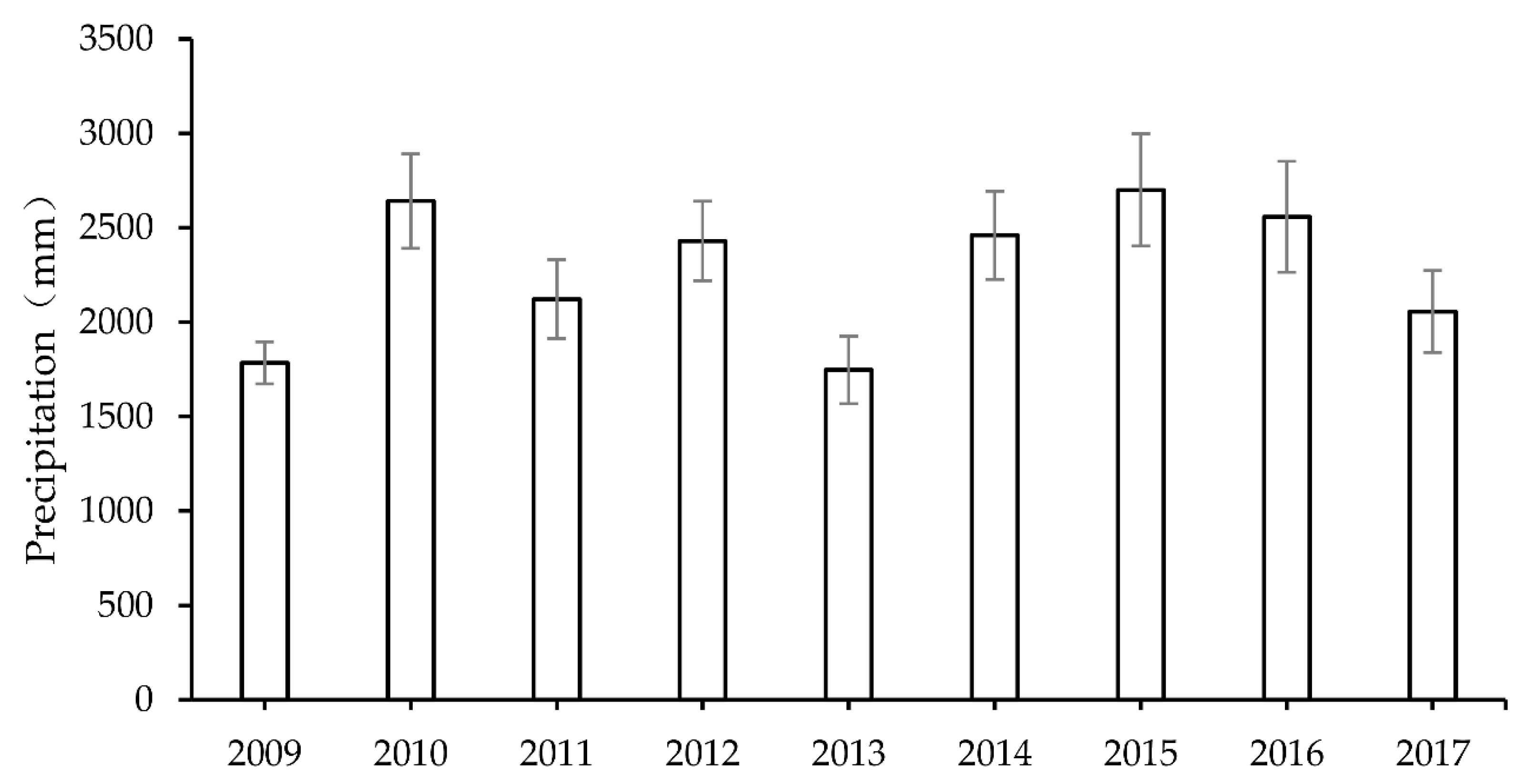
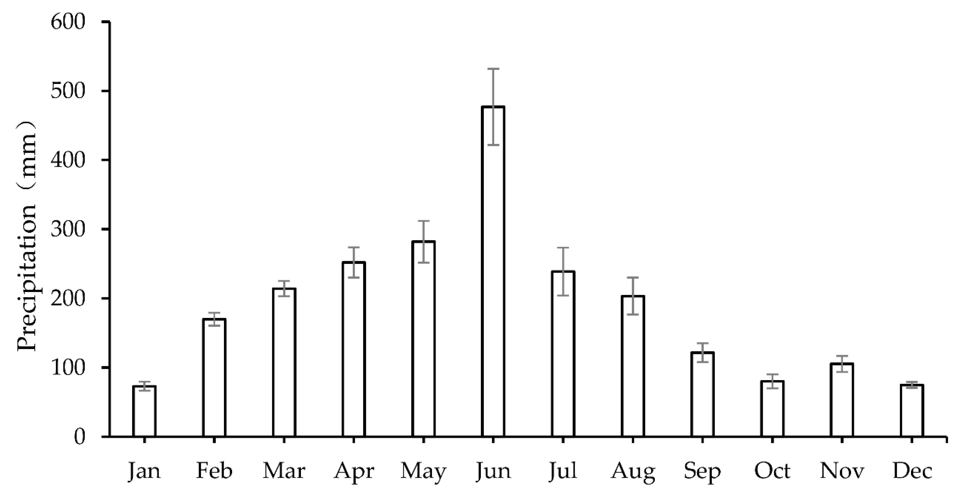
Located in the subtropical monsoon climate zone, rainfall in the SRB is usually abundant. Between 2009 and 2017, mean annual rainfall observed by rain gauges in the basin ranges from 1747 mm in 2013 to 2700 mm in 2015 with an overall average of 2278 mm (Figure A1). Within each year, mean monthly rainfall usually increases steadily from January to May and peaks in June. Precipitation in June alone could account for more than one-fifth of annual total rainfall. After June, monthly rainfall falls sharply and exhibits an overall decreasing trend till the end of the year (Figure A2).

3. Materials and Methods

3.1. Satellite Precipitation Products

The TRMM satellite was launched in 1997 through a joint space mission between the NASA of U.S. and the National Space Development Agency of Japan [30]. TRMM carries five instruments, including a suite of three rainfall sensors (Precipitation Radar (PR), TRMM Microwave Imager (TMI), Visible and Infrared Sensor (VIRS)) and two related instruments (Lightening Imaging Sensor (LIS) and Clouds and the Earth’s Radiant Energy System (CERES)). The TRMM Multi-satellite Precipitation Analysis (TMPA) products combine infrared (IR) data from geostationary satellites, such as GOES-W, GOES-E, GMS, Meteosat-5, Meteosat-7, and NOAA-12, with microwave (MW) data from multiple satellites including TMI/TRMM (TRMM Microwave Imager), SSMI/DMSP (Special Sensor Microwave Imager/Defense Meteorological Satellite Program), AMSU/NOAA (Advanced Microwave Sounding Unit/National Oceanic and Atmospheric Administration), and AMSR-E (Advanced Microwave Scanning Radiometer-EOS) [31]. The TMPA products are produced in the following four stages. First, the MW precipitation estimates are calibrated and combined using algorithms such as sensor-specific versions of the Goddard Profiling Algorithm (GPROF). Secondly, IR precipitation estimates are created using the calibrated MW precipitation. Thirdly, the MW and IR precipitation estimates are combined. Finally, rain gauge data are incorporated. Detailed descriptions of the algorithms and steps for producing the TMPA products could be found in Huffman et al. (2007) [32] and Huffman et al. (2018) [33].
In May 2012, the TMPA was upgraded from version 6 (V6) to version 7 (V7) by implementing the latest version of re-calibration algorithm and using the new GPCC monthly precipitation products for bias correction. The TMPA 3B42 consists of two products: the near-real-time product (3B42RT) and the post-processed product (3B42). The 3B42RT product, which is released approximately 9 h after real-time, spans the latitude belt from 50° N to 50° S. In contrast, with a more extensive coverage from 60° N to 60° S, the 3B42 product is released 10–15 days after each month when the bias correction has been made based on ground gauge records.
As a global successor of TRMM, the GPM project is launched in 2014 to provide global precipitation observations. The GPM satellite is equipped with an advanced Dual-frequency Precipitation Radar (DRP) that observes the internal structure of storms within and under the clouds, and a GPM Microwave Imager (GMI) that measures the type, size, and intensity of precipitation. The DPR is more sensitive than its TRMM predecessor especially in the measurement of light rainfall and snowfall in high latitude regions.
In March 2014, NASA released its first GPM-era global precipitation product–IMERG (Integrated Multi-satellites Retrievals for GPM). The IMERG algorithm is designed to inter-calibrate, interpolate, and merge all available satellite MW precipitation estimates, MW-calibrated IR satellite estimates, gauge measurements, and other potential precipitation estimates at fine spatial and temporal resolution worldwide. Its inter-calibration of available MW data is similar to TMPA, but further interpolated and re-calibrated by the Climate Prediction Center (CPC) morphing Kalman Filter technique and the Precipitation Estimation from Remotely Sensed Information using Artificial Neural Networks—Cloud Classification System (PERSIANN-CCS) [34,35].
IMERG includes three products with different latencies: the near-real-time ‘Early’ (near real-time with a latency of 6 h) run (IMERG-E), the near-real-time ‘Late’ (reprocessed near real-time with a latency of 18 h) run (IMERG-L), and the post-real-time ‘Final’ (gauge-adjusted with a latency of four months) run (IMERG-F). The algorithm for the IMERG was upgraded from Version 5 (V5) to Version 6 (V6) to reduce bias and improve consistency among different IMERG runs in June 2019. For example, the ‘displacement vectors’ in V6 are computed using the Modern Era Retrospective Reanalysis 2 (MERRA-2) and Goddard Earth Observing System (GEOS) model Forward Processing (FP) data instead of the previously used infrared data, which helps ensure consistency in the vectors between the Final Run and the Early and Late Runs.
In this study, we aim to evaluate the performance of a total of five SPPs in the SRB, including the Early, Late, and Final runs of the IMERG V6 products (0.1° × 0.1° and 30-min interval), and the near-real-time and post-processed runs of the TMPA V7 products (0.25° × 0.25° and 3-hour interval). The SPPs datasets are all downloaded from the NASA website (https://disc.gsfc.nasa.gov/). After being downloaded, the SPPs datasets are adjusted to the local time, which is eight hours ahead of Coordinated Universal Time (UTC). Since the IMERG V6 and TMPA V7 products respectively contain 30-min and 3-h rainfall estimates, they need to be processed before being evaluated at different temporal scales. At the daily and monthly scale, both IMERG and TMPA data are directly aggregated to the corresponding levels for comparison with ground measurements. For evaluation at the hourly scale, the TMPA hourly rainfall estimates are obtained by assuming a constant rainfall intensity over the 3-hour period.

3.2. Ground Rainfall Measurements

Hourly and daily precipitation records from 2009 to 2017 at a total of 13 rainfall stations in the SRB (Figure 1) are obtained from the hydrological yearbook series published by Ministry of Water Resources of China. The rain gauges used at the rainfall stations are tipping buckets. All of the rainfall data have gone through strict quality control following the relevant China’s industry standards such as QX/T 118-2010 (quality control of surface meteorological observation data) before being published. There are no rainfall data missing at the 13 stations. In the SRB, daily rainfall has been recorded throughout the year, while hourly rainfall only documented for the relatively wet period from April to October. Correspondingly, the monthly and daily estimates of the SPPs are evaluated throughout the year, while their hourly estimates are only assessed within the seven months.

3.3. Evaluation Metrics

A total of four continuous metrics are used to evaluate the quality of satellite precipitation products in the SRB. Correlation coefficient (CC) is used to quantify the linear correlation between satellite precipitation estimates and ground measurements; it varies between −1 and 1, with a value close to 0 indicating little correlation. Root-mean-square error (RMSE) quantifies the degree of dispersion between satellite precipitation and measured precipitation, which can reflect the overall error level and accuracy of SPPs [36]; mean absolute difference (MAD) evaluates the magnitude of the average difference between satellite precipitation and measured precipitation. Smaller values of RMSE and MAD indicate a better performance of the SPPs. Relative bias (RB) measures the systematic bias of satellite precipitation compared with gauge observations. A positive and negative RB indicates overestimation and underestimation, respectively. As a rule of thumb, SPPs can be considered as reliable when RB falls between −10% and 10% and CC exceeds 0.7 [37].
The four continuous metrics are calculated as [38,39,40]
C C = i = 1 n ( X i o X ¯ o ) ( X i s X ¯ s ) i = 1 n ( X i o X ¯ o   ) 2 i = 1 n ( X i s X ¯ s ) 2
R B = i = 1 n ( X i s X i o ) i = 1 n X i o × 100 %
R M S E = i = 1 n ( X i s X i o ) 2 n
M A D = i = 1 n | X i o X i s | n
where n is the number of the simulated and observed data pairs; X i s and X i o denote the ith simulated and observed amount, respectively; X ¯ s and X ¯ o are the mean of the simulated and observed data, respectively.
Besides the continuous metrics, three categorical evaluation metrics are used to evaluate the precipitation detection capability of the SPPs, which include probability of detection (POD), false alarm rate (FAR), and critical success index (CSI). POD represents the ratio of correctly detected precipitation occurrences by the SPPs to the total number of actual precipitation occurrences. With an optimal value of 1, a higher POD indicates that the SPP is more capable of detecting the actual precipitation occurrences. FAR calculates the ratio of falsely detected precipitation occurrences to the total number of detected precipitation occurrences. With an optimal value of 0, a lower FAR indicates that the SPP is less likely to yield false precipitation occurrences. CSI incorporates both missed events and false detections in its calculation [41]. With an optimal value of 1, a higher CSI indicates a better performance of the SPP with more correct detections as well as fewer false alarms of precipitation occurrences. Based on the number of hits (H), false alarms (F), and misses (M) (Table 1), the three categorical metrics are calculated as
P O D = H H + M
F A R = F H + F ,
C S I = H H + M + F
where S represents rain gauge observation; P represents satellite rainfall estimate; H (hits) represents the number of cases when both the rain gauge and the satellite determine the rainfall to equal or exceed the threshold; F (false alarms) represents the number of cases when the satellite determines the rainfall to equal or exceed the threshold but not the rain gauge; M (misses) represents the number of cases when the rain gauge determines the rainfall to equal or exceed the threshold but not the satellite; and Z (correct negatives) represents the number of cases when both the rain gauge and the satellite determine the rainfall to fall below the threshold.

3.4. Analysis of Variance (ANOVA)

To evaluate the rainfall estimation performance of the five satellite precipitation products, four continuous metrics (CC, RB, RMSE, and MAD) are respectively calculated at each of the 13 rainfall stations across the monthly, daily, and hourly scales. Previous studies have mostly used the mean values of the metrics over all rainfall stations to compare the rainfall estimation performance among the SPPs. This simple averaging approach, however, does not account for the variability in the metrics among the rainfall stations. Furthermore, it is incapable of determining the significance of the difference between the SPPs.
In view of the deficiency, we adopt the one-way analysis of variance (ANOVA) to statistically evaluate the difference in metrics between the SPPs. In the ANOVA, satellite precipitation product type is used to designate the five groups of metrics for comparison. If the ANOVA determines there is some significant difference in the mean metrics among the SPPs, multiple commonly used posterior comparison tests—including the Bonferroni, Sidak, Tukey, and Scheffe tests built in the Origin 2018 Statistical Package—are further used to identify the pairs of SPPs whose mean metrics are indeed statistically different.

4. Results and Discussions

4.1. Evaluation at the Monthly Scale

4.1.1. Temporal Analysis

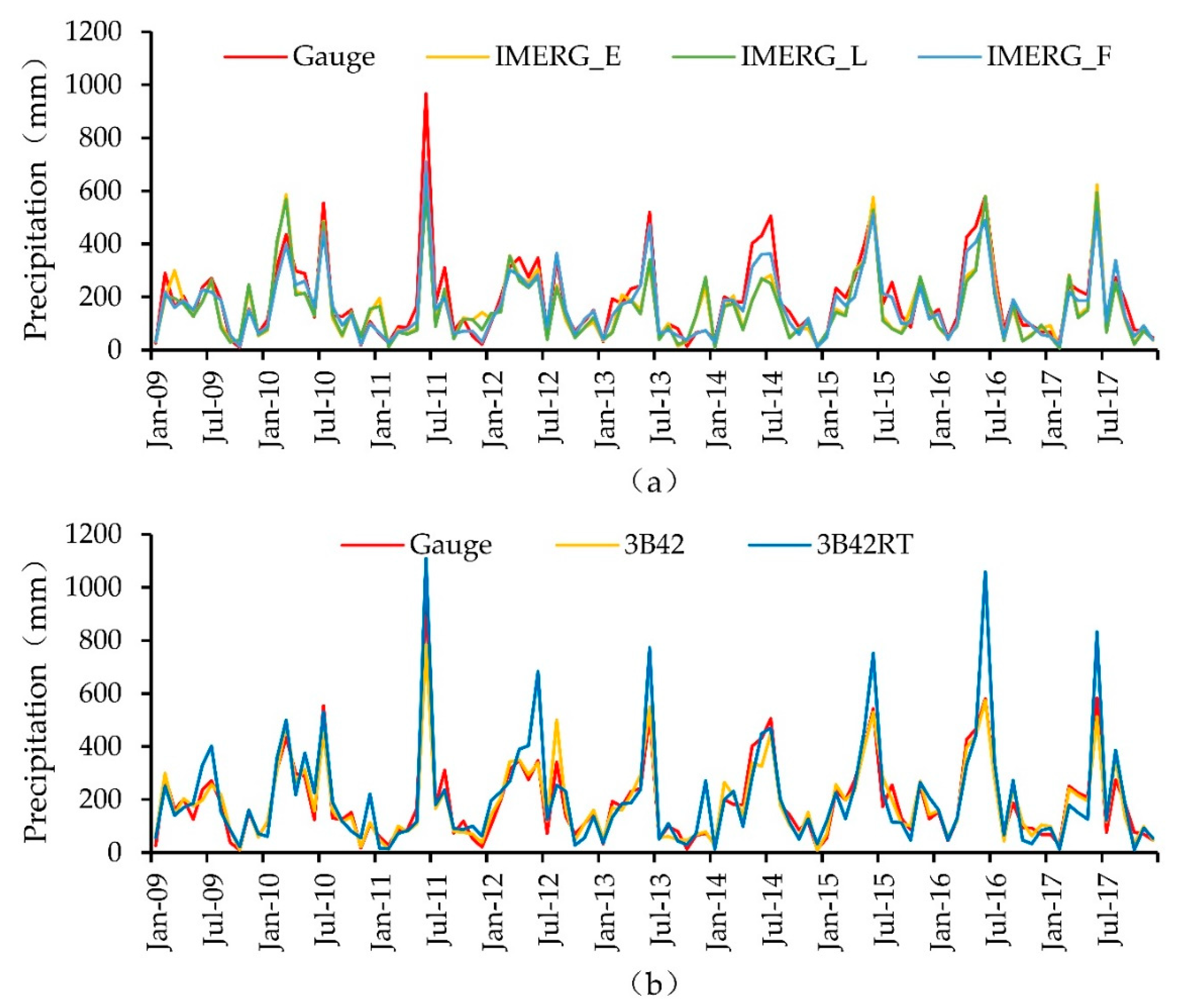
Figure 2 compares the mean of the observed monthly precipitation in the SRB with that of the five SPPs from January 2009 to December 2017. Figure A3 compares the scatterplots between observed and estimated monthly rainfall among the SPPs. In general, all five SPPs are capable of capturing the overall trend of monthly precipitation variations. The annual CCs of the five SPPs are all above 0.85, while those of IMERG_F and 3B42 even exceed 0.95. The IMERG products all exhibit a tendency of underestimating rainfall, especially in wet months. In particular, for June, 2011 whose monthly rainfall reached as high as 1109 mm, IMERG_E, IMERG_L, and IMERG_F give a low estimate of 608, 608, and 710 mm, respectively.
Table 2 compares the mean values of the four continuous evaluation metrics over the 13 rainfall stations among the five SPPs both annually and seasonally. With the highest RMSE of 101.42 mm and MAD of 65.72 mm, the 3B42RT product deviates the most from historical rainfall observations annually. A closer examination of the seasonal changes in RMSE and MAD, however, have shown that its considerably larger deviation in summer is the main cause. In the three seasons other than summer, 3B42RT actually deviates less than the two near-real-time IMERG products (Table 2).
Annually, the three IMERG products tend to underestimate monthly precipitation, while the two TMPA products behave the opposite. Seasonally, IMERG_F tend to underestimate monthly precipitation throughout the year, while the other two IMERG products act the same except that they tend to slightly overestimate in winter. In contrast, the RB of 3B42 remains close to zero all over the year except it approaches 10% in winter. Meanwhile, the RB of 3B42RT fluctuates much more ranging from -4.9% in spring to 25.8% in summer (Table 2). In terms of the other three continuous metrics, the five SPPs have exhibited somewhat similar seasonal patterns of change. For example, the CCs of the SPPs all reach or approach their peak values in summer, while decreasing to the bottom in fall. Meanwhile, both the RMSEs and MADs of the SPPs all rise to the top in summer, drop to medium in spring, and down to the lowest in fall and winter (Table 2). The seasonal changes in RMSEs and MADs correspond closely to the changes in the magnitude of seasonal rainfall.
Except for RB, the two post-time products (IMERG_F and 3B42) perform significantly better than the rest real-time or near real-time products both annually and seasonally, with a noticeably higher value of CC (e.g., 0.97 and 0.95 annually) as well as considerably lower values of RMSE (e.g., 53.82 and 54.13 mm annually), and MAD (e.g., 35.79 and 37.07 mm annually) (Table 2). The findings of the overall better performance of the two post-time SPPs products compared to the real-time or near real-time products at the monthly time scale are not surprising, since both are generated after the adjustment of real-time products based on monthly measurements of ground rain gauges [42], although which may not include the 13 rain gauges covered in our study. With their annual CC and RB values exceeding the good performance thresholds, both IMERG_F and 3B42 can be regarded as reliable sources of monthly precipitation in the SRB. Similar to our study, previous studies have also observed satisfactory performance of IMERG_F and 3B42 in monthly rainfall estimation [43,44].

4.1.2. Spatial Variation

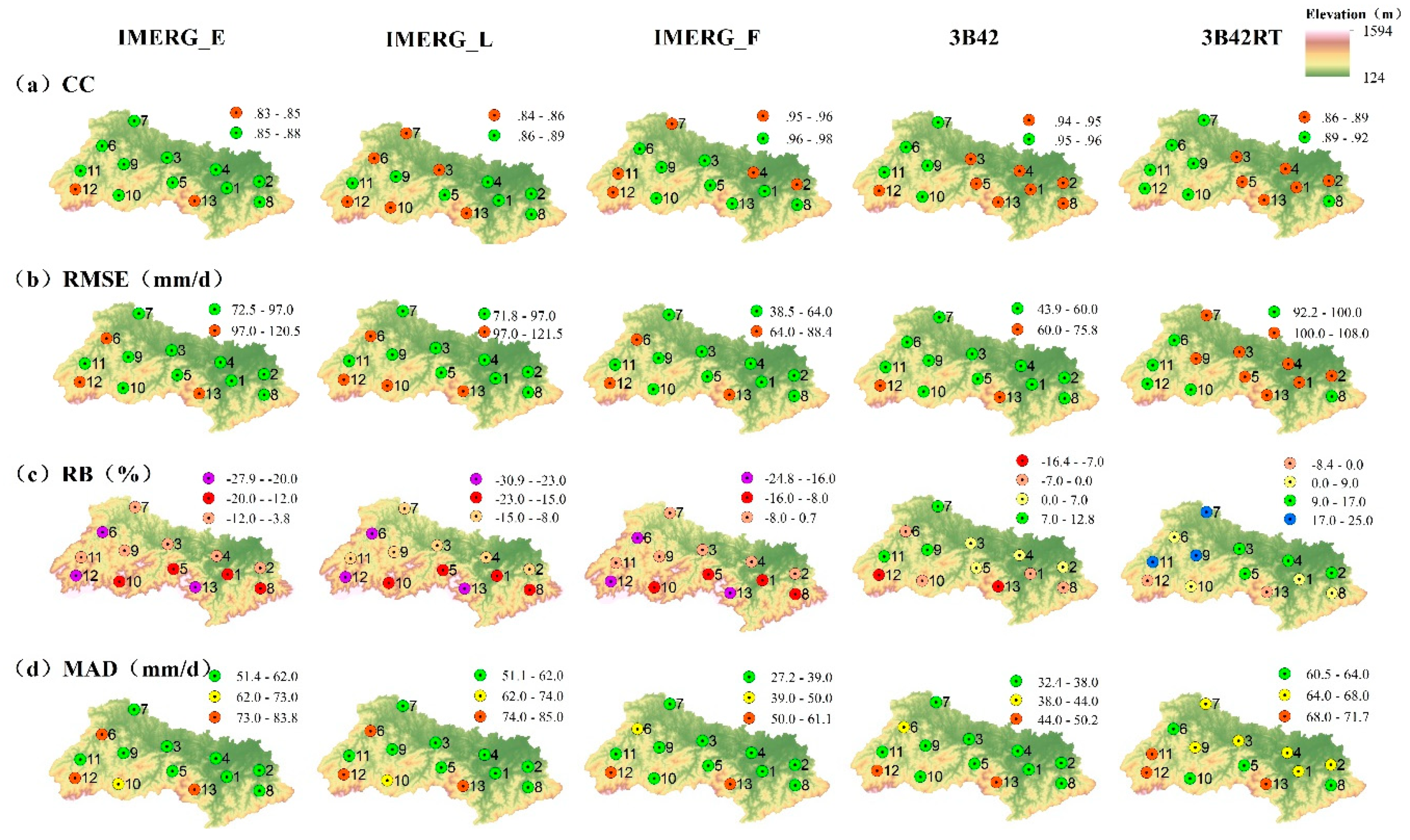
Figure 3 compares the spatial distribution of the four annual continuous evaluation metrics among the SPPs at the monthly scale. The spatial distributions of the CCs varies considerably among the IMERG products, while staying similar between the TMPA products. Topography does not seem to be a significant influencing factor of the CCs, although some stations at higher altitude (station 12 and 13) do have lower CCs in all five SPPs. In terms of RMSEs and MADs; however, topography plays a more eminent role. For all five SPPs, both metrics tend to get larger at higher altitude. In particular, RMSEs and MADs of three stations at high altitude (station 10, 12, and 13) consistently surpass those of the rest stations. In addition, the RBs exhibit a similar spatial pattern among the IMERG products. They all tend to underestimate monthly rainfall more severely at high altitude (e.g., stations 12 and 13). However, for the TMPA products, no clear pattern in the spatial distribution of RB could be observed.
Similar to our study, Milewski et al. [45] also found that elevation was a key factor affecting the accuracy of the TMPA products in Northern Morocco. The CCs of all four TMPA products at the low elevation class (0–500 m) consistently surpassed those at the medium (500–1000 m) and high (>1000 m) elevation classes. Contrary to the CCs, the normalized RMSEs at the low elevation class were consistently smaller.

4.2. Evaluation at the Daily Scale

Figure A4 compares the scatterplots between observed and estimated daily rainfall among the SPPs. Daily rainfall estimates by the IMERG_F cluster the closest around the 1:1 line, while 3B42RT estimates deviating the largest with a strong tendency of overestimation. For the daily scale assessment of SPPs, four continuous (CC, RMSE, RB, and MAD) and three categorical (POD, CSI, FAR) evaluation metrics are calculated using daily rainfall records at the 13 rainfall stations and the corresponding SPP estimates from 1 January 2009 to 31 December 2017.

4.2.1. Continuous Evaluation Metrics

(1) Temporal Variation

Table 3 compares the mean values of the continuous evaluation metrics among the SPPs at the daily scale. Annually, all four continuous evaluation metrics except RB have indicated a relatively better performance by the IMERG products in estimating daily rainfall. For example, the annual RMSEs of the IMERG products range from 9.66 mm/d (IMERG_F) to 11.30 mm/d (IMERG_E), while those of the TMPA products both exceed 11.50 mm/d. Seasonally, however, while IMERG_F generally remains the best product for estimating daily rainfall, the other two near-real-time IMERG products tend to perform better than the TMPA products in spring and summer, but often worse in fall and winter (except for RB).
Within each SPP family, the order of the daily rainfall estimation accuracy is largely consistent, i.e., IMERG_F > IMERG_L > IMERG_E (except for RB) and 3B42 > 3B42RT. Moreover, except for RB, the five SPPs have exhibited rather similar seasonal patterns of change in their daily metrics. For example, the CCs of the five SPPs all peak in summer and fall to the bottom in fall. The RMSEs and MADs of the SPPs all tend to peak in summer, decline in spring, and down to the lowest in fall and winter. Throughout the year, the Shuaishui River Basin is affected by different climatic systems. Mainly under the influence of the high-altitude trough, precipitation in fall and winter is mostly brought by stratiform clouds, which tends to be stable and therefore easier to measure. In spring and summer, however, the convective component in the precipitation system increases due to the Meiyu front and shear line system. Both thermal convection precipitation under the control of the Western Pacific Subtropical High (WPSH) and rainstorms caused by the typhoon system increase the difficulty of obtaining accurate measurement of rainfall because of their characteristics of short duration and high spatial heterogeneity. The differences in climatic systems have led to different seasonal rainfall characteristics, with more rainy days and higher rainfall intensity in spring and summer than in fall and winter. Between 2009 and 2017, there have been 529 and 589 rainy days in spring and summer, compared to 425 and 452 days in fall and winter. Days with precipitation < 1 mm account for 44.2% and 41.8% in fall and winter, compared to 30.6% and 26.7% in spring and summer. Meanwhile, days with precipitation > 50 mm account for 4.9% and 8.3% in spring and summer, compared to around 1.5% in fall and winter. The CCs’ peaking in summer could be attributed to the season’s large variability in daily rainfall, whose general pattern of change is relatively well captured by the SPPs. However, because there are more days with heavy precipitation in summer, the absolute errors of SPP estimates remain the largest in the season. Similarly, the lowest RMSEs and MADs in fall and winter are probably owing to their dominance of days with lower precipitation.
Similar to our findings, Su et al. [46] concluded that the post-time IMERG-F product, with a CC of 0.79, RMSE of 6.31 mm/d, and RB of 9.04%, was the best IMERG product for estimating daily rainfall in the Upper Huai River Basin of China. Meanwhile, Anjum et al. [43] found the post-time 3B42 V7 product, with a CC of 0.70 and RB of 14.77%, performed better than the real time 3B42RT product for estimating daily rainfall in Pakistan.
Compared to those at the monthly scale, the CCs of all five SPPs have decreased considerably at the daily scale. For instance, the annual CC of IMERG_F drops from 0.97 at the monthly scale to 0.81, while the annual CCs of the other SPPs all drop further to around 0.75. In contrast to the CCs, the RBs of the SPPs at the daily scale are more similar to those at the monthly scale in terms of both their signs and magnitude. Annually, all three IMERG products tend to underestimate daily precipitation with the lowest RB of −9.99%, while both TMPA products tend to overestimate with the lowest RB of 1.21%. Seasonally, the IMERG family products tend to underestimate daily rainfall in all four seasons except the two near-real-time products in winter. In contrast, 3B42RT exhibits a strong tendency of overestimation in summer and winter, while 3B42 only in winter.

(2) Statistical Performance Comparison among the SPPs

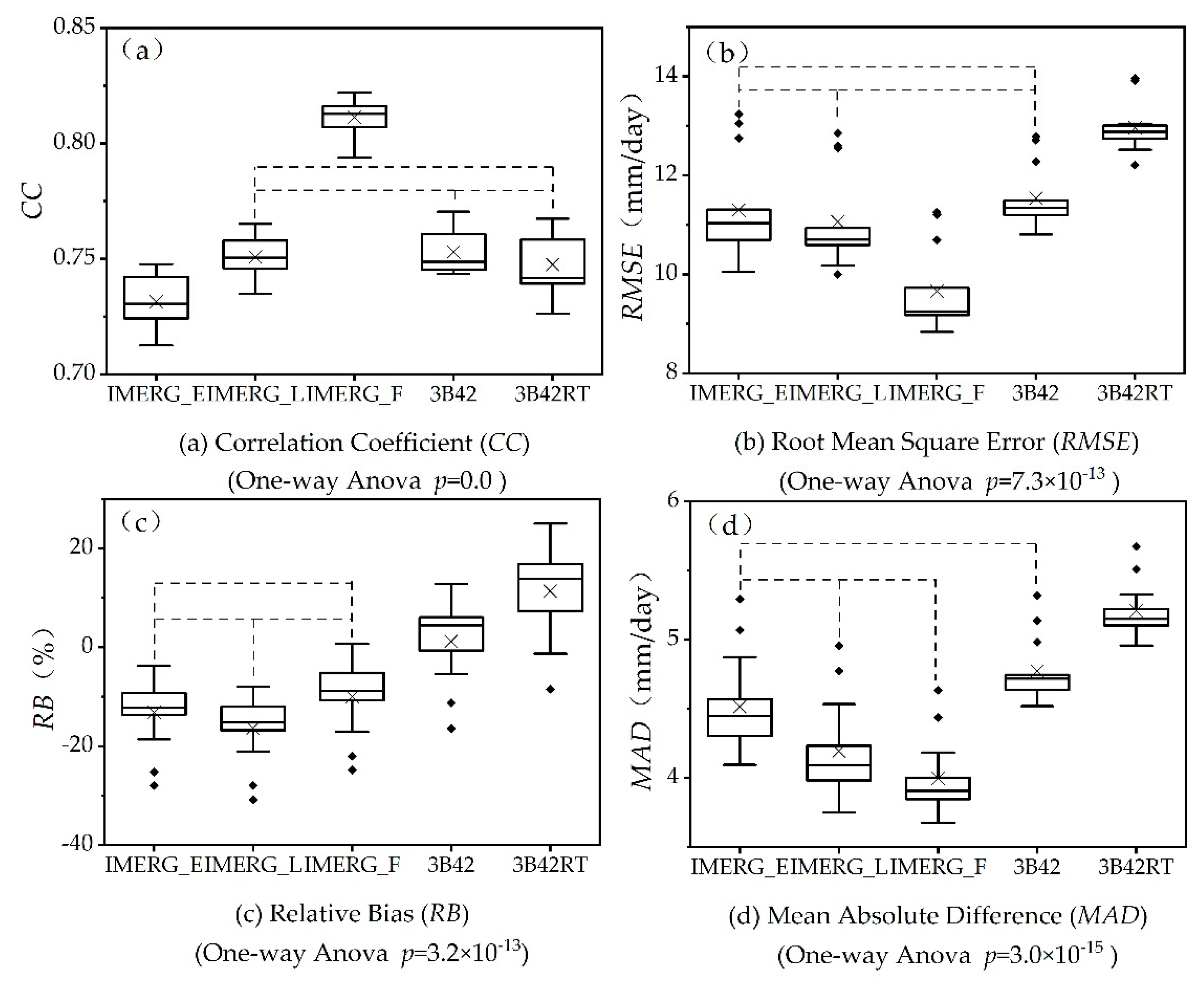
Figure 4 compares the boxplots of the four annual continuous evaluation metrics among the five SPPs. For example, Figure 4a contains five boxplots, which respectively depict the distribution of annual CCs of the five SPPs across the 13 rainfall stations. At the daily scale, the annual CCs of the IMERG_F range from 0.79 to 0.82 among the 13 rainfall stations, compared to 0.71–0.75 for IMERG_E, 0.73–0.77 for IMERG_L and 3B42RT, and 0.74–0.77 for 3B42.
One-way ANOVA could be used to assess whether the mean values of the four continuous metrics are significantly different among the five SPPs. One critical pre-condition of performing ANOVA is to ensure the homogeneity of variance among the compared groups. In this study, we use the Levene’s Test to compare the variance of the metrics among the five SPPs, which confirm that all four metrics could meet the requirement of homogeneity of variance. The subsequent one-way ANOVA has concluded that the mean values of all four metrics are significantly different among the SPPs at the significance level (α) of 0.05 (Figure 4).
In view of the significant ANOVA results, multiple posterior comparison tests—including the Bonferroni, Sidak, Tukey, and Scheffe tests—are further conducted to identify the pairs of SPPs whose mean metrics are truly significantly different. In Figure 4, two SPPs are connected with a black dotted line if posterior comparison tests have concluded a non-significant difference between their means at the α level of 0.05. As shown in the figure, the mean values of CC are significantly different between all pairs of SPPs except between IMERG_L and the two TMPA products as well as between the TMPA products themselves; the mean values of RMSE are all significantly different except between 3B42 and the two near real-time IMERG products as well as between the two near real-time IMERG products themselves; the mean values of RB are all significantly different except between the three pairs of IMERG products; the mean values of MAD are all significantly different except between IMERG_L and the other two IMERG products as well as between IMERG_E and 3B42. It is worth noting that the posterior comparison tests have shown that IMERG_F is the single IMERG product that is significantly different from the TMPA products in terms of all four metrics.

(3) Spatial Variation

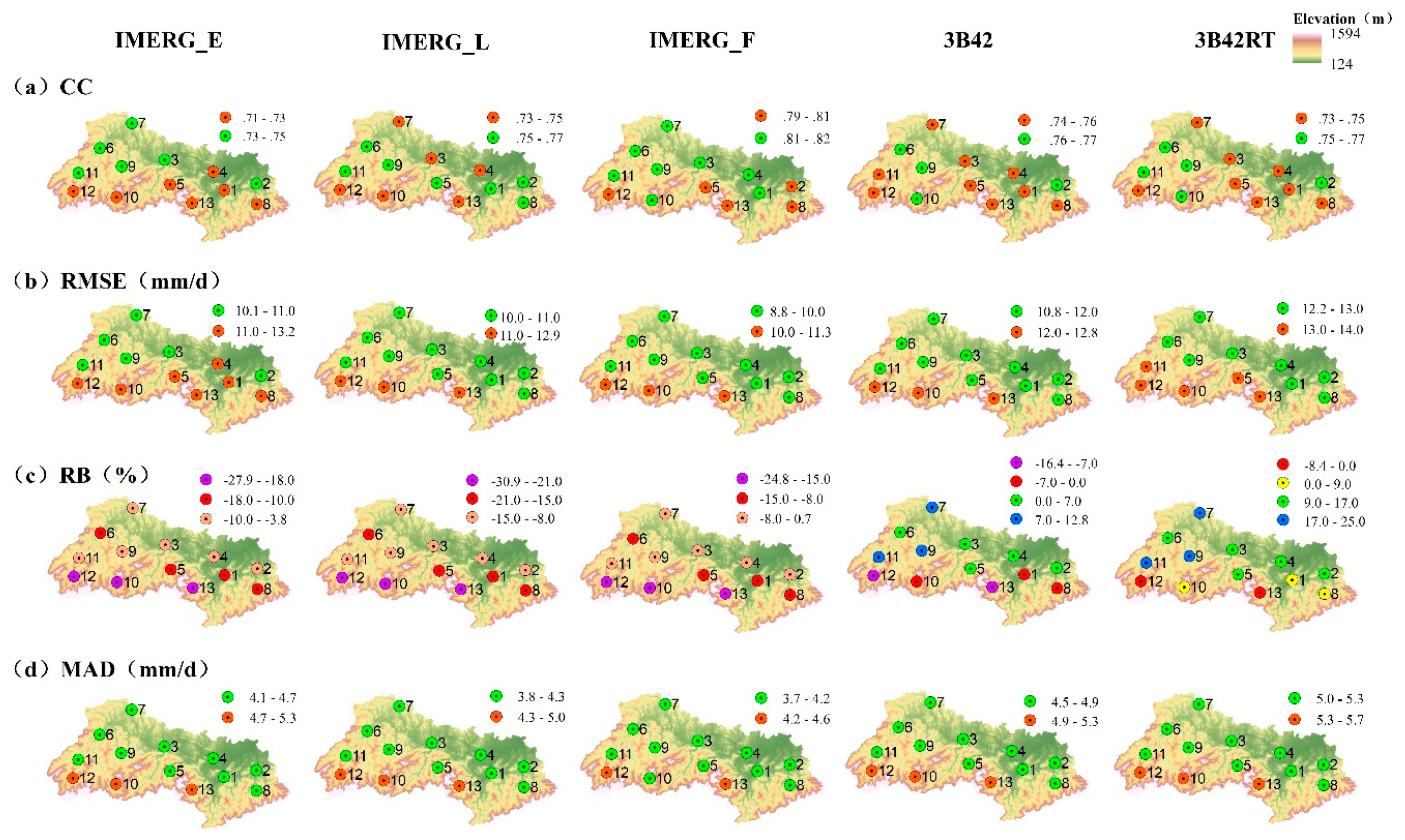
Figure 5 compares the spatial distribution of the four annual continuous evaluation metrics at the daily scale among the SPPs. The spatial distribution of the CCs varies considerably among the IMERG products, while staying similar between the TMPA products. Topography does not seem to be a significant influencing factor of the CCs, although all five SPPs have lower CCs at some stations of higher altitude (station 12 and 13). In terms of RMSEs and MADs, however, topography plays a more eminent role. For all five SPPs, both metrics tend to get larger at higher altitude. In particular, RMSEs and MADs of three stations at high altitude (stations 10, 12, and 13) consistently surpass those of the rest stations. In addition, topography seems to affect the RBs of the IMERG products considerably, which tend to underestimate daily rainfall more seriously at high altitude. The impact of topography on the RBs of the TMPA products, however, is rather mixed. The absolute RB of the 3B42RT product is actually smaller at higher altitude. Similar to our study, Wang et al. (2019) [47] also observes more serious underestimation of daily rainfall by the IMERG products at high altitude in the Hexi region deep in the hinterland of the Eurasian continent. The underestimation of rainfall at high altitude by the SPPs could owe to local precipitation augmentation induced by topographical lift.

4.2.2. Categorical Evaluation Metrics

(1) Temporal Variation

Besides the continuous metrics, three categorical metrics are used to assess the daily precipitation detection capabilities of the SPPs. Table 4 compares the mean values of the categorical evaluation metrics among the SPPs at the daily scale. A daily rainfall threshold of 1 mm/d is used in calculating the metrics.
In terms of POD, the IMERG products all tend to perform better than the TMPA products both annually and seasonally except in summer, during which IMERG_L gives the poorest performance. Seasonally, the PODs of the two family products exhibit a somewhat different pattern of change. The PODs of the IMERG family products tend to peak (≥ 0.85) in spring, decline slightly to around 0.8 in summer, and further to around 0.67 in fall and winter. The PODs of the TMPA products peak in summer, drop to around 0.75 in spring, and further down to 0.6 in fall and < 0.45 in winter. IMERG_F has the highest POD throughout the year, except it is slightly less than the other two IMERG products in spring (Table 4). The higher PODs in spring and summer indicate that the SPPs are poorer at detecting light precipitation that is more dominant in fall and winter. Meanwhile, the much lower PODs of the TMPA products in winter indicate that it is less capable of estimating solid precipitation than the IMERG products.
Unlike POD, the IMERG products all tend to perform worse than the TMPA products in terms of FAR. Meanwhile, the FARs of the five SPPs show a similar seasonal pattern of change, which peak in summer, decrease slightly in fall, and drop further in spring and winter (Table 4).
Incorporating both correct rainfall detection and false alarm, CSI indicates a mixed performance among the SPPs. Among the five SPPs, IMERG_F performs the best annually, as well as in fall and winter. It performs slightly worse than both TMPA products in summer and IMERG_L in spring. Seasonally, all five SPPs tend to perform the best in spring and then in summer. However, the IMERG products tend to perform slightly better in winter than in fall, while the TMPA products perform considerably worse in winter (Table 4).
Similar to our study, Xu et al. (2019) [48] concludes that IMERG_F performs better than 3B42 in detecting precipitation events in the relatively flat Huang-Huai-Hai Plain of East Coastal China, with an annual POD of 0.83 and CSI of 0.52. The PODs and CSIs of IMERG_F surpass those of 3B42 in all seasons, especially in winter. This indicates that IMERG_F performs better in detecting precipitation events, especially in capturing light or solid precipitation.

(2) Spatial Variation

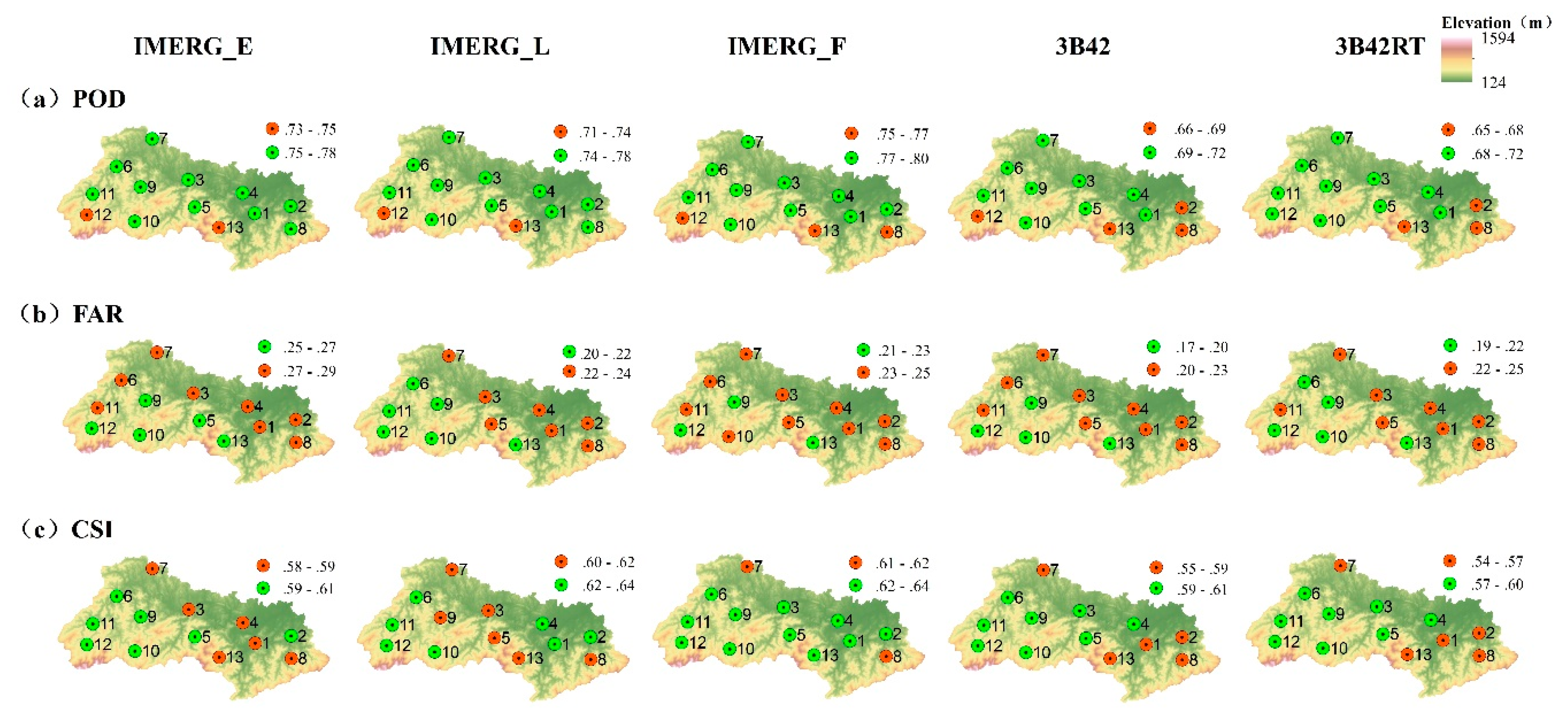
Figure A5 compares the spatial distribution of the three annual categorical evaluation metrics among the SPPs. Unlike the case of continuous metrics, topography does not seem to impose a consistent impact on categorical metrics at the daily scale. For example, while most SPPs have lower correct precipitation detection rates (PODs) at the two stations of high altitude (Station 12 and 13), they also have lower false alarm rates (FARs) at the stations. The leads to no obvious pattern in the spatial distribution of CSIs, with varied performance of stations at similar altitudes.

(3) Variation with Rainfall Thresholds

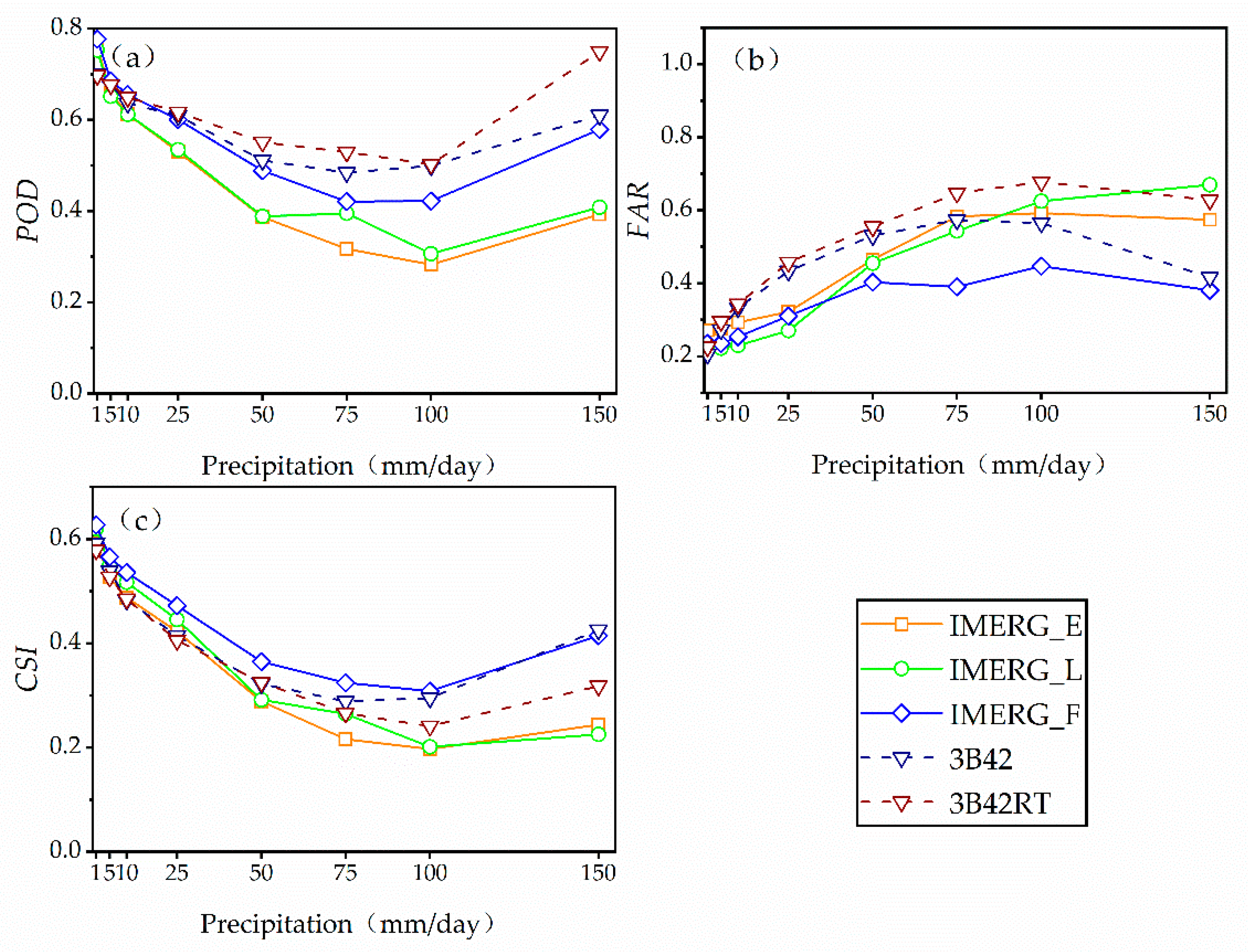
Figure 6 compares the performance of precipitation detection among the five SPPs by different daily rainfall magnitude. Each of the three categorical metrics has been sequentially calculated annually for the days when daily rainfall exceeds 1, 5, 10, 25, 50, 75, 100, and 150 mm/d. Similar daily rainfall thresholds have been used in previous studies, such as Wu et al. [29], Anjum et al. [43], and Tan et al. [49].
As seen from Figure 6a, the PODs of all five SPPs exhibit a largely decreasing trend with the increase of daily rainfall threshold until hitting the bottom at the threshold of 100 mm/d. Afterwards, the PODs of all SPPs bounce back substantially at the threshold of 150 mm/d. Interestingly, the PODs of the two TMPA products have mostly surpassed those of the IMERG products, indicating their better capabilities of correctly detecting daily rainfall occurrences.
However, as shown in Figure 6b, the FAR values of the TMPA products have also surpassed those of the IMERG products, especially IMERG_F, at the majority of daily rainfall thresholds, indicating their higher risk of falsely detecting daily rainfall occurrences. By incorporating the factors of both false alarms and missed events, CSI provides a more comprehensive evaluation of precipitation rainfall detection performance of the SPPs. As shown in Figure 6c, the IMERG_F has the highest CSI value at the daily rainfall thresholds of less than 100 mm/d, whereas it is caught up by the 3B42 at the threshold of 100 mm/d and above.

4.2.3. Comparison with Previous Studies

Table 5 summarizes the performance of the SPPs in estimating daily rainfall in previous studies worldwide. Previous studies have mostly assessed SPPs over approximately two years, compared to nine years in this study. It needs to be noted that the table does not serve to rigorously compare the relative performance of the SPPs in various regions, due to the differences in temporal frame, geographical regions, as well as climatic regimes of the studies.
The CCs of both IMERG products and TMPA products in this study have surpassed those in all previous studies except the one by Su et al. [46] conducted in the Upper Huai River Basin of China. Unlike the CC, the values of the other continuous as well as categorical metrics in this study all lie at the medium level among the previous studies. In addition, similar to our findings, many of previous studies have concluded a moderately better performance of the IMERG products in estimating daily rainfall than the TMPA products. However, the observed tendency of under-estimating daily rainfall by the IMERG products and over-estimating by the TMPA products in this study is not consistent with the findings of some previous studies.

4.3. Evaluation at the Hourly Scale

Figure A6 compares the scatterplots between observed and estimated hourly rainfall among the SPPs. Hourly rainfall estimates by all five SPPs are much scattered around the 1:1 line. Since hourly rainfall is only recorded from April to October, we evaluate the performance of the SPPs at the hourly scale for these seven months. Correspondingly, seasonal evaluation metrics are only calculated for spring (April to May), summer (June to August), and fall (September to October).

4.3.1. Continuous Evaluation Metrics

(1) Temporal Variation

Table 6 compares the mean values of the four continuous (CC, RMSE, RB, and MAD) over the seven months from April to October and seasonally (spring, summer, fall) among the SPPs at the hourly scale. With their seven-month CC values all staying close to 0.5, SPPs have performed less satisfactorily in estimating hourly rainfall in the SRB.
All IMERG products tend to underestimate hourly rainfall throughout the three seasons. The absolute RBs of IMERG_F are all below 13%, while those of the near-real-time products remain above 20%. With the smallest absolute RB among the SPPs, 3B42 tends to slightly overestimate daily rainfall in spring, but underestimate in summer and fall. Different from the other SPPs, 3B42RT shows a strong tendency of overestimation in summer.
Except for RB, the five SPPs all exhibit similar season patterns of change. Seasonally, the CCs of the SPPs all peak in spring followed by a continuous decline in summer and fall. Both the RMSEs and MADs of the SPPs are the highest in summer, followed by spring and then fall. The observed seasonal patterns at the hourly scale are quite similar to those observed at the daily scale.
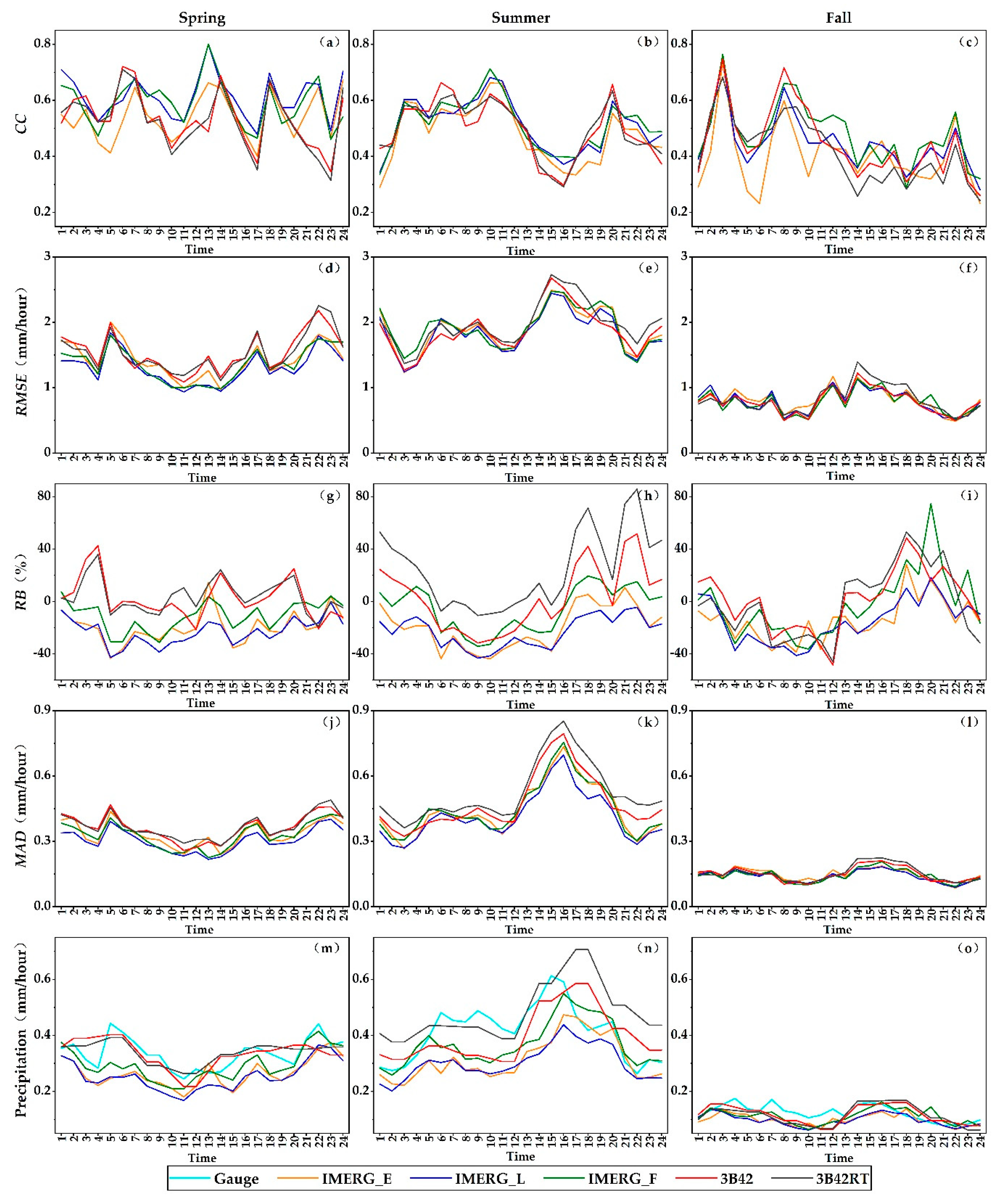
Figure 7a to Figure 7l further examine the changes in mean continuous metrics over a diurnal cycle in three seasons. Meanwhile, Figure 7m to Figure 7o compare the observed amount of average hourly rainfall with the corresponding SPP estimates in the three seasons. The CCs of all five SPPs have shown considerable diurnal variations in the three seasons. Despite the differences in amount, the overall diurnal patterns of change in CCs are somewhat similar among the SPPs. In summer, for example, the CCs of all SPPs tend to reach a high plateau between 3:00 a.m. and 12:00 p.m., followed by a steady fall to the bottom at around 4:00 p.m. and a rebound afterwards. As shown in Figure 7n, mean hourly summer ground measurement peaks at 3:00 p.m. All SPPs, however, have exhibited a lag of one or more hours in reaching the peak value, which may have caused their CCs all drop to the lowest in the afternoon. The diurnal patterns of change in RMSE/MAD are even more similar among the SPPs in all three seasons. Diurnal variations in both metrics are the highest in summer, followed by spring and then fall, which are consistent with the three seasons’ relative magnitude of diurnal changes in hourly precipitation (Figure 7m–o). In addition, the RMSEs and MADs of all five SPPs peak at 5:00 a.m., 5:00 p.m., and 10:00–11:00 p.m. in spring, and at 3:00–4:00 p.m. in summer. As seen from Figure 7m,n, hourly ground measurements also peak at these times.
The diurnal patterns of change in RB are more complex. Although differing much in their actual amount, the RBs of the five SPPs seem to follow a somewhat similar trend of change throughout the diurnal cycle, especially in summer. This is probably because rainfall estimates by the SPPs all exhibit a largely similar hourly trend in each season, in spite of the differences in their actual amount. Nevertheless, precisely because of the difference in their actual RB amount, the five SPPs give quite different estimation performance across the diurnal cycle. For example, 3B42RT tend to overestimate hourly rainfall most seriously at night (6:00 p.m. and 9:00–10:00 p.m.), while giving the estimates with the least bias in the morning. In contrast, IMERG products tend to underestimate rainfall mostly seriously in the morning (8:00–11:00 a.m.), but give the estimates with the least bias at night (7:00–10:00 p.m.) (Figure 7).
In addition, the relative performance of the SPPs at the hourly scale is somewhat different from that at the monthly and daily scales. In general, there is much less variability in the performance of the SPPs at the hourly scale compared to that at the monthly and daily scales. Except for RB, only two IMERG products (IMERG_F and IMERG_L) have slightly outperformed the TMPA products for most of the time.
To date, only limited studies have evaluated the quality of the hourly rainfall estimates of the SPPs. Similar to our study, they have mostly found that the performance of SPPs in estimating hourly rainfall was less satisfactory. For example, Caracciolo et al. [53] calculated the CCs to be respectively 0.32 and 0.26 when using the IMERG_F V4 for estimating hourly rainfall in Sardinia and Sicily of Italy. Li et al. [54] evaluated the performance of IMERG_F in estimating hourly rainfall in the Ganjiang River Basin of China, and calculated its CC, RMSE, and RB to be 0.33, 1.72 mm/h, and 0.12%, respectively. Yuan et al. [55] evaluated the 3-hour rainfall estimates by the three IMERG and two TMPA products in the Chindwin River basin, Myanmar, and they found that IMERG_F performed best with a CC of 0.33 and RB of −6.8%. Meanwhile, the RMSEs of the SPPs were similar, ranging from 2.9 to 3.1 mm/h.

(2) Statistical Performance Comparison among the SPPs

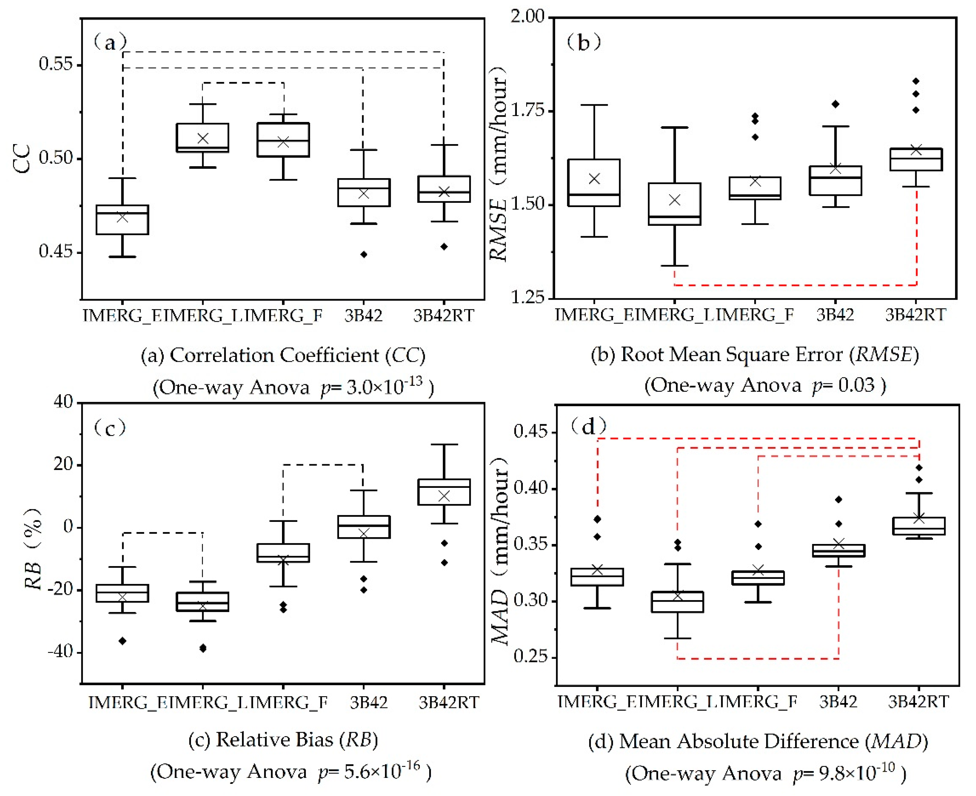
Figure 8 compares the boxplots of the four continuous evaluation metrics (April to October) at the hourly scale among the SPPs. For example, Figure 8b contains five boxplots, which respectively characterize the distribution of RMSEs (April to October) of the five SPPs across the 13 rainfall stations. The RMSEs of the IMERG_E range from 1.42 to 1.77 among the 13 rainfall stations, compared to 1.34–1.71 for IMERG_L, 1.45–1.74 for IMERG_F, 1.49–1.77 for 3B42, and 1.55–1.83 for 3B42RT.
Levene’s Test has confirmed that all four metrics could meet the pre-condition of homogeneity of variance for conducting one-way ANOVA. The subsequent one-way ANOVA has concluded that the mean values of all four metrics are significantly different among the SPPs at the significance level (α) of 0.05. Further posterior comparison tests have shown that the CCs are significantly different between most of the pairs of SPPs except four pairs (IMERG_L/IMERG_F; IMERG_E/3B42; IMERG_E/3B42RT; and 3B42/3B42RT), while the RBs are significantly different except between two pairs (IMERG_E/IMERG_L and IMERG_F/3B42). Unlike CC and RB, the RMSEs of the SPPs are only significantly different between one pair (IMERG_L/3B42RT). Finally, the MADs are only significantly different between 3B42RT and all IMERG products, as well as between 3B42 and IMERG_L (Figure 8). It is worth noting that the posterior comparison tests have shown that IMERG_F is not significantly different from the TMPA products in terms of all four metrics except CC.

(3) Spatial Variation

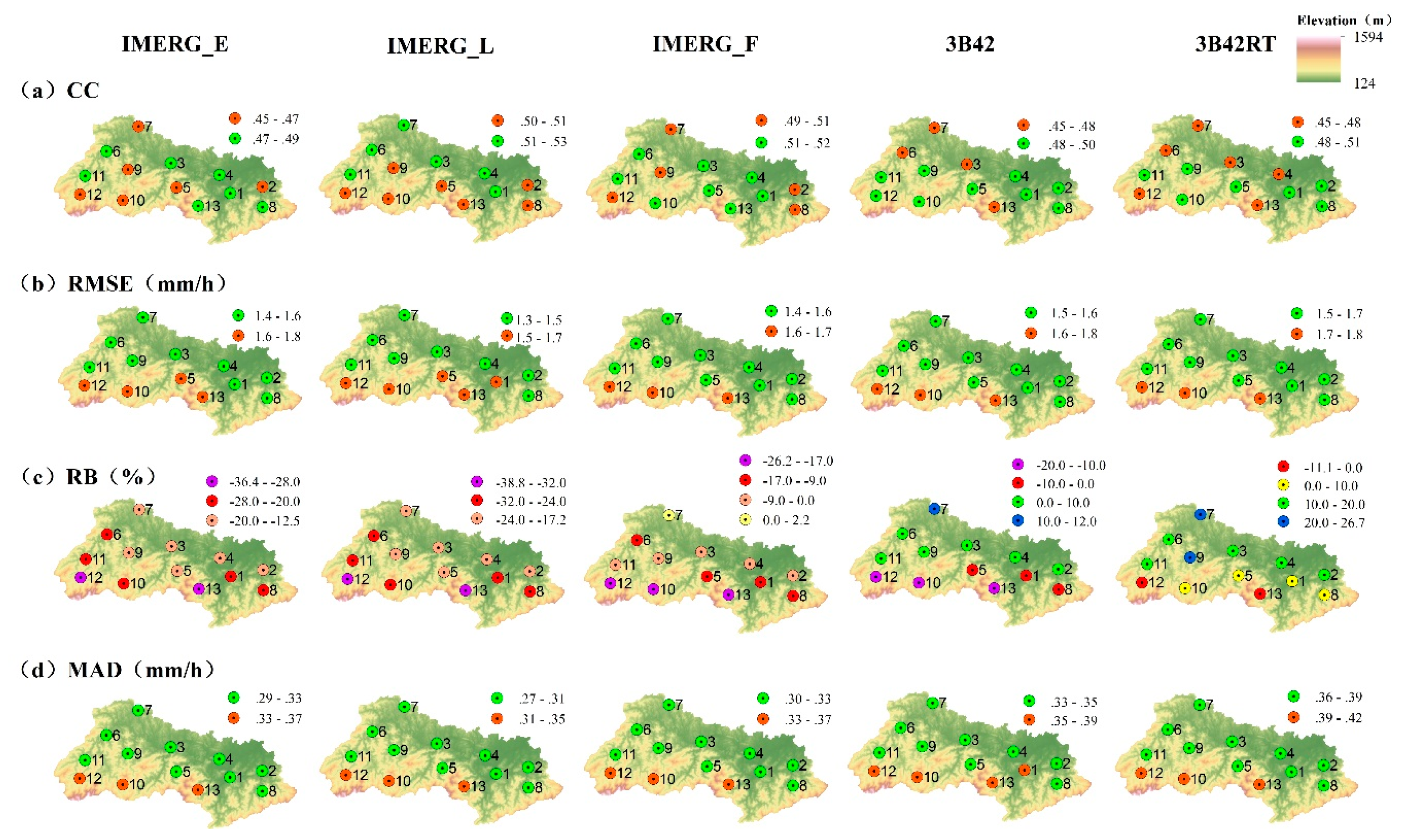
Figure 9 compares the spatial distribution of the four annual continuous evaluation metrics among the SPPs. At the hourly scale, topography also does not seem to be a significant influencing factor of the CCs, with lower CC values observed at stations of both low and high altitude. However, the spatial distribution of the other three metrics does indicate a significant impact of topography on the performance of the SPPs in estimating hourly rainfall. Both RMSEs and MADs exhibit similar spatial patterns across the five SPPs, whose values at the three stations of high altitude (station 10, 12, and 13) consistently stay at the top. As discussed above, the IMERG products tend to underestimate hourly rainfall. As shown in Figure 9, underestimation by the IMERG products is especially severe at higher altitude. Meanwhile, the 3B42 product also tends to underestimate hourly rainfall more at high altitude. Different from the other SPPs, the 3B42RT product tends to overestimate hourly rainfall more seriously at lower altitude.

4.3.2. Categorical Evaluation Metrics

(1) Temporal Variation

Table 7 compares the mean values of the three categorical metrics (POD, FAR, and CSI) over the seven months from April to October and seasonally (spring, summer, fall) among the SPPs at the hourly scale. Similar to the daily scale, three categorical metrics are used to assess the hourly precipitation detection capabilities of the SPPs. An hourly rainfall threshold of 0.1 mm/d is used in calculating the metrics. As seen from the table, with lower PODs and CSIs, as well as higher FARs, all five SPPs are poorer at detecting hourly rainfall than daily rainfall.
Seasonally, the five SPPs have exhibited somewhat similar patterns of change in hourly rainfall detection performance. In summer, they all have the highest correct rainfall detection rates (PODs), but also the highest false alarm rates (FARs). Between the rest two seasons, all five SPPs have higher PODs as well as lower FARs, therefore better rainfall detection performance, in spring. In fact, the seasonal CSIs indicate that the overall rainfall detection performance of the SPPs all tops in spring, followed by summer, and then winter.
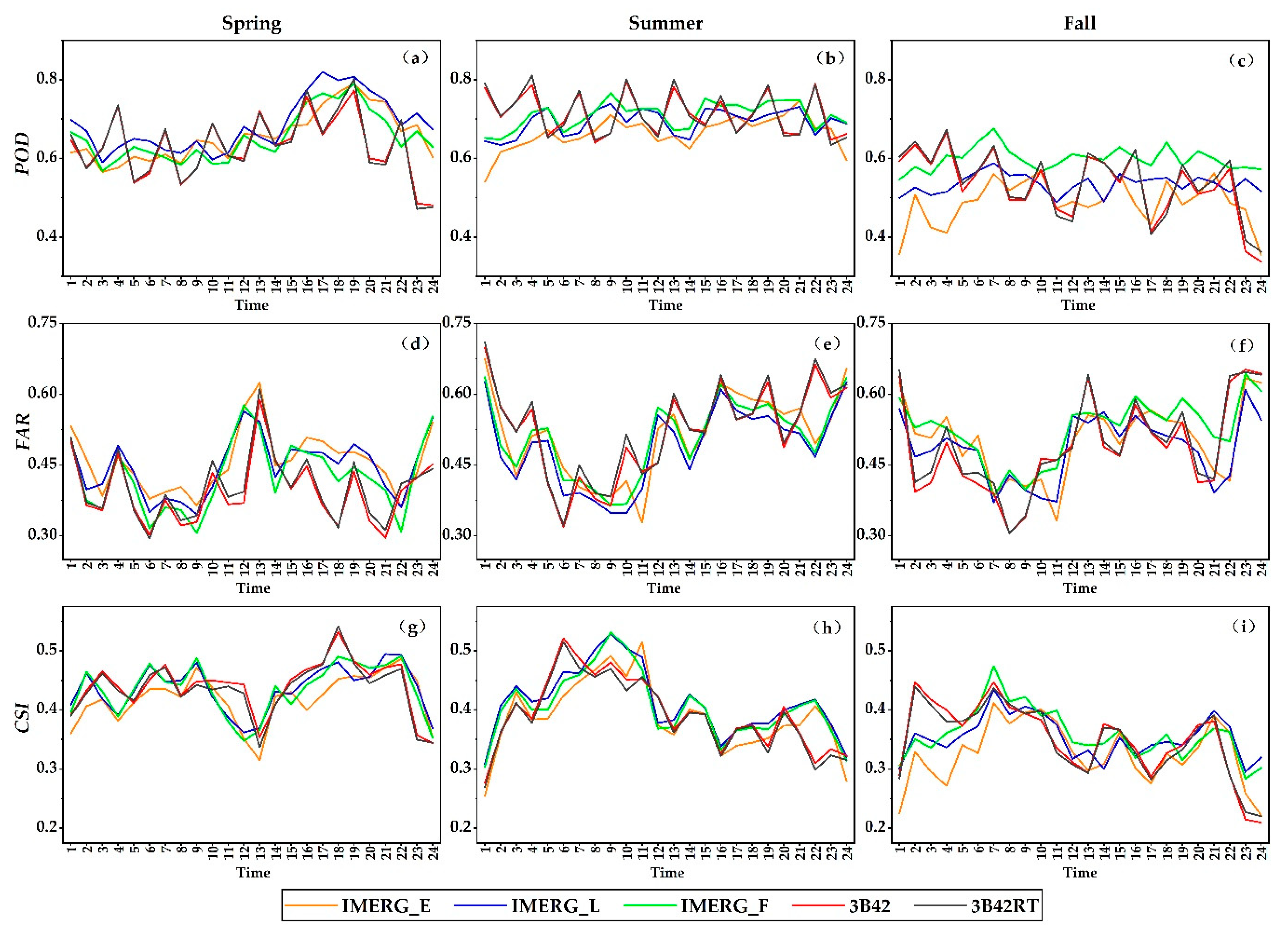
Figure 10 further examines the changes in mean categorical metrics over a diurnal cycle in three seasons. Among the three categorical metrics, PODs, especially those of IMERG_L and IMERG_F, exhibit relatively less hourly variations through the diurnal cycle. The only discernible pattern in the metric is that the IMERG products tend to have the highest correct rainfall detection rates (> 0.7) in early evening, while the TMPA products have the lowest at midnight in spring. Unlike POD, FAR exhibits more diurnal variations. In spring, FARs of all five SPPs tend to peak around noon. Whereas, in summer and fall, they all tend to bottom in the morning and climb to the peak at around midnight. Similar to FAR, CSI exhibits distinct diurnal variations. In spring, all SPPs have the lowest CSI, i.e., the poorest hourly rainfall detection performance at noon and midnight. In summer and fall, the performance of the SPPs tends to peak in the morning, and bottom out around midnight.
Similar to the results of the continuous metrics at the hourly scale, the values of all three categorical metrics are not much different among the SPPs, indicating the IMERG products are no longer superior to the TMPA products in hourly rainfall detection.
The values of the categorical metrics obtained in this study lie at the medium level among those obtained in previous limited studies. For example, Omranian and Sharif [56] evaluated the Early, Late, and Final runs of IMERG products for May 2015 in the Lower Colorado River Basin of Texas in U.S. At the hourly scale, they obtained a POD value of 0.74, a FAR value of 0.45 and a CSI value of 0.46. However, in their evaluation of the 3-hour daytime satellite rainfall estimates in the Chindwin River basin, Myanmar, Yuan et al. [55] obtained a POD value of <0.3 for all three IMERG and two TMPA products.

(2) Spatial Variation

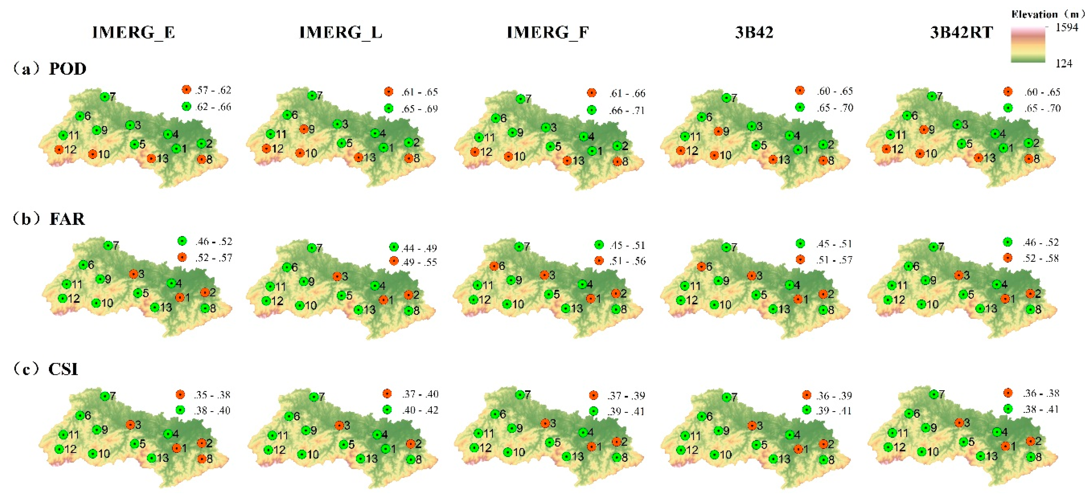
Figure A7 compares the spatial distribution of the three annual categorical evaluation metrics among the SPPs. At the hourly scale, the spatial distribution of the categorical metrics exhibits a similar pattern across the five SPPs. All five SPPs are poorer at detecting the actual precipitation occurrences at high altitude. However, they also tend to yield more false alarms at low altitude. The conflicting impacts of elevation on the PODs and FARs of the SPPs have led to lower CSI values, i.e., worse overall hourly precipitation detection performance, at the lower altitude, especially at stations 1–3.

(3) Variation with Rainfall Thresholds

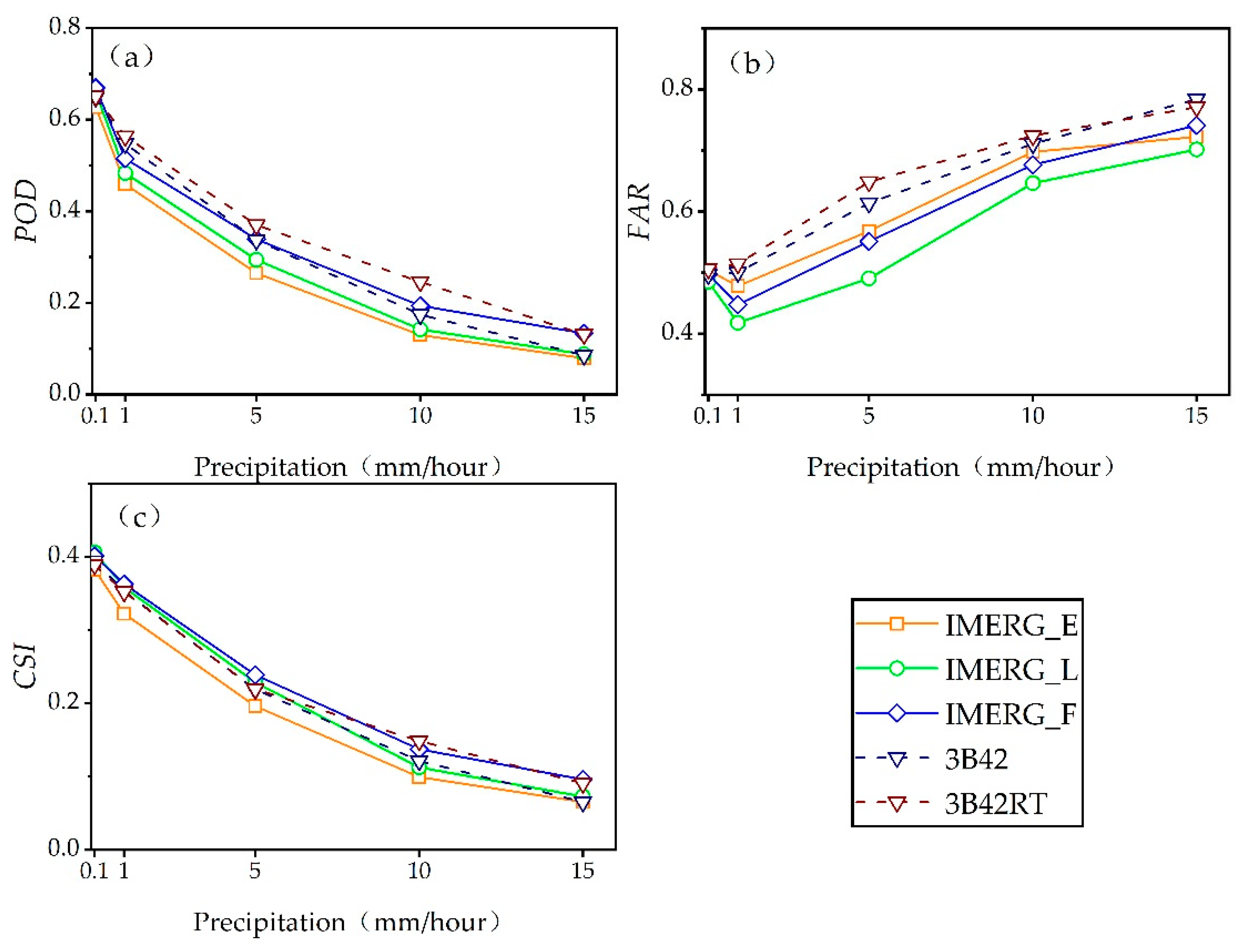
Figure 11 compares the performance of hourly precipitation detection among the five SPPs by different rainfall magnitude. Each of the three categorical metrics has been sequentially calculated when hourly rainfall exceeds 0.1, 1, 5, 10, and 15 mm. As seem from Figure 11a, the PODs of the five SPPs have all decreased steadily with increasing hourly rainfall thresholds before plunging to nearly 0 at the threshold of 15 mm/hour. In general, the five SPPs do not differ much in their PODs across the entire range of hourly rainfall thresholds. The PODs of the two near-real-time IMERG products are consistently less than those of the TMPA products. The PODs of 3B42RT have actually remained at or nearly the top across the rainfall thresholds.
As seem from Figure 11b, the FARs of all five SPPs tend to rise with increasing rainfall thresholds. The TMPA products have consistently yielded higher FARs than the IMERG products over the entire range of rainfall thresholds. The more comprehensive CSI values have concluded much similar hourly rainfall detection performance among the SPPs across the rainfall thresholds, with IMERG_F staying at or near the top most of the time (Figure 11c).

5. Conclusions

SPPs have increasingly become an important data source for precipitation inputs in hydrological modeling and other related studies worldwide. For local regions with scarce precipitation observations or limited access to precipitation data, the latest GPM and TRMM products provide a valuable alternative for obtaining the much-needed rainfall inputs for various regional hydrological applications. However, the accuracy of their rainfall estimates should be systematically assessed before being utilized in real world applications. In this study, we have assessed and compared the accuracy of the latest five GPM IMERG V6 and TRMM 3B42 V7 precipitation products across the monthly, daily, and hourly scales in a middle-sized hilly river basin in eastern central China. For evaluation, a total of four continuous and three categorical metrics have been calculated based on SPP estimates and historical rainfall records at 13 stations over a period of 9 years from 2009 to 2017. The evaluation results have led to the following main conclusions:
(1)
Rainfall estimates by all five SPPs could match ground observations best at the monthly scale, followed by the daily and hourly scale. The annual CCs of the SPPs, for example, have fallen from 0.86 or above at the monthly scale to mostly around 0.75 at the daily scale, and sharply to less than 0.6 (April to October) at the hourly scale. Topography tends to impose similar impact on the performance of SPPs across various time scales, with more estimation deviations at high altitude.
(2)
For estimating monthly rainfall, IMERG_F performs the best, closely followed by 3B42. These two post-time SPPs produce considerably better monthly rainfall estimates than the rest real-time or near-real-time SPPs. All three IMERG products tend to underestimate monthly rainfall except a slight overestimation by the two near-real-time products in winter. Meanwhile, 3B42RT exhibits a strong tendency to overestimate in summer and winter.
(3)
For estimating daily rainfall, the IMERG products generally perform better than the TMPA products, with IMERG_F performing the best. Similar to the monthly scale, the IMERG family products tend to underestimate daily rainfall in all four seasons except the two near-real-time products in winter. In contrast, 3B42RT exhibits a strong tendency of overestimation in summer and winter. In terms of rainfall detection performance, the TMPA products are more capable of correctly detecting daily rainfall occurrences, while the IMERG products contain fewer false detections of rainfall occurrences.
(4)
For estimating hourly rainfall, the performance of the SPPs is much more homogeneous. Two IMERG products (IMERG_F and IMERG_L) have slightly outperformed the TMPA products for most of the time. All IMERG products tend to underestimate hourly rainfall throughout the three seasons between April and October. In contrast, 3B42RT shows a strong tendency of overestimation in summer. In addition, the performances of hourly rainfall detection are quite similar among the five SPPs.
In general, our nine-year systematic evaluation of the latest GPM IMERG V6 and TRMM 3B42 V7 precipitation products have shown that the SPPs, especially the post-time IMERG_F product, could be considered as a reliable data source for providing monthly or daily rainfall data for regional hydrological applications. However, great caution needs to be exerted to utilize the hourly rainfall SPPs considering their overall weak correlations with ground rainfall observations, as well as the consistent tendency of underestimation by the IMERG products.
Hourly rainfall datasets have been increasingly found to be valuable inputs to a variety of hydrological applications. However, limited access to hourly rainfall datasets have restrained such applications in many regions. Owing to their wide spatial coverage and open access, SPPs have great potential to act as a useful alternative source for providing hourly rainfall data. Therefore, effective bias-correction algorithms incorporating ground rainfall observations are needed to improve the quality of hourly rainfall SPPs to safeguard the validity of their usage as ground measurement surrogates.

Author Contributions

Conceptualization, X.Y. and M.L.T.; Methodology, X.Y. and R.H.; Software, Y.L. and X.L.; Validation, X.Y. and G.W.; Formal analysis, X.Y. and Y.L.; Investigation, X.Y. and Y.L.; Resources, G.W. and R.H.; Data curation, Y.L. and X.L.; Writing—original draft preparation, X.Y. and Y.L.; Writing—review and editing, M.L.T., G.W., and R.H.; Visualization, Y.L. and X.L.; Supervision, X.Y. and R.H.; Project administration, X.Y. and R.H.; Funding acquisition, R.H. and X.Y. All authors have read and agreed to the published version of the manuscript.

Funding

This research was funded by the Belt and Road Special Foundation of the State Key Laboratory of Hydrology—Water Resources and Hydraulic Engineering at Nanjing Hydraulic Research Institute, China, grant number 2018nkzd01; National Natural Science Foundation of China, grant number 41830863 and 51679144; National Key Research and Development Program of China, grant number 2016YFA0601501; the Ministry of Education, Malaysia under the NEWTON-NERC grant (IMpacts of PRecipitation from Extreme StormS—Malaysia (IMPRESS-MALAYSIA), grant number 203.PHUMANITI.6780001; and Fundamental Research Grant Scheme, grant number 203.PHUMANITI.6711695. The APC was funded by the Belt and Road Special Foundation of the State Key Laboratory of Hydrology—Water Resources and Hydraulic Engineering at Nanjing Hydraulic Research Institute, China, grant number 2018nkzd01.

Conflicts of Interest

The authors declare no conflict of interest.

Appendix A

Figure A1. Mean annual precipitation in the Shuaishui River Basin: 2009–2017. The error bar shows ± one standard deviation of the annual average precipitation among the 13 rainfall stations.
Remotesensing 12 01042 g0a1
Figure A2. Mean monthly precipitation in the Shuaishui River Basin: 2009–2017. The error bar shows ± one standard deviation of the monthly average precipitation among the 13 stations.
Remotesensing 12 01042 g0a2
Figure A3. Scatterplots between monthly rainfall gauge observations and satellite precipitation product estimates.
Remotesensing 12 01042 g0a3
Figure A4. Scatterplots between daily rainfall gauge observations and satellite precipitation product estimates.
Remotesensing 12 01042 g0a4
Figure A5. Spatial distribution of the annual categorical evaluation metrics at daily scale: (a) POD; (b) FAR; and (c) CSI.
Remotesensing 12 01042 g0a5
Figure A6. Scatterplots between hourly rainfall gauge observations and satellite precipitation product estimates.
Remotesensing 12 01042 g0a6
Figure A7. Spatial distribution of the categorical evaluation metrics (April to October) at hourly scale: (a) POD; (b) FAR; and (c) CSI.
Remotesensing 12 01042 g0a7

References

  1. Wu, P.; Christidis, N.; Stott, P. Anthropogenic impact on Earth’s hydrological cycle. Nat. Clim. Chang. 2013, 3, 807–810. [Google Scholar] [CrossRef]
  2. Allen, M.R.; Ingram, W.J. Constraints on future changes in climate and the hydrologic cycle. Nature 2012, 489, 590. [Google Scholar] [CrossRef] [Green Version]
  3. Lee, J.; Lee, E.-H.; Seol, K.-H. Validation of Integrated MultisatellitE Retrievals for GPM (IMERG. by using gauge-based analysis products of daily precipitation over East Asia. Theor. Appl. Climatol. 2019, 137, 2497–2512. [Google Scholar] [CrossRef]
  4. Hou, A.Y.; Kakar, R.K.; Neeck, S.; Azarbarzin, A.A.; Kummerow, C.D.; Kojima, M.; Oki, R.; Nakamura, K.; Iguchi, T. The global precipitation measurement mission. Bull. Am. Meteorol. Soc. 2014, 95, 701. [Google Scholar] [CrossRef]
  5. Shen, Y.; Xiong, A. Validation and comparison of a new gauge-based precipitation analysis over mainland China. Int. J. Climatol. 2016, 36, 252–265. [Google Scholar] [CrossRef]
  6. Tan, M.L.; Ibrahim, A.; Duan, Z.; Cracknell, A.P.; Chaplot, V. Evaluation of six high-resolution satellite and ground-based precipitation products over Malaysia. Remote Sens. 2015, 7, 1504–1528. [Google Scholar] [CrossRef] [Green Version]
  7. Tancreto, A.E. Comparison of Hydrologic Model Performance Statistics Using Thiessen Polygon Rain Gauge and NEXRAD Precipitation Input Methods at Different Watershed Spatial Scales and Rainfall Return Frequencies; University of North Florida: Jacksonville, FL, USA, 2015; Available online: https://digitalcommons.unf.edu/etd/584 (accessed on 23 March 2020).
  8. Louf, V.; Protat, A.; Warren, R.A.; Collis, S.M.; Wolff, D.B.; Raunyiar, S.; Jakob, C.; Petersen, W.A. An integrated approach to weather radar calibration and monitoring using ground clutter and satellite comparisons. J. Atmos. Ocean. Technol. 2019, 36, 17–39. [Google Scholar] [CrossRef] [Green Version]
  9. Letu, H.; Nagao, T.M.; Nakajima, T.Y.; Riedi, J.; Ishimoto, H.; Baran, A.J.; Shang, H.; Sekiguchi, M.; Kikuchi, M. Ice cloud properties from Himawari-8/AHI next-generation geostationary satellite: Capability of the AHI to monitor the DC cloud generation process. IEEE Trans. Geosci. Remote Sens. 2019, 57, 3229–3239. [Google Scholar] [CrossRef]
  10. Rutledge, S.A.; Chandrasekar, V.; Fuchs, B.; George, J.; Junyent, F.; Kennedy, P.; Dolan, B. Deployment of the SEA-POL C-band Polarimetric Radar to SPURS-2. Oceanography 2019, 32, 50–57. [Google Scholar] [CrossRef]
  11. Beck, H.E.; Pan, M.; Roy, T.; Weedon, G.P.; Pappenberger, F.; van Dijk, A.I.J.M.; Huffman, G.J.; Adler, R.F.; Wood, E.F. Daily evaluation of 26 precipitation datasets using Stage-IV gauge-radar data for the CONUS. Hydrol. Earth Syst. Sci. 2019, 23, 207–224. [Google Scholar] [CrossRef] [Green Version]
  12. Joss, J.; Waldvogel, A.; Collier, C.G. Precipitation Measurement and Hydrology. In Radar in Meteorology: Battan Memorial and 40th Anniversary Radar Meteorology Conference; Atlas, D., Ed.; American Meteorological Society: Boston, MA, USA, 1990; pp. 577–606. [Google Scholar] [CrossRef]
  13. Dinku, T.; Anagnostou, E.N.; Borga, M. Improving radar-based estimation of rainfall over complex terrain. J. Appl. Meteorol. 2002, 41, 1163–1178. [Google Scholar] [CrossRef]
  14. Funk, C.; Peterson, P.; Landsfeld, M.; Pedreros, D.; Verdin, J.; Shukla, S.; Husak, G.; Rowland, J.; Harrison, L.; Hoell, A.; et al. The climate hazards infrared precipitation with stations-a new environmental record for monitoring extremes. Sci. Data 2015, 2. [Google Scholar] [CrossRef] [Green Version]
  15. Guo, H.; Chen, S.; Bao, A.; Hu, J.; Gebregiorgis, A.S.; Xue, X.; Zhang, X. Inter-comparison of high-resolution satellite precipitation products over Central Asia. Remote Sens. 2015, 7, 7181–7211. [Google Scholar] [CrossRef] [Green Version]
  16. Mantas, V.M.; Liu, Z.; Caro, C.; Pereira, A.J.S.C. Validation of TRMM multi-satellite precipitation analysis (TMPA) products in the Peruvian Andes. Atmos. Res. 2015, 163, 132–145. [Google Scholar] [CrossRef]
  17. Li, X.-H.; Zhang, Q.; Xu, C.-Y. Suitability of the TRMM satellite rainfalls in driving a distributed hydrological model for water balance computations in Xinjiang catchment, Poyang lake basin. J. Hydrol. 2012, 426, 28–38. [Google Scholar] [CrossRef]
  18. Bharti, V.; Singh, C. Evaluation of error in TRMM 3B42V7 precipitation estimates over the Himalayan region. J. Geophys. Res. -Atmos. 2015, 120, 12458–12473. [Google Scholar] [CrossRef]
  19. Tan, M.L.; Duan, Z. Assessment of GPM and TRMM precipitation products over Singapore. Remote Sens. 2017, 9, 720. [Google Scholar] [CrossRef] [Green Version]
  20. Sharifi, E.; Steinacker, R.; Saghafian, B. Assessment of GPM-IMERG and other precipitation products against gauge data under different topographic and climatic conditions in Iran: Preliminary results. Remote Sens. 2016, 8, 135. [Google Scholar] [CrossRef] [Green Version]
  21. Tang, G.; Ma, Y.; Long, D.; Zhong, L.; Hong, Y. Evaluation of GPM Day-1 IMERG and TMPA Version-7 legacy products over Mainland China at multiple spatiotemporal scales. J. Hydrol. 2016, 533, 152–167. [Google Scholar] [CrossRef]
  22. Suratman, S.; Aziz, A.A.; Tahir, N.M.; Lee, L.H. Distribution and behaviour of nitrogen compounds in the surface water of Sungai Terengganu Estuary, Southern Waters of South China Sea, Malaysia. Sains Malays. 2018, 47, 651–659. [Google Scholar] [CrossRef]
  23. Zhou, Y.; Wu, T. Composite analysis of precipitation intensity and distribution characteristics of western track landfall typhoons over China under strong and weak monsoon conditions. Atmos. Res. 2019, 225, 131–143. [Google Scholar] [CrossRef]
  24. Yang, X.; Warren, R.; He, Y.; Ye, J.; Li, Q.; Wang, G. Impacts of climate change on TN load and its control in a river basin with complex pollution sources. Sci. Total Environ. 2018, 615, 1155–1163. [Google Scholar] [CrossRef] [Green Version]
  25. Yang, X.; Liu, Q.; Fu, G.; He, Y.; Luo, X.; Zheng, Z. Spatiotemporal patterns and source attribution of nitrogen load in a river basin with complex pollution sources. Water Res. 2016, 94, 187–199. [Google Scholar] [CrossRef] [Green Version]
  26. Boithias, L.; Sauvage, S.; Lenica, A.; Roux, H.; Abbaspour, K.C.; Larnier, K.; Dartus, D.; Sanchez-Perez, J.M. Simulating flash floods at hourly time-step using the SWAT model. Water 2017, 9, 929. [Google Scholar] [CrossRef] [Green Version]
  27. Zhou, M.M.; Deng, J.S.; Lin, Y.; Belete, M.; Wang, K.; Comber, A.; Huang, L.Y.; Gan, M.Y. Identifying the effects of land use change on sediment export: Integrating sediment source and sediment delivery in the Qiantang River Basin, China. Sci. Total Environ. 2019, 686, 38–49. [Google Scholar] [CrossRef]
  28. Lin, Q.W.; Peng, X.; Liu, B.Y.; Min, F.L.; Zhang, Y.; Zhou, Q.H.; Ma, J.M.; Wu, Z.B. Aluminum distribution heterogeneity and relationship with nitrogen, phosphorus and humic acid content in the eutrophic lake sediment. Environ. Pollut. 2019, 253, 516–524. [Google Scholar] [CrossRef]
  29. Wu, Y.; Zhang, Z.; Huang, Y.; Jin, Q.; Chen, X.; Chang, J. Evaluation of the GPM IMERG V5 and TRMM 3B42 V7 precipitation products in the Yangtze River Basin, China. Water 2019, 11, 1459. [Google Scholar] [CrossRef] [Green Version]
  30. Zhao, H.; Yang, S.; Wang, Z.; Zhou, X.; Luo, Y.; Wu, L. Evaluating the suitability of TRMM satellite rainfall data for hydrological simulation using a distributed hydrological model in the Weihe River catchment in China. J. Geogr. Sci. 2015, 25, 177–195. [Google Scholar] [CrossRef]
  31. Beaufort, A.; Gibier, F.; Palany, P. Assessment and correction of three satellite rainfall estimate products for improving flood prevention in French Guiana. Int. J. Remote Sens. 2019, 40, 171–196. [Google Scholar] [CrossRef]
  32. Huffman, G.J.; Adler, R.F.; Bolvin, D.T.; Gu, G.; Nelkin, E.J.; Bowman, K.P.; Hong, Y.; Stocker, E.F.; Wolff, D.B. The TRMM multisatellite precipitation analysis (TMPA): Quasi-global, multiyear, combined-sensor precipitation estimates at fine scales. J. Hydrometeorol. 2007, 8, 38–55. [Google Scholar] [CrossRef]
  33. Real-Time TRMM Multi-Satellite Precipitation Analysis Data Set Documentation. Available online: https://pmm.nasa.gov/sites/default/files/document_files/3B4XRT_doc_V7_180426.pdf (accessed on 17 March 2020).
  34. Bushair, M.T.; Kumar, P.; Gairola, R.M. Evaluation and assimilation of various satellite-derived rainfall products over India. Int. J. Remote Sens. 2019, 40, 5315–5338. [Google Scholar] [CrossRef]
  35. Algorithm Theoretical Basis Document (ATBD) Version 06. NASA Global Precipitation Measurement (GPM) Integrated Multi-satellitE Retrievals for GPM (IMERG). Available online: https://pmm.nasa.gov/sites/default/files/document_files/IMERG_ATBD_V06.pdf (accessed on 17 March 2020).
  36. Yong, B.; Ren, L.; Hong, Y.; Gourley, J.J.; Tian, Y.; Huffman, G.J.; Chen, X.; Wang, W.; Wen, Y. First evaluation of the climatological calibration algorithm in the real- time TMPA precipitation estimates over two basins at high and low latitudes. Water Resour. Res. 2013, 49, 2461–2472. [Google Scholar] [CrossRef] [Green Version]
  37. Condom, T.; Rau, P.; Espinoza, J.C. Correction of TRMM 3B43 monthly precipitation data over the mountainous areas of Peru during the period 1998–2007. Hydrol. Process. 2011, 25, 1924–1933. [Google Scholar] [CrossRef]
  38. Blacutt, L.A.; Herdies, D.L.; de Goncalves, L.G.G.; Vila, D.A.; Andrade, M. Precipitation comparison for the CFSR, MERRA, TRMM3B42 and Combined Scheme datasets in Bolivia. Atmos. Res. 2015, 163, 117–131. [Google Scholar] [CrossRef] [Green Version]
  39. El Kenawy, A.M.; Lopez-Moreno, J.I.; McCabe, M.F.; Vicente-Serrano, S.M. Evaluation of the TMPA-3B42 precipitation product using a high-density rain gauge network over complex terrain in northeastern Iberia. Glob. Planet. Chang. 2015, 133, 188–200. [Google Scholar] [CrossRef] [Green Version]
  40. Yong, B.; Ren, L.-L.; Hong, Y.; Wang, J.-H.; Gourley, J.J.; Jiang, S.-H.; Chen, X.; Wang, W. Hydrologic evaluation of multisatellite precipitation analysis standard precipitation products in basins beyond its inclined latitude band: A case study in Laohahe basin, China. Water Resour. Res. 2010, 46. [Google Scholar] [CrossRef] [Green Version]
  41. Gerapetritis, H.; Pelissier, J. The critical success index and warning strategy. In Proceedings of the 17th Conference on Probablity and Statistics in the Atmospheric Sciences, Seattle, WC, USA, 11–15 January 2004. [Google Scholar]
  42. Chen, S.; Hong, Y.; Cao, Q.; Gourley, J.J.; Kirstetter, P.-E.; Yong, B.; Tian, Y.; Zhang, Z.; Shen, Y.; Hu, J.; et al. Similarity and difference of the two successive V6 and V7 TRMM multisatellite precipitation analysis performance over China. J. Geophys. Res. -Atmos. 2013, 118, 13060–13074. [Google Scholar] [CrossRef]
  43. Anjum, M.N.; Ding, Y.; Shangguan, D.; Ahmad, I.; Ijaz, M.W.; Farid, H.U.; Yagoub, Y.E.; Zaman, M.; Adnan, M. Performance evaluation of latest integrated multi-satellite retrievals for Global Precipitation Measurement (IMERG) over the northern highlands of Pakistan. Atmos. Res. 2018, 205, 134–146. [Google Scholar] [CrossRef]
  44. Yang, M.; Li, Z.; Anjum, M.N.; Gao, Y. Performance Evaluation of Version 5 (V05) of Integrated Multi-Satellite Retrievals for Global Precipitation Measurement (IMERG) over the Tianshan Mountains of China. Water 2019, 11, 1139. [Google Scholar] [CrossRef] [Green Version]
  45. Milewski, A.; Elkadiri, R.; Durham, M. Assessment and comparison of TMPA satellite precipitation products in varying climatic and topographic regimes in Morocco. Remote Sens. 2015, 7, 5697–5717. [Google Scholar] [CrossRef] [Green Version]
  46. Su, J.; Lu, H.; Zhu, Y.; Cui, Y.; Wang, X. Evaluating the hydrological utility of latest IMERG products over the Upper Huaihe River Basin, China. Atmos. Res. 2019, 225, 17–29. [Google Scholar] [CrossRef]
  47. Wang, X.; Ding, Y.; Zhao, C.; Wang, J. Similarities and improvements of GPM IMERG upon TRMM 3B42 precipitation product under complex topographic and climatic conditions over Hexi region, Northeastern Tibetan Plateau. Atmos. Res. 2019, 218, 347–363. [Google Scholar] [CrossRef]
  48. Xu, F.; Guo, B.; Ye, B.; Ye, Q.; Chen, H.; Ju, X.; Guo, J.; Wang, Z. Systematical Evaluation of GPM IMERG and TRMM 3B42V7 Precipitation Products in the Huang-Huai-Hai Plain, China. Remote Sens. 2019, 11, 697. [Google Scholar] [CrossRef] [Green Version]
  49. Tan, M.L.; Santo, H. Comparison of GPM IMERG, TMPA 3B42 and PERSIANN-CDR satellite precipitation products over Malaysia. Atmos. Res. 2018, 202, 63–76. [Google Scholar] [CrossRef]
  50. Aslami, F.; Ghorbani, A.; Sobhani, B.; Esmali, A. Comprehensive comparison of daily IMERG and GSMaP satellite precipitation products in Ardabil Province, Iran. Int. J. Remote Sens. 2019, 40, 3139–3153. [Google Scholar] [CrossRef]
  51. Kim, K.; Park, J.; Baik, J.; Choi, M. Evaluation of topographical and seasonal feature using GPM IMERG and TRMM 3B42 over Far-East Asia. Atmos. Res. 2017, 187, 95–105. [Google Scholar] [CrossRef]
  52. Wang, W.; Lu, H.; Zhao, T.; Jiang, L.; Shi, J. Evaluation and comparison of daily rainfall from latest GPM and TRMM products over the Mekong River Basin. IEEE J. Sel. Top. Appl. Earth Obs. Remote Sens. 2017, 10, 2540–2549. [Google Scholar] [CrossRef]
  53. Caracciolo, D.; Francipane, A.; Viola, F.; Noto, L.V.; Deidda, R. Performances of GPM satellite precipitation over the two major Mediterranean islands. Atmos. Res. 2018, 213, 309–322. [Google Scholar] [CrossRef] [Green Version]
  54. Li, N.; Tang, G.; Zhao, P.; Hong, Y.; Gou, Y.; Yang, K. Statistical assessment and hydrological utility of the latest multi-satellite precipitation analysis IMERG in Ganjiang River basin. Atmos. Res. 2017, 183, 212–223. [Google Scholar] [CrossRef]
  55. Yuan, F.; Zhang, L.; Soe, K.M.W.; Ren, L.; Zhao, C.; Zhu, Y.; Jiang, S.; Liu, Y. Applications of TRMM- and GPM-Era multiple-satellite precipitation products for flood simulations at sub-daily scales in a sparsely gauged watershed in Myanmar. Remote Sens. 2019, 11, 140. [Google Scholar] [CrossRef] [Green Version]
  56. Omranian, E.; Sharif, H.O. Evaluation of the Global Precipitation Measurement (GPM) satellite rainfall products over the Lower Colorado River Basin, Texas. J. Am. Water Resour. Assoc. 2018, 54, 882–898. [Google Scholar] [CrossRef]
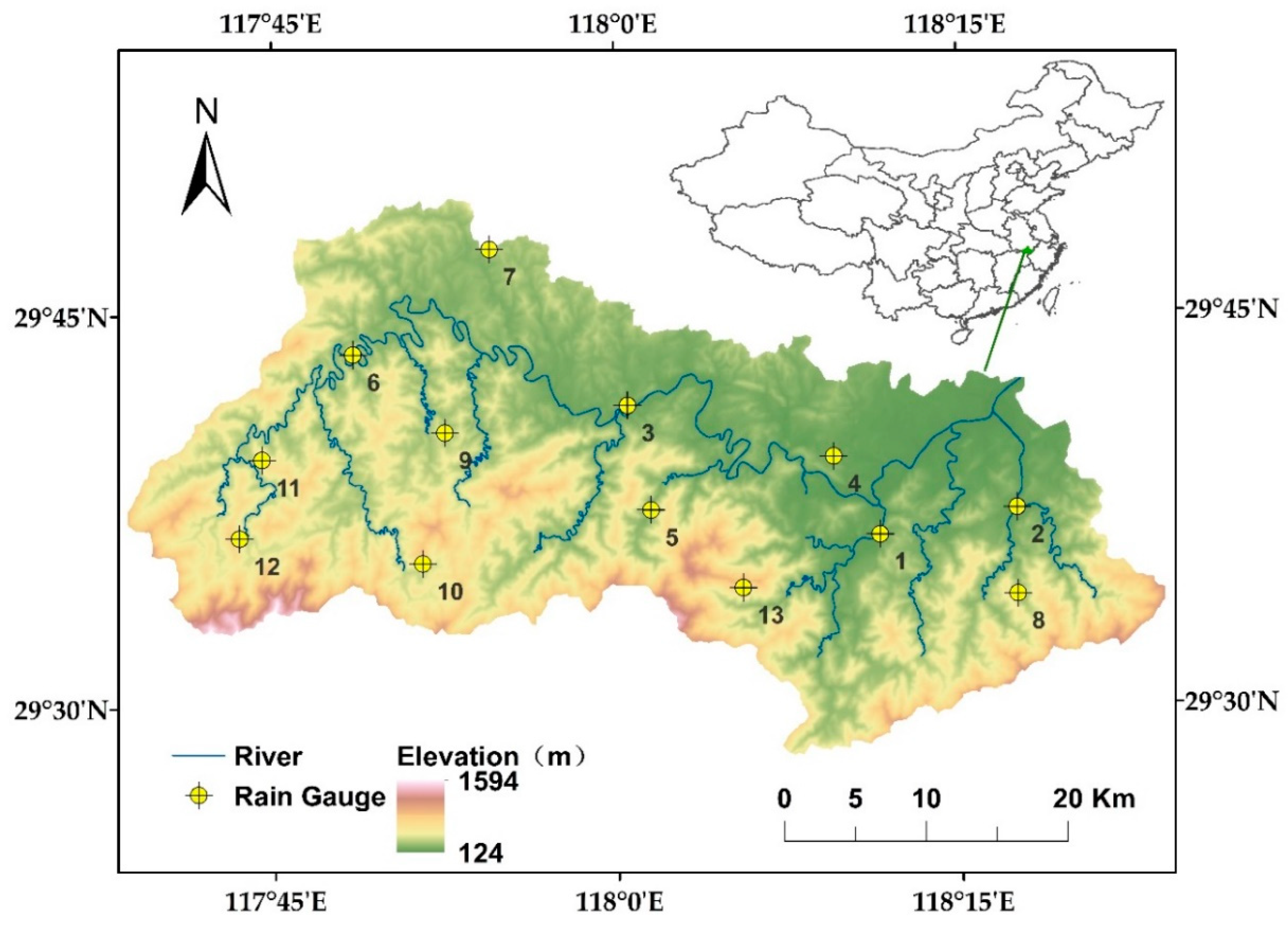
Figure 1. Map of Shuaishui River Basin.
Remotesensing 12 01042 g001
Figure 2. Comparison of mean monthly precipitation observations with the estimates of five SPPs from 2009 to 2017: (a) IMERG products; (b) TRMM products.
Remotesensing 12 01042 g002
Figure 3. Spatial distribution of the annual continuous evaluation metrics at monthly scale: (a) CC; (b) RMSE; (c) RB; and (d) MAD.
Remotesensing 12 01042 g003
Figure 4. Boxplots of the four annual continuous evaluation metrics of SPPs at daily scale: (a) Correlation coefficient (CC) (Levene’s Test, p = 0.08; One-Way ANOVA, p = 0.0); (b) Root-mean-square error (RMSE) (Levene’s Test, p = 0.16; One-Way ANOVA, p = 7.3 × 10⁻¹³); (c) Relative bias (RB) (Levene’s Test, p = 0.78; One-Way ANOVA, p = 3.2 × 10⁻¹³); and (d) Mean absolute difference (MAD) (Levene’s Test, p = 0.35; One-Way ANOVA, p = 3.0 × 10⁻¹⁵). Two SPPs are connected with a black dotted line if posterior comparison tests have concluded a non-significant difference between their means at α = 0.05. Each boxplot is used to depict the distribution, therefore the variation, of the continuous evaluation metrics among the 13 rainfall stations. In each boxplot, the top and bottom of the box represent the first and third quantiles. The whiskers extends to 1.5 times of the inter-quantile range. The horizontal line inside the box represents the median. The ‘×’ inside the box represents the mean.
Remotesensing 12 01042 g004
Figure 5. Spatial distribution of the annual continuous evaluation metrics at daily scale: (a) CC; (b) RMSE; (c) RB; and (d) MAD.
Remotesensing 12 01042 g005
Figure 6. Comparison of the changes in annual categorical evaluation metrics with daily rainfall thresholds among five SPPs: (a) POD; (b) FAR; and (c) CSI.
Remotesensing 12 01042 g006
Figure 7. Changes in mean continuous metrics over a diurnal cycle in three seasons: (a) CC in spring; (b) CC in summer; (c) CC in fall; (d) RMSE in spring; (e) RMSE in summer; (f) RMSE in fall; (g) RB in spring; (h) RB in summer; (i) RB in fall; (j) MAD in spring; (k) MAD in summer; (l) MAD in fall; (m) average observed and estimated hourly rainfall in spring; (n) average observed and estimated hourly rainfall in summer; and (o) average observed and estimated hourly rainfall in fall.
Remotesensing 12 01042 g007
Figure 8. Boxplots of the four continuous evaluation metrics (April to October) of SPPs at hourly scale: (a) correlation coefficient (CC) (Levene’s test, p = 0.77; one-way ANOVA, p = 3.0 × 10⁻¹³); (b) root-mean-square error (RMSE) (Levene’s test, p = 0.63; one-way ANOVA, p = 0.03); (c) relative bias (RB) (Levene’s test, p = 0.61; one-way ANOVA, p = 5.6 × 10⁻¹⁶); and (d) mean absolute difference (MAD) (Levene’s test, p = 0.87; one-way ANOVA, p = 9.8 × 10⁻¹⁰). For CC and RB, two SPPs are connected with a black dotted line if posterior comparison tests have indicated a non-significant difference between their means at α = 0.05. For RMSE and MAD, two SPPs are connected with a red dotted line if posterior comparison tests have indicated a significant difference between their means at α = 0.05. Each boxplot is used to depict the distribution, therefore the variation, of the continuous evaluation metrics among the 13 rainfall stations. In each boxplot, the top and bottom of the box represent the first and third quantiles. The whiskers extends to 1.5 times of the inter-quantile range. The horizontal line inside the box represents the median. The ‘×’ inside the box represents the mean.
Remotesensing 12 01042 g008
Figure 9. Spatial distribution of the continuous evaluation metrics (April to October) at hourly scale: (a) CC; (b) RMSE; (c) RB; and (d) MAD.
Remotesensing 12 01042 g009
Figure 10. Changes in mean categorical metrics over a diurnal cycle in three seasons: (a) POD in spring; (b) POD in summer; (c) POD in fall; (d) FAR in spring; (e) FAR in summer; (f) FAR in fall; (g) CSI in spring; (h) CSI in summer; and (i) CSI in fall.
Remotesensing 12 01042 g010
Figure 11. Comparison of the changes in categorical evaluation metrics (April to October) with hourly rainfall thresholds among five SPPs: (a) POD; (b) FAR; and (c) CSI.
Remotesensing 12 01042 g011
Table 1. Contingency table between rain gauge observations and satellite precipitation estimates.
SPPs EstimatesRain Gauge Observations
S ≥ ThresholdS < Threshold
P ≥ ThresholdHF
P < ThresholdMZ
Table 2. Mean evaluation metrics of the SPPs at monthly scale.
MetricsTemporal ScaleIMERG_EIMERG_LIMERG_F3B423B42RT
CCAnnual0.860.860.970.950.89
Spring a0.720.770.950.930.82
Summer a0.890.900.950.930.89
Fall a0.650.690.880.830.74
Winter a0.690.700.980.970.81
RMSE (mm)Annual86.6987.6453.8254.13101.42
Spring90.1789.5047.2344.0275.09
Summer118.98121.7187.1987.36170.08
Fall53.8852.5130.6435.7949.90
Winter67.1368.9325.1826.4161.58
RB (%)Annual−13.63−16.80−10.510.6110.69
Spring−13.74−19.33−12.00−0.02−4.91
Summer−19.13−22.71−9.85−1.4825.77
Fall−11.20−9.84−6.350.12−3.89
Winter0.790.15−11.889.6819.06
MAD (mm)Annual61.5961.7735.7937.0765.72
Spring71.8070.7237.9934.3460.64
Summer84.7887.9065.1765.30118.77
Fall43.5041.9723.1728.4040.75
Winter46.2846.4816.8320.2542.74
a Spring extends from March to May; Summer extends from June to August; Fall extends from September to November; Winter extends from December to the following February.
Table 3. Mean continuous evaluation metrics of the SPPs at daily scale.
MetricsTemporal ScaleIMERG_EIMERG_LIMERG_F3B423B42RT
CCAnnual0.730.750.810.750.75
Spring a0.710.770.790.740.73
Summer a0.800.810.830.780.77
Fall a0.640.650.730.700.68
Winter a0.660.660.820.720.68
RMSE
(mm)
Annual11.3011.079.6611.5412.96
Spring12.2311.0410.6113.2013.05
Summer14.5214.1513.7415.0418.55
Fall8.038.566.677.567.82
Winter9.039.485.368.439.66
RB (%)Annual−13.15−16.33−9.991.2111.36
Spring−11.89−17.62−11.550.47−4.43
Summer−16.96−20.62−7.51−0.5926.94
Fall−9.68−8.06−4.310.56-3.47
Winter2.982.23−9.889.5718.94
MAD
(mm)
Annual4.524.194.004.775.21
Spring5.454.814.905.815.71
Summer6.726.276.377.128.53
Fall2.932.852.602.912.98
Winter2.982.852.193.193.55
a Spring extends from March to May; Summer extends from June to August; Fall extends from September to November; Winter extends from December to the following February.
Table 4. Mean categorical evaluation metrics of the SPPs at daily scale.
MetricsTemporal ScaleIMERG_EIMERG_LIMERG_F3B423B42RT
PODAnnual0.760.750.780.700.70
Spring a0.870.860.850.760.75
Summer a 0.820.790.830.820.82
Fall a0.650.650.720.600.60
Winter a0.650.660.670.440.41
FARAnnual0.270.220.230.210.23
Spring0.230.170.190.120.12
Summer0.320.270.290.240.24
Fall0.310.270.280.210.21
Winter0.240.190.170.090.12
CSIAnnual0.590.620.630.590.58
Spring0.690.730.710.690.68
Summer0.590.610.620.650.65
Fall0.500.520.560.520.52
Winter0.540.570.590.420.39
a Spring extends from March to May; Summer extends from June to August; Fall extends from September to November; Winter extends from December to the following February.
Table 5. Comparison of the evaluation metrics of the SPPs at daily scale between this study and previous studies.
StudyRegionStudy
Area
PeriodIMERG ProductsTMPA Products
CCRMSE (mm/d)RB(%)MAD
(mm/d)
PODFARCSICCRMSE (mm/d)RB
(%)
MAD
(mm/d)
PODFARCSI
This studyShuaishui River Basin, China1.5 × 103 km22009.1–2017.120.73–0.819.66–11.07−16.33–−9.994.00–4.520.75–0.780.22–0.270.59–0.630.7511.54–12.961.21–11.364.77–5.210.700.21–0.230.58–0.59
Anjum et al. [43]Northern Highlands, PakistanNA2014.4–2016.120.631.777.04/0.720.240.540.701.8514.77/0.660.280.52
Aslami et al. [50]Ardabil Province, Iran1.8 × 106 km22016.1–2017.100.330.8324.460.100.910.160.78///////
Beaufort et al. [31]French Guiana8.6 × 104 km22015.4–2016.3/13.80−3.107.400.700.36//14.40−3.308.400.300.35/
Kim et al. [51]Japan3.8 × 105 km22014.3–2014.8/18.77/6.160.680.200.58/20.29/6.700.620.290.49
Sharifi et al. [20]Several Provinces, Iran6.4 × 104 km22014.3–2015.20.40–0.526.38–19.41−0.37–0.104.42–11.590.46–0.700.43–0.590.29–0.420.27–0.477.64–19.59−9.75–−1.475.39–11.680.39–0.560.55–0.710.23–0.33
Su et al. [46]Huaihe River Basin, China1.6 × 104 km22014.4–2015.120.82–0.874.31–5.157.99–9.41/0.82– 0.830.31–0.380.55–0.60///////
Tan et al. [19]Singapore720 km22014.4–2016.60.5311.835.24/0.780.280.600.569.20−10.25/0.660.150.65
Tan et al. [49]Malaysia3.3 × 104 km22014.3–2016.20.50–0.6012.94–14.9313.24/0.86–0.890.18–0.200.73–0.740.5713.609.98/0.850.150.74
Wang et al. [52]Mekong River Basin7.95 × 105 km22014.4–2016.10.582.24−0.084/0.730.220.610.442.52−0.10/0.650.250.53
Wu et al. [29]Yangtze River Basin, China1.8 × 106 km22014.4–2017.120.4411.425.394.43///0.4610.752.874.10///
Table 6. Mean continuous evaluation metrics of the SPPs at hourly scale.
MetricsTemporal ScaleIMERG_EIMERG_LIMERG_F3B423B42RT
CCApr. to Oct.0.470.510.510.480.48
Spring a0.530.600.580.520.51
Summer a0.460.490.490.470.48
Fall a0.350.380.410.400.36
RMSE
(mm)
Apr. to Oct.1.571.511.561.601.65
Spring1.471.361.411.591.58
Summer1.941.891.971.942.03
Fall0.890.880.860.860.90
RB (%)Apr. to Oct.−22.18−25.06−10.31−1.8510.16
Spring−21.33−24.61−12.270.111.42
Summer−22.98−26.08−9.26−2.2018.35
Fall−20.19−20.94−9.77−5.06−7.17
MAD(mm)Apr. to Oct.0.330.310.330.350.37
Spring0.330.300.330.360.37
Summer0.440.420.450.480.52
Fall0.150.140.140.150.15
a Spring extends from April to May; Summer extends from June to August; Fall extends from September to October.
Table 7. Mean categorical evaluation metrics of the SPPs at hourly scale.
MetricsTemporal ScaleIMERG_EIMERG_LIMERG_F3B423B42RT
PODApr. to Oct.0.630.660.670.650.65
Spring a0.650.680.650.630.63
Summer a0.660.690.710.710.71
Fall a0.490.540.600.530.54
FARApr. to Oct.0.500.490.500.500.51
Spring0.460.450.430.400.41
Summer0.530.500.520.540.55
Fall0.510.490.530.500.51
CSIApr. to Oct.0.380.410.400.390.39
Spring0.420.440.430.440.43
Summer0.380.410.400.380.38
Fall0.320.350.360.350.35
a Spring extends from April to May; Summer extends from June to August; Fall extends from September to October.