Article

Challenges and Opportunities for Terrapene carolina carolina Under Different Climate Scenarios

Department of Biological Sciences, Bowling Green State University, Bowling Green, OH 43403, USA
*
Author to whom correspondence should be addressed.
Remote Sens. 2020, 12(5), 836; https://doi.org/10.3390/rs12050836
Submission received: 22 January 2020 / Revised: 27 February 2020 / Accepted: 3 March 2020 / Published: 5 March 2020

Abstract

:
An unprecedented rate of global climate change as a result of human impacts has affected both endotherms and ectotherms. This is of special concern for ectotherms, such as reptiles, as these species are suffering from large population declines and lack the dispersal ability of other taxa. There are many protected areas across the United States; however, these areas are fragmented, which hinders dispersal. We examined species distribution and dispersal capabilities for Terrapene carolina carolina, a relatively narrow range, low dispersal, and vulnerable species. We created climatic suitability models to predict changes in suitable habitat and identified important predictor variables. We modeled three time periods using MaxEnt and hypothesized that there would be an increase in northern habitat. We found that most of the suitable habitat changed at the northern end of the range and that mean temperature of driest quarter had the most influence on future predictions. Overall there were relatively moderate changes in suitable habitat, but where these changes occur affects accessibility. As an example, we examined these local scale movements within Oak Openings Region and found that individuals are capable of dispersing to new suitable habitats; however, other physical barriers will hinder movements. In conclusion, there is a critical need to protect this vulnerable reptilian species and our results suggest that T. c. carolina will expand their distribution northward. We suggest that land managers increase connectivity among protected areas to facilitate dispersal, but future studies should incorporate other dynamic ecological factors at finer spatial scale.

Graphical Abstract

1. Introduction

Global biodiversity is under major threat by a multitude of factors, such as nutrient loading, carbon dioxide enrichment, and invasive species; similar to these other threats, land-use and climate change pose considerable challenges [1]. Climate change distresses both endotherms and ectotherms by affecting various population aspects including density, distribution shifts, phenology, morphology, and genetics [2]. Many species are unable to adapt fast enough to the rapid rate of rising global average temperature. Although the impacts on endotherms is concerning, there have been relatively few studies examining the decline of less charismatic, but highly vulnerable and climatically sensitive ectothermic species [3,4,5,6,7]. This is especially concerning for reptiles, such as turtles, because these species lack the dispersal ability of other taxa such as birds, mammals, and many fishes [8] and population declines are expected to be expedited [5]. Additionally, ectotherm physiology plays a strong role where it is influenced by thermal conditions, which in turn are often highly affected by the local scale physical characteristics of a habitat [9]. In a changing climate, thermal heterogeneity is crucial for providing both sunny, warm patches and shady, cool patches to move in or out of as needed. However, maintaining optimal thermal physiology can be difficult in thermally variable environments, and consistent sub-optimal conditions can reduce population viability and directly impact dispersal and population persistence [10,11]. Terrapene carolina carolina has been shown to have a thermal body temperature range of 20 °C–25 °C [12,13,14] or 27 °C–31 °C [15]. They are often found in less optimal temperatures within closed, forested habitat; however, open habitats tend to peak frequently above 35 °C especially during the active season [16]. When interacting with temperatures above 35 °C, turtles often seek to lower their body temperature and avoid their lethal upper limit of 43 °C [17]. Forests may be thermally suboptimal; however, they provide refuge from excessive temperatures, reduced desiccation risk, and access to resources [16]. Rising temperatures will make it more challenging for T. c. carolina to behaviorally regulate body temperature and will likely require increased movement to find optimal thermal environments. As with this species, other reptiles will face similar issues with warming climate, such as overheating and will require greater fine-scale heterogeneity.
There are many protected areas across the United States; however, many of these areas are fragmented by the large network of roads and human-dominated land cover, which make it difficult for species to relocate. This reduces connectivity and negatively impacts reptilian populations by reducing gene flow and dispersal. Efforts made to increase connectivity among protected areas can enhance species resilience to factors such as climate change, especially with the expected potential shifts in distribution ranges [18]. These climatic changes will likely cause species to shift their range, change their population dynamics, adapt to new climates or become extirpated from local sites. It is imperative to understand how they will respond to these changes across multiple scales [2,8,19,20,21,22,23,24,25,26,27,28]. It is expected that changes will be concentrated in areas with the largest temperature changes such as higher latitudes and altitudes with fewer changes in other areas [2]. Therefore, it is important to examine expected changes from unsuitable to suitable, or vice versa, across a species distribution range and manage the areas that vary in climate extremes. In other words, there is a need to translate large scale climate changes to local scale habitat alterations to better manage for vulnerable species. Species that live in areas with large changes from current or historical temperature regimes may have increased vulnerability to declines or extirpation.
Species distribution models have become commonplace to predict potential changes from current conditions to varying climate scenarios [3,29]. These models have been used to infer species distributions or habitat suitability in past, current, and future scenarios for speciation, refinement of protected areas for different species, prediction of invasive species distributions, and impacts of climate change on wildlife [21,23,30,31,32,33,34,35,36,37,38,39,40,41,42,43,44,45,46,47,48]. One major drawback to climatic prediction modeling is that it may solely rely on the correlation between abiotic factors and species presence creating a “bioclimatic envelope” [6] and selected parameters often include sources of uncertainty [49,50,51,52]. However, advances in species distribution modeling have helped to reduce prediction uncertainties by using robust statistical modelling, which can create forecasts at different scales [53,54,55]. Although these models cannot directly predict species occurrence in the future, we can predict changes in suitability over time using direct connections of occurrence data to habitat and direct habitat alterations linked to climate change. Species dispersal plays a strong role in distributions, which should be included in models to aid identification of future suitable habitat. Predicting suitable habitat is meaningless if the organism is unable to disperse to the location. Therefore, efforts to assess current and projected land use and climate changes are critical to conserve diverse wildlife communities [56].
In the present study, (a) we used climate suitability models (CSMs) to estimate impact scenarios on the geographic extent of T. c. carolina, a relatively narrow range, low dispersal, and vulnerable species, (b) examined changes in suitable climatic habitat between model time periods, and (c) identified dispersal capabilities within a changing climate context. We modeled three time periods (Last Glacial Maximum or LGM, current, and future 2050) using MaxEnt models for habitat suitability. Our study incorporated other studies’ methodologies to build our MaxEnt models and evaluate change over time [6,57,58]; however, our approach to evaluate change over time with current thermal usage and least cost pathways are novel. Our main objectives were to model climatic habitat suitability and changes over time while assessing the main climatic variables influencing suitable habitat regions. We hypothesized that there would be an increase in suitable habitat in the northern portion of the range as a result of increased warming and precipitation. Therefore, we predicted that there would be a northward shift in distribution. We predicted that habitat suitability would increase over time with greater gains for higher greenhouse gas concentration scenarios. We hypothesized that mean temperature of warmest quarter and precipitation of driest quarter would drive T. c. carolina responses as a result of increased vulnerability to very hot and dry conditions.

2. Materials and Methods

2.1. CSMs (Regional Scale)

CSMs were created for the range of T. c. carolina by combining (a) species occurrence data with (b) bioclimatic layers to identify past, current, and future distributions of habitat using MaxEnt. MaxEnt applies maximum entropy modeling, a machine-learning technique, which includes a set of environmental layers with georeferenced occurrence localities. Then the model creates a probability distribution for the species where each grid cell contains a predicted suitability condition. Climate suitability was modeled at different time periods using six bioclimate variable layers. We used presence-only data in MaxEnt version 3.3.3k [59,60] to build CSMs for each scenario for the T. c. carolina distribution range. Presence-only records were randomly subsampled and separated withholding 30% of the records for test data and using 70% as training data, with ten replicates.
(a) Occurrence. Species occurrence data for T. c. carolina were obtained from the Global Biodiversity Information Facility (GBIF) [61] and a current radio telemetry study [62]. We downloaded 2579 records (decimal degree) from GBIF across this species range in the United States that were gathered as presence-only records from 1970 to 2019. We used a subset of presence records from the current radio telemetry study in Oak Openings Region. These records were condensed by applying a 75 m apart rule to reduce spatial autocorrelation. The methods for tracking individuals were carried out in accordance to approved guidelines and permitted by Ohio Department of Natural Resources (20-016), Bowling Green State University’s Institutional Animal Care and Use Committee (1001429-9), and with permission from Metroparks Toledo.
(b) Bioclimatic layers. Bioclimatic variables represent extremes of limiting environmental factors. Nineteen bioclimatic layers were downloaded from CHELSA (climatologies at high resolution for the Earth’s land surface areas) [63,64] for three conditions: LGM (22,000 years ago), current (1979–2013), and future 2050. The future scenarios were taken from the Coupled Model Intercomparison Project Phase 5 Model Community Climate System Model version 4 for four scenarios (Representative Concentration Pathway (RCP) 2.6, RCP 4.5, RCP 6.0, and RCP 8.5). All layers were downloaded in 30 arc-second resolution and clipped to Eastern United States region using the Environmental Systems Research Institute (ESRI) ArcCatalog version 10.2.2 [65]. Climatic layers for the current model were examined using band collection statistics tool in ESRI ArcGIS version 10.2.2 [66] to identify highly correlated variables, i.e., r > 0.80 (Table S1). We selected variables to minimize correlations; the final set included bioclimatic (BIO) 8 (mean temperature of wettest quarter); BIO9 (mean temperature of driest quarter); BIO10 (mean temperature of warmest quarter); BIO16 (precipitation of wettest quarter); BIO17 (precipitation of driest quarter); and BIO18 (precipitation of warmest quarter) layers (Table 1). Each quarter has a temporal resolution of three months of the year.

2.2. CSMs Regional Evaluation

We examined the influence of each environmental predictor variable using percent contribution and permutation importance for each climate scenario model. Percent contribution values depend on the pathway taken by the MaxEnt code for the optimal solution and these values may vary depending on the algorithm taken, while permutation importance depends on the final model and is derived from the contribution of each variable from random permutation among the training points [67]. The response curves for the average model were examined to explore how the environmental variable affected the MaxEnt model prediction and the jack-knife results for the average model were used to identify the significance of individual environmental variables.
We evaluated our CSMs by building alternative climatic distribution maps for comparison. These models were created from a bioclimatic profile (i.e., the range of values at each occurrence point) of current conditions (Table 2). We reclassified the climatic variables as suitable (range from minimum to maximum) and unsuitable (values below the minimum and above the maximum) for LGM, current and future scenarios. Using raster calculator, we added each reclassified binary variable together and created a hotspot distribution map. Low overlap ranged from 0–2 layers, medium overlap ranged from 3–4 layers, and high overlap ranged from 5–6 layers. These maps represent suitable climate conditions based on current thermal usage by T. c. carolina.

2.3. Occurrence Model (Local Scale)

To place the regional climate results in a local context, we explored a case study within Oak Openings Region in northwestern Ohio. We developed five separate occurrence models for T. c. carolina in northwestern Ohio by combining (a) species occurrence data with (b) bioclimatic data, and (c) local environmental data using MaxEnt. Presence-only records were randomly subsampled and separated withholding 30% of the records for test data and using 70% as training data, with ten replicates. We created five comparison distribution models for Current and Future scenarios. Each model included all six bioclimatic variables, percentage of forest, percentage of early successional, and normalized difference vegetation index (NDVI). Only the six bioclimatic variables varied across models as each set were based on current and the four future emission scenarios.
(a) Occurrence. Species occurrence data for T. c. carolina were obtained from the same subset of presence records from a current radio telemetry study [62]. We used 47 records (decimal degree) within Oak Openings Region that were gathered as presence-only records from 2016 to 2019. These records were at least 75 m apart to reduce spatial autocorrelation. As stated earlier, the methods for tracking individuals were approved and permitted.
(b) Bioclimatic layers. We used the same six selected bioclimatic variables from our regional scale models for current and future conditions. All layers were clipped to Oak Openings Region using ESRI ArcGIS version 10.2.2 [66].
(c) Local environment data. We created two additional environmental variables, i.e., land cover, and NDVI. We ran a supervised land cover classification using training data. We acquired one image from 19 June 2016 Landsat 8 for Path 20, Row 31, and we clipped the scene to only contain our entire study area [68]. Training sites were delineated in ENVI 5.5 [69] across the study site for four classes, i.e., forests, early successional, human-modified, and water. We used a cropland mask [70] and then ran the supervised land cover classification. We merged the cropland layer with the classification map and created a final 5-class land cover map for Oak Openings Region. We converted the categorical land cover map to continuous data in FRAGSTATS version 4.2.1 [71]. To identify the percentage of landscape for forest and early successional land cover, we ran a moving window analysis with a 120 m buffer. A NDVI was created using the 19 June, 2016, Landsat 8 image for our study area in ArcGIS version 10.2.2 [66].
We examined model accuracy using the area under receiver-operating-characteristic curve (AUC) values and converted each average model into a binary suitable and unsuitable distribution map using the logistic threshold for the maximum test sensitivity plus specificity (MSS). Additionally, we examined the influence of each environmental predictor variable using percent contribution and permutation importance for each climate scenario model.

2.4. Connectivity Model (Local Scale)

Using a connectivity model, we examined whether individuals would be capable of dispersal along with changing climatic conditions. We used fine-scale movement data from an ongoing tracking study [62] to create three dispersal distance scenarios (minimum: 10 m/d; average: 35 m/d; and maximum: 200 m/d) to determine if T. c. carolina would be able to feasibly migrate within their life time (conservative estimate of 40 years). At this northern portion of the distribution range, we assumed that individuals would be able to travel for 252 days or 36 weeks per year as their active period occurs from mid-March to mid-November, with no movement during overwintering. Individuals in the southern portion of the distribution range would have a longer activity period and we expect they would be able to travel greater distances. Additionally, we would expect variation in movement with changing temperatures; however, we present a conservative estimate with the three dispersal scenarios.
Climate conditions are not the only barriers that T. c. carolina face when attempting to disperse, other physical barriers such as roads and streams reduce landscape connectivity. To estimate whether individuals could disperse to predicted novel areas of suitable climate, we built dispersal cost layers for (a) occupancy models, and five physical factors including (b) roads and streams, (c) elevation, and (d) land cover. We combined each cost layer together for four scenarios: Occupancy Model 1 and five physical factors; Occupancy Model 2 and five physical factors; Occupancy Model 3 and five physical factors; and five physical factors only, then we calculated the least cost path for each scenario for comparison. We created cost raster layers in ESRI ArcGIS 10.2.2 [66] for each occupancy model and each of the five physical layers [6]. To determine actual cost of travel for each physical layer, we used our field data to inform our decision.
(a) Occupancy models. We utilized the three occupancy models that were built in Section 2.3. We created a separate cost layer for each occupancy model in ESRI ArcGIS 10.2.2 [66]. Each average continuous probability map was converted to a binary suitable and unsuitable map using the MSS threshold. We then assigned a cost of 1 to values above and a cost of 2 for values below the MSS threshold.
(b) Road and streams. We acquired road and stream shapefiles from U.S. Census Bureau [72] and clipped the layers to our study area. We then calculated the Euclidean distance for road and stream layers to create a distance from continuous layer. We created an environmental profile layer using the presence-absence occurrence points, like our bioclimatic profile (Table 2), and used the minimum to maximum range values to assign a cost of 1, and a cost of 2 to any values above or below that range.
(c) Elevation. We obtained a digital elevation image courtesy of U.S. Geological Survey Earth Explorer server [73] and we derived slope from this digital elevation model. We created an environmental profile layer and used the minimum to maximum range values to assign a cost of 1, and a cost of 2 to any values above or below that range.
(d) Land cover. We utilized an existing land cover map specifically created for the study area [74]. We estimated how much each land cover would cost based on T. c. carolina habitat use. Upland prairie, upland savanna, sand barrens, upland deciduous forest, and upland coniferous forest were assigned the smallest travel cost of 1, followed by wet prairie, swamp forest, floodplain forest, and wet shrubland a cost of 2, then turf/pasture, Eurasian meadow, and cropland a cost of 3, then residential/mixed, and dense urban a cost of 4, and, finally, perennial pond the highest cost of 5.
Our cost raster layers were simplified for practicality with such large-scale data. Fine-scale models could include greater detail for each cost raster if warranted. Each raster was reclassified into a binary cost raster, except land cover which had 5 cost values, and then we calculated the sum for all the values per pixel to create a final comprehensive dispersal cost raster for the least cost path analysis. We used the cost path tool in ArcGIS version 10.2.2 [66] to derive the path of least resistance from the starting point to the destination point. It uses a cost surface raster, i.e., difficulty of travel, a cost distance analysis, i.e., inputs a source or starting point and calculates the accumulative cost to travel to each cell from the source, and a backlink raster, i.e., the direction from each cell to its lowest cost neighbor. The least cost pathway is calculated by backtracking from the destination point using the directions created by the backlink raster and the total cost accumulated from the distance raster to create a pathway to the source. Here, we estimated the best single pathway for each scenario from the starting point in Oak Openings Preserve to the destination point in Wildwood Metroparks, a straight-line distance of 20.6 km. We calculated the length of the least cost paths in km to determine how far T. c. carolina would need to travel at a minimum.

3. Results

3.1. CSMs (Regional Scale)

At a large scale, climate changes are likely to have relatively modest impacts on suitable habitat in the future compared to changes in the past. For each scenario the average model (i.e., average of 10 replicates) performed better than random with AUC values greater than 0.8 (ranging from 0.808 to 0.823) (Table 3). Using the MSS threshold value obtained for each scenario, suitable habitat ranged from 24.5%–30.3% across scenarios (Table 3). Habitat suitability continuous probability maps varied among each time period (Figure 1). All models except 2050 RCP 2.6 were largely affected by the environmental variable: mean temperature of the driest quarter based on the percent contribution (Table 4). In contrast, 2050 RCP 2.6 distributions were largely affected by mean temperature of the warmest quarter using the percent contribution (Table 4). We found that suitable habitat decreased over time, 5.8% from LGM to current conditions (Table 3). We found predicted increases in suitable habitat from current to future predictions: 2050 RCP 2.6 (4.6%), 2050 RCP 6.0 (4.4%), 2050 RCP 4.5 (4.7%) and 2050 RCP 8.5 (3.7%) (Table 3).
We examined the most influential variable using response curves (Figure S1) and our test data jack-knife results for all our models. We found that for LGM, precipitation of driest quarter had the highest gain when used in isolation and mean temperature of warmest quarter decreased the gain the most when omitted. Additionally, for all other models, we found that mean temperature of driest quarter had the highest gain when used in isolation and precipitation of driest quarter decreased the gain the most when omitted.
Over time, 45%–54% of the habitat remained unchanged in suitability across each scenario. Total change varied from 19% to 29% for T. c. carolina under the different climate scenarios (Figure 2, Table 5). The greatest habitat gain occurred between current conditions and 2050 RCP 4.5 with an increase of 39% in suitable habitat; while the greatest loss of suitable habitat occurred between LGM and current, with a decrease of 42%. All four future scenarios ranged from 10% to 17% loss of suitable climatic habitat and ranged from 36% to 39% gain of suitable climatic habitat. Overall, suitable habitat was lost from LGM to current, while future scenarios gained suitable habitat.
Our alternative CSMs supported our hypothesis that suitable habitat for this species would have a northward expansion. This held true for changes from LGM to current model, while suitable habitat both expanded northward and contracted in the south for future models (Figure S2). The predicted suitable habitat losses across low to high categories ranged from 4.3% to 31.7% across all scenarios, while predicted suitable habitat gains ranged from 0.0% to 31.4% (Table 6). The greatest habitat gain for future change occurred for 2050 RCP 8.5 medium category with an increase of 31.4% in suitable habitat, while the greatest loss of suitable habitat for future change occurred 2050 RCP 8.5 high category with a decrease of 31.7% (Table 6).

3.2. Occurrence Model (Local Scale)

At the local scale, changes in suitability were readily detectable as a result of climate changes. We found that Model 1, 78% of the habitat was unsuitable and 22% was suitable (Table 7, Figure 3a). The model was largely affected by percentage of forest, precipitation of driest quarter, and precipitation of wettest quarter based on the percent contribution (Table 8). We found that the probability of presence increased as percentage of forest and precipitation of driest quarter increased (Figure S3). We examined our jack-knife results and found that percentage of forest had the highest gain when used in isolation and precipitation of wettest quarter decreased the gain the most when omitted. In contrast, all future models had less suitable habitat than Model 1, ranging from 14.4% to 18.1% (Table 7, Figure 3b–e), and except for Model 2, all future models were largely affected by percentage of forest based on percent contribution and as this variable increases so does probability of presence (Table 8). Model 2 was largely affected by mean temperature of warmest quarter, followed by percentage of forest, and mean temperature of wettest quarter (Table 8). Additionally, our jack-knife results showed that mean temperature of warmest quarter had the highest gain when used in isolation and precipitation of driest quarter decreased the gain the most when omitted. Both Model 3, Model 4, and Model 5, respectively, were secondly largely affected by mean temperature of driest quarter, mean temperature of warmest quarter, and mean temperature of wettest quarter. Our jack-knife results varied across each future scenario; Model 3 had the highest gain for mean temperature of driest quarter, while Model 4 and Model 5 it was mean temperature of warmest quarter. Conversely, the variables that decreased the gain the most when omitted for Model 3 and Model 4, were mean temperature of driest quarter, while for Model 5 it was mean temperature of wettest quarter.

3.3. Connectivity Model (Local Scale)

While suitable habitat may be available both now and in the future, the question is whether it is likely to be accessible. We estimated that T. c. carolina would be able to disperse 101 km, 353 km, and 2016 km, respectively, per dispersal distance scenario (i.e., minimum, average, maximum) within their lifetime. These dispersal distances were based on feasible movement distances and do not consider physical barriers that would hinder movement. However, we examined constraints on movements in our local study area. We found that the least cost pathway from two protected areas varied across the five scenarios. All models had similar required distances to travel, ranging from 22.95 km to 23.84 km. Both Model 1 and Model 5 had similar pathways, while Model’s 2 through 4 were more similar (Figure 4). We found that near the upper portion of the pathways, all models converge for the same least cost path. Individuals would have to cross 44 to 49 roads and avoid the Toledo Express Airport that lies in the center between the two parks to get from point A to point B. Even with the minimum dispersal distance, individuals can feasibly migrate despite a multitude of environmental barriers.

4. Discussion

MaxEnt modeling is a common method for modeling future changes in habitat suitability. Our prediction that this species would have expanding climatic habitat northward was supported with both our MaxEnt and alternative distribution models. Other studies have shown northern expansion for several taxa, such as Ambrosia artemisiifolia [75], Lepidoterans [76], Dolichophis caspius [6], and several mesopredators: Lontra canadensis, Mephitis, Canis latrans [77]. For our study, these changes are based on temperature and precipitation, which are important to reptilian movements. Overall, with warming climate, reptiles will face similar problems such as overheating and will require greater fine-scale heterogeneity which includes more shaded areas provided by more vegetation [78]. Forest canopy cover can provide critical structural complexity in its underlying microclimates [79] and facilitate fine-scale thermoregulation; however, local movements are limited by other physical barriers such as streams, roads, and human-modified landscapes. Therefore, habitat fragmentation may lead to the isolation of dispersing individuals within habitats that become suboptimal in terms of temperature and precipitation [80]. Utilizing land surface temperature maps can help identify critical areas of thermal limits for different species and land managers can manage the habitat to increase or decrease temperatures (e.g., manage amount of canopy cover). As with many problems that species face, there will be winners and losers as in Popescu et al. (2013) [81], which found that reptiles show mixed responses to climate change across species. Our study suggests that T. c. carolina may benefit from climate change at a landscape scale with increased suitable habitat in the future, assuming that habitat is detectable and accessible, which will be dependent on local scale characteristics.
Our results for LGM, current and future regional models supported mean temperature of driest quarter as the most influential bioclimatic variable driving the model, except for RCP 2.6 scenario where mean temperature of warmest quarter was the most influential. This likely occurred because precipitation patterns may change more drastically at higher temperatures, i.e., RCP 2.6 to RCP 8.5 scenarios. Many climate models for North America have shown an increase in precipitation over time [82]. This may occur from warmer winter and spring temperatures that lead to more snowmelt and rain-on-snow events that create severe flooding [83]. We found that greatest change occurred between LGM and current conditions; however, the temporal difference between these two scenarios is much greater than between current and future scenarios. Therefore, we caution making too many conclusions about the change from past to present. Global climate changes are occurring at an unprecedented rate and many of these changes are alterations in temperature and precipitation. Surprisingly, we saw little changes among the four future scenarios. Although our results suggest that T. c. carolina will have the greatest response to these changes within the driest and warmest quarters of the year, as we predicted based on physiological constraints. We found small percent contributions from precipitation of the wettest and warmest quarters (< 5.7%) across all models. This suggests high vulnerability during the driest and warmest temperatures of the year and declines may be expedited if these quarters become longer or temporally shift. Surprisingly at the local scale, we found an opposite trend for the current model where precipitation of wettest and driest quarters mattered the most and mean temperature was less important. This suggests that currently, temperature is vital for regional suitability, while precipitation matters locally. However, when we examined future models, mean temperature was most important, but varied which quarter mattered the most. At the local scale, T. c. carolina utilize a wide range of habitats for thermoregulation; however, when their body temperatures are too high, they seek cover in flooded or wet areas [84], spending days in these areas especially during high temperatures and droughts [85]. Therefore, precipitation and where water is located during the driest quarter would result in greater movement displacement. Physiologically, this makes sense because water stress exacerbates temperature regulation issues, therefore shaded and floodplain areas will become disproportionately more important during the driest season for these vulnerable species. Other studies have utilized different sets of these bioclimatic predictor variables and found that other variables were most important. For example, the most influential variable for D. caspius was mean temperature of coldest quarter [6]; for Pseudopus apodus it was temperature seasonality and annual precipitation [86]. For several coral snake species, they were most affected by annual mean temperature, precipitation of wettest month, and precipitation of warmest quarter [87]. Since each study used a different set of bioclimatic factors, it is difficult to effectively compare variable importance. However, each species will be affected differently based on their ecological requirements, physiology, and location of their range. This underscores the need to translate regional climate change effects to the local scale context.
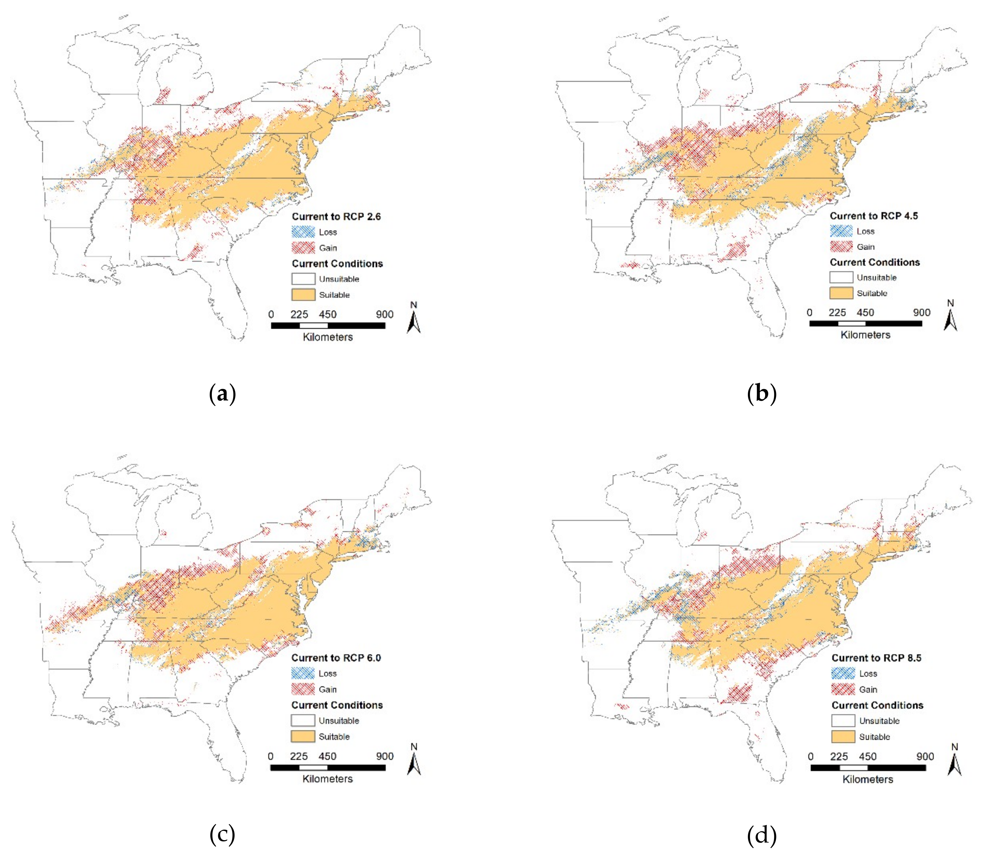
Under current conditions, our MaxEnt model predicted that T. c. carolina has a concentrated distribution within the middle of the eastern United States which is consistent with known range distributions. We expected that all future scenarios at a regional scale would result in the gain of suitable habitat and our results supported our hypothesis. We found that the proportion of suitable or unsuitable habitat showed moderate changes, i.e., 19% to 27%, it is critical to note, though, that where these changes occur will have large impacts on this species. Most of the changes, both gains and losses, occur on the distribution edge and relatively few changes within the center of the distribution. Although identifying these large-scale changes can help pinpoint critical priority areas for conservation efforts, we need finer-scale data to provide recommendations for on the ground management. In the future, suitable habitat may become inaccessible and isolated, therefore these models should distinguish between suitable and accessible locations [88]. Identifying these areas, requires downscaling from regional to local scale maps. Therefore, we compared local scale models across current and future scenarios. We found that suitable habitat decreases over time and is limited (i.e., ~15%). For our case study, percentage of forest was the driving factor for all models except Model 2 which suggests that the availability of shade will drive individual responses. Depending on which emission scenario is used will vary which quarter (i.e., wettest, driest, or warmest) will drive turtle responses. Once again highlighting the need for local scale climatic datasets, especially when modeling future suitable habitat. However, in all cases, suitable habitat is limited and fragmented, which makes dispersal challenging. Warming climate may make forest habitat more suitable; however, it will also make open areas less suitable and costly to cross. This suggests that canopy cover is important for dispersal, although NDVI is a good model for canopy cover, it cannot substitute for measuring canopy cover at a fine scale. Our results, though, support the need to incorporate land cover or other remote sensed data with climate factors, as percentage of habitat and NDVI contribute to habitat suitability. We recognize that projecting changes into the future is challenging and deriving models with more models requires a lot of assumptions. Therefore, a mixture of different techniques that address both changes in spatial and temporal scale are needed to tackle this challenge. From a climatic perspective, T. c. carolina may not need to move, especially at the northern part of the distribution, therefore other biological processes (i.e., increased disturbance, fragmentation, competition, predation) will drive local scale movements.
We examined this problem using both our CSMs and finer-scale environmental data in Oak Openings Region to evaluate whether individuals could feasibly disperse despite climatic changes. Based on field data an individual could feasibly disperse to a new area within its lifetime to accommodate a changing landscape. However, this assumes that there are relatively few to no barriers and constant movement each day towards potentially new suitable habitat, as well as an ability to detect these new habitats. For example, in Oak Openings Region, we found that individuals would need to travel a total of 22.95 to 23.84 km to get from one protected area to another (an additional 2 to 3 km from the straight-line distance) using only physical factors on the landscape. It would take individuals approximately 5.5 months to 9.5 years based on our minimum to maximum dispersal scenarios and seasonal activity period to travel this distance. Incorporating climate suitability produced a northern route and different scenarios did not vary much. We did find that the end portion of all models were the same and we suggest that local managers focus on protecting this route for potential dispersal. Although this distance ranges from 23% to 24% of the minimum dispersal distance scenario, it is unlikely that most of the individuals will take the least costly pathway, always following a straight-line path. Individuals would have to carefully traverse a multitude of suboptimal habitat including roads, rivers, crops, and developed areas. Additionally, individuals would have to traverse a variety of thermal gradients that may become too intolerable in the future. Individuals would be able to travel the required distance; however, when considering other structural features, many individuals would likely perish trying to disperse such large distances. T. c. carolina can persist in developed areas and can traverse croplands and flooded areas; however, they are susceptible to road mortality. Deaths on roads often change the population demographic and cause skewed adult sex ratios [89]. Additionally, this species is more susceptible to road mortality than other turtle species because they tend to close their shell when threatened and remain closed for longer periods of time [90]. Increased road traffic will increase the probability of mortality and assuming no further habitat changes, will lead to a threshold effect that causes widespread local extinction [91]. Although we found that there will be more suitable habitat in the future, it may not do any good with continued habitat fragmentation. We found that this species will face many difficult barriers and potentially have increased mortality when dispersing to future suitable habitat even with expanding suitable habitat, it may not be accessible.
Although T. c. carolina may not be as heavily impacted by climatic changes in terms of suitable area at the landscape-scale, it is important to provide a model for local scale context. T. c. carolina will remain under threat from a variety of sources, e.g., habitat destruction, invasive species, environmental pollution, disease, unsustainable use [5]. Therefore, models should incorporate other biologically relevant variables (e.g., roads, land cover, elevation, streams/lakes, etc.) to represent the synergistic effects of multiple threats. Such a multifaceted approach is critical because the response of local populations will be dependent on regional weather patterns and local structural characteristics. In addition, climate change interacts with the landscape by altering the configuration and composition of land cover. For an example, lakes are sensitive indicators of climate alterations such as fluctuating water levels [92] and timing changes in ice formation and thawing [93]. As with many other studies, land-use patterns are often a larger driving factor that influences populations more so than climate alone [94,95]. Our climatic habitat models illustrate that climatic change may be beneficial for this species; however, there are local scale challenges when other factors are examined that will affect how the species responds to these changes.

5. Conclusions

There is a critical need to protect and manage a flagship reptilian species such as T. c. carolina. We developed CSMs for this vulnerable species and evaluated the climatic variables that are influential in determining the geographic distribution and we predicted changes in potentially suitable habitat between different time periods. Our results predict moderate suitable habitat expansion. Additionally, we have identified areas that are susceptible to loss or gains in habitat within T. c. carolina distribution that can be monitored or managed. One of the most important aspects of our approach is to consider climate change impacts across a range of temporal and spatial scales from regional climate models to local occupancy models. Understanding the local context of large- scale changes is necessary to effectively manage for potential impacts on native flora and fauna and can highlight critical priorities. In addition to identifying where suitable habitat is and will be, we suggest that land managers should work towards increasing connectivity among suitable areas to facilitate dispersal. However, to examine these local scales, we need finer scale climatic data in combination with a variety of remotely sensed and locally collected data to inform our models. Finally, we suggest that future studies incorporate other dynamic ecological factors that influence distribution shifts.

Supplementary Materials

The following are available online at https://www.mdpi.com/2072-4292/12/5/836/s1, Table S1: The correlation matrix for nineteen bioclimatic variables, Figure S1: Response curves of the top two bioclimatic predictors based on the highest percent contribution for (a,b) current conditions; (c,d) 2050 RCP 2.6; (e,f) 2050 RCP 8.5., Figure S2: Alternative climatic suitability maps for T. c. carolina for four different time periods: (a) Last Glacial Maximum; (b) Current; (c) 2050 RCP 2.6; (d) 2050 RCP 4.5; (e) 2050 RCP 6.5; (f) 2050 RCP 8.5, Figure S3: Response curves of the top two environmental predictor variables based on the highest percent contribution for (a,b) current conditions; (c,d) 2050 RCP 2.6; (e,f) 2050 RCP 8.5.

Author Contributions

Conceptualization, A.K.M. and K.V.R.; Data curation, A.K.M.; Formal analysis, A.K.M.; Funding acquisition, A.K.M. and K.V.R.; Methodology, A.K.M.; Project administration, K.V.R.; Resources, K.V.R.; Supervision, K.V.R.; Writing—original draft preparation, A.K.M.; writing—review and editing, A.K.M. and K.V.R. All authors have read and agreed to the published version of the manuscript.

Funding

This research for the dispersal analyses was funded by Katzner Graduate Student Research and Professional Development, Barbara Long Masters Biological Sciences Research Award, Toledo Naturalists’ Association Mayfield Award, and Western New York Marv Aures/Bob Krantz Grant. All funding received was used for purchasing field supplies for radio telemetry study.

Acknowledgments

Thank you to numerous field assistants who assisted in the collection of occurrence data and to all the citizen scientists who contributed to the GBIF database. Thanks to the anonymous reviewers, committee members, and members of the Root lab for their support and feedback on early drafts. Thanks to the Bowling Green State University Biological Sciences department for supporting this research.

Conflicts of Interest

The authors declare no conflict of interest. The funders had no role in the design of the study; in the collection, analyses, or interpretation of data; in the writing of the manuscript, or in the decision to publish the results.

References

  1. Sala, O.; Chapin, F.S., III; Armesto, J.J.; Berlow, E.; Bloomfield, J.; Dirzo, R.; Huber-Sanwald, E.; Huenneke, L.F.; Jackson, R.B.; Kinzig, A.; et al. Global biodiversity scenarios for the year 2100. Science 2000, 287, 1770–1774. [Google Scholar] [CrossRef] [PubMed]
  2. Root, T.L.; Price, J.T.; Hall, K.R.; Schneider, S.H.; Rosenzweig, C.; Pounds, J.A. Fingerprints of global warming on wild animals and plants. Nature 2003, 421, 57–60. [Google Scholar] [CrossRef] [PubMed]
  3. Araujo, M.B.; Thuiller, W.; Pearson, R.G. Climate warming and the decline of amphibians and reptiles in Europe. J. Biogeogr. 2006, 33, 1712–1728. [Google Scholar] [CrossRef]
  4. Carey, C.; Alexander, M.A. Climate change and amphibian declines: Is there a link? Divers. Distrib. 2003, 9, 111–121. [Google Scholar] [CrossRef] [Green Version]
  5. Gibbons, J.W.; Scott, D.E.; Ryan, T.J.; Buhlmann, K.A.; Tuberville, T.D.; Metts, B.S.; Greene, J.L.; Mills, T.; Leiden, Y.; Poppy, S.; et al. The global decline of reptiles, déjà vu amphibians. BioScience 2000, 50, 653–666. [Google Scholar] [CrossRef] [Green Version]
  6. Sahlean, T.C.; Gherghel, I.; Papes, M.; Zamfirescus, R. Refining climate change projections for organisms with low dispersal abilities: A case study of the Caspian whip snake. PLoS ONE 2014, 9, e91994. [Google Scholar] [CrossRef] [PubMed]
  7. Wake, D.B. Climate change implicated in amphibian and lizard declines. Proc. Natl. Acad. Sci. USA 2007, 104, 8201–8202. [Google Scholar] [CrossRef] [Green Version]
  8. Parmesan, C. Ecological and evolutionary responses to recent climate change. Annu. Rev. Ecol. Evol. Syst. 2006, 37, 637–669. [Google Scholar] [CrossRef] [Green Version]
  9. Niehaus, A.C.; Angiletta, M.J.; Sears, M.W.; Franklin, C.E.; Wilson, R.S. Predicting the physiological performance of ectotherms in fluctuating thermal environments. J. Exp. Biol. 2012, 215, 694–701. [Google Scholar] [CrossRef] [Green Version]
  10. Huey, R.B.; Slatkin, M. Cost and benefits of lizard thermoregulation. Quart. Rev. Biol. 1976, 51, 363–384. [Google Scholar] [CrossRef]
  11. Huey, R.B. Physiological consequences of habitat selection. Am. Nat. 1991, 137, S91–S115. [Google Scholar] [CrossRef] [Green Version]
  12. Erskine, D.J.; Hutchison, V.H. Melatonin and behavioral thermoregulation in the turtle, Terrapene carolina triunguis. Physiol. Behav. 1981, 26, 991–994. [Google Scholar] [CrossRef]
  13. do Amaral, J.P.S.; Marvin, G.A.; Hutchinson, V.H. Thermoregulation in the box turtles Terrapene carolina and Terrapene ornata. Can. J. Zool. 2002, 80, 934–943. [Google Scholar] [CrossRef] [Green Version]
  14. do Amaral, J.P.S.; Marvin, G.A.; Hutchinson, V.H. The influence of bacterial lipopolysaccharide on the thermoregulation of the box turtle Terrapene carolina. Physiol. Biochem. Zool. 2002, 75, 273–282. [Google Scholar] [CrossRef]
  15. Roe, J.H.; Wild, K.H.; Hall, C.A. Thermal biology of eastern box turtles in a longleaf pine system managed with prescribed fire. J. Them. Biol. 2017, 69, 325–333. [Google Scholar] [CrossRef]
  16. Parlin, A.F.; do Amaral, J.P.S.; Dougherty, J.K.; Stevens, M.H.H.; Schaeffer, P.J. Thermoregulatory performance and habitat selection of the eastern box turtle (Terrapene carolina carolina). Conserv. Physiol. 2017, 5, cox070. [Google Scholar] [CrossRef] [Green Version]
  17. Sturbaum, B.A. Temperature regulation in turtles. Comp. Biochem. Phys. A. 1981, 72, 615–620. [Google Scholar] [CrossRef]
  18. Ziolkowska, E.; Ostapowicz, K.; Radeloff, V.C.; Kuemmerle, T.; Sergiel, A.; Zwijacz-Kozica, T.; Zieba, F.; Smietana, W.; Selva, N. Assessing differences in connectivity based on habitat versus movement models for brown bears in the Carpathians. Lands. Ecol. 2016, 31, 1863–1882. [Google Scholar] [CrossRef] [Green Version]
  19. Bradshaw, W.E.; Holzapfel, C.M. Evolutionary response to rapid climate change. Science 2006, 312, 1477–1478. [Google Scholar] [CrossRef] [Green Version]
  20. Hughes, L. Biological consequences of global warming: Is the signal already apparent? Trends Ecol. Evol. 2000, 15, 56–61. [Google Scholar] [CrossRef]
  21. Iverson, L.R.; Prasad, A.K.M. Predicting abundance of 80 tree species following climate change in the eastern United States. Ecol. Monogr. 1998, 68, 465–485. [Google Scholar] [CrossRef]
  22. Massot, M.; Clobert, J.; Ferriere, R. Climate warming, dispersal inhibition and extinction risk. Global Change Biol. 2008, 14, 461–469. [Google Scholar] [CrossRef]
  23. Matthews, S.; O’Connor, R.; Iverson, L.R.; Prasad, A.K.M. Atlas of climate change effects in 150 bird species of the eastern United States; Technical Report; NE-GTR-318; USDA Forest Service, 2004; p. 340. Available online: https://www.fs.fed.us/ne/newtown_square/publications/technical_reports/pdfs/2004/gtr318/ne_gtr318.pdf (accessed on 11 October 2019).
  24. McCarty, J.P. Ecological consequences of recent climate change. Conserv. Biol. 2002, 15, 320–331. [Google Scholar] [CrossRef]
  25. Root, T.L.; MacMynowski, D.P.; Mastrandrea, M.D.; Schneider, S.H. Human-modified temperatures induce species changes: Joint attribution. Proc. Natl. Acad. Sci. USA 2005, 102, 7465–7469. [Google Scholar] [CrossRef] [PubMed] [Green Version]
  26. Skelly, D.K.; Joseph, L.N.; Possingham, H.P.; Freidenburg, L.K.; Farrugia, T.J.; Kinnison, M.T.; Hendry, A.P. Evolutionary responses to climate change. Conserv. Biol. 2007, 21, 1353–1355. [Google Scholar] [CrossRef] [PubMed]
  27. Thomas, C.D.; Cameron, A.; Green, R.E.; Bakkenes, M.; Beaumont, L.J.; Collingham, Y.C.; Erasmus, B.F.N.; Ferreira de Siqueira, M.; Grainger, A.; Hannah, L.; et al. Extinction risk from climate change. Nature 2004, 427, 145–148. [Google Scholar] [CrossRef] [PubMed]
  28. Walther, G.R.; Post, E.; Convey, P.; Mensel, A.; Parmesan, C.; Beebee, T.J.C.; Fomentin, J.; Hoegh-Guldberg, O.; Bairlein, F. Ecological responses to recent climate change. Nature 2002, 416, 389–395. [Google Scholar] [CrossRef]
  29. Pearson, R.G.; Dawson, T.P. Predicting the impacts of climate change on the distribution of species: Are bioclimate envelope models useful? Glob. Ecol. Biogeogr. 2003, 12, 361–371. [Google Scholar] [CrossRef] [Green Version]
  30. Araújo, M.B.; Pearson, R.G.; Thuiller, W.; Erhard, M. Validation of species-climate impact models under climate change. Glob. Change Biol. 2005, 11, 1504–1513. [Google Scholar] [CrossRef] [Green Version]
  31. Bombi, P.; Salvi, D.; Vignoli, L.; Bologna, M.A. Modelling Bedriaga’s rock lizard distribution in Sardinia: An ensemble approach. Amphibia-Reptilia 2009, 30, 413–424. [Google Scholar] [CrossRef] [Green Version]
  32. Cowling, S.A.; Maslin, M.A.; Sykes, M.T. Paleovegetation simulations of lowland Amazonia and implications for neotropical allopatry and speciation. Quat. Res. 2001, 55, 140–149. [Google Scholar] [CrossRef]
  33. DeMatteo, K.E.; Loiselle, B.A. New data on the status and distribution of the bush dog (Speothos venaticus): Evaluating its quality of protection and directing research efforts. Biol. Conserv. 2008, 141, 2494–2505. [Google Scholar] [CrossRef]
  34. Doko, T.; Fukui, H.; Kooiman, A.; Toxopeus, A.G.; Ichinose, T.; Chen, W.; Skidmore, A.K. Identifying habitat patches and potential ecological corridors for remnant Asiatic black bear (Ursus thibetanus japonicus) populations in Japan. Ecol. Model. 2011, 222, 748–761. [Google Scholar] [CrossRef]
  35. Dormann, C.F.; McPherson, J.M.; Araujo, M.B.; Bivand, R.; Bolliger, J.; Carl, G.; Davies, R.G.; Hirzel, A.; Jetz, W.; Kissling, W.D.; et al. Methods to account for spatial autocorrelation in the analysis of species distributional data: A review. Ecography 2007, 30, 609–628. [Google Scholar] [CrossRef] [Green Version]
  36. Iverson, L.R.; Prasad, A.; Schwartz, M.W. Modeling potential future individual tree-species distributions in the eastern United States under a climate change scenario: A case study with Pinus virginiana. Ecol. Model. 1999, 115, 77–93. [Google Scholar] [CrossRef]
  37. Lee, D.N.; Papes, M.; Van Den Bussche, R.A. Present and potential future distribution of common vampire bats in the Americas and the associated risk to cattle. PLoS ONE 2012, 7, e42466. [Google Scholar] [CrossRef] [Green Version]
  38. Moussalli, A.; Moritz, C.; Williams, S.E.; Carnaval, A.C. Variable responses of skinks to a common history of rainforest fluctuation: Concordance between phylogeography and palaeo-distribution models. Mol. Ecol. 2009, 18, 483–499. [Google Scholar] [CrossRef]
  39. Owens, H.L.; Bentley, A.C.; Peterson, A.T. Predicting suitable environments and potential occurrences for coelacanths (Latimeria spp.). Biodivers. Conserv. 2012, 21, 577–587. [Google Scholar] [CrossRef]
  40. Papeş, M.; Gaubert, P. Modelling ecological niches from low numbers of occurrences: Assessment of the conservation status of poorly known viverrids (Mammalia, carnivora) across two continents. Divers. Distrib. 2007, 13, 890–902. [Google Scholar] [CrossRef]
  41. Peterson, A.T. Predicting species’ geographic distributions based on ecological niche modeling. Condor 2001, 103, 599–605. [Google Scholar] [CrossRef]
  42. Peterson, A.T.; Papeş, M.; Kluza, D.A. Predicting the potential invasive distributions of four alien plant species in North America. Weed Sci. 2003, 51, 863–868. [Google Scholar] [CrossRef]
  43. Puschendorf, R.; Carnaval, A.C.; VanDerWal, J.; Zumbado-Ulate, H.; Chaves, G.; Bolanos, F.; Alford, R.A. Distribution models for the amphibian chytrid Batrachochytrium dendrobatidis in Costa Rica: Proposing climatic refuges as a conservation tool. Divers. Distrib. 2009, 15, 401–408. [Google Scholar] [CrossRef]
  44. Raxworthy, C.J.; Ingram, C.M.; Rabibisoa, N.; Pearson, R.G. Applications of ecological niche modeling for species delimitation: A review and empirical evaluation using day geckos (Phelsuma) from Madagascar. Syst. Biol. 2007, 56, 907–923. [Google Scholar] [CrossRef] [PubMed] [Green Version]
  45. Schwartz, M.W.; Iverson, L.R.; Prasad, A.K.M.; Matthews, S.N.; O’Connor, R.J. Predicting extinctions as a result of climate change. Ecology 2006, 87, 1611–1615. [Google Scholar] [CrossRef]
  46. Wiens, J.J. What is speciation and how should we study it? Am. Nat. 2004, 163, 914–923. [Google Scholar] [CrossRef] [Green Version]
  47. Wiens, J.J. The causes of species richness patterns across space, time, and clades and the role of “ecological limits”. Q. Rev. Biol. 2011, 86, 75–96. [Google Scholar] [CrossRef] [PubMed] [Green Version]
  48. Wilson, J.J.; Lantz, V.A.; MacLean, D.A. A benefit-cost analysis of establishing protected natural areas in New Brunswick, Canada. Forest Policy Econ. 2010, 12, 94–103. [Google Scholar] [CrossRef]
  49. Beaumont, L.J.; Hughes, L.; Pitman, A.J. Why is the choice of future climate scenarios for species distribution modelling important? Ecol. Lett. 2008, 11, 1135–1146. [Google Scholar] [CrossRef]
  50. Pearson, R.G.; Thuiller, W.; Araujo, M.B.; Martinez-Meyer, E.; Brotons, L.; McClean, C.; Miles, L.; Segurado, P.; Dawson, T.P.; Lees, D.C. Model-based uncertainty in species range prediction. J. Biogeogr. 2006, 33, 1704–1711. [Google Scholar] [CrossRef]
  51. Seo, C.; Thorne, J.H.; Hannah, L.; Thuiller, W. Scale effects in species distribution models: Implications for conservation planning under climate change. Biol. Lett. 2009, 5, 39–43. [Google Scholar] [CrossRef] [Green Version]
  52. Thuiller, W. Patterns and uncertainties of species’ range shifts under climate change. Glob. Change Biol. 2004, 10, 2020–2027. [Google Scholar] [CrossRef]
  53. Araújo, M.B.; New, M. Ensemble forecasting of species distributions. Trends Ecol. Evol. 2007, 22, 42–47. [Google Scholar] [CrossRef] [PubMed]
  54. Elith, J.; Graham, C.H.; Anderson, R.P.; Dudik, M.; Ferrier, S.; Guisan, A.; Hijmans, R.J.; Huettmann, F.; Leathwick, J.R.; Lehman, A.; et al. Novel methods improve prediction of species’ distributions from occurrence data. Ecography 2006, 29, 129–151. [Google Scholar] [CrossRef] [Green Version]
  55. Hijmans, R.J.; Cameron, S.E.; Parra, J.L.; Jones, P.G.; Jarvis, A. Very high resolution interpolated climate surfaces for global land areas. Int. J. Climatol. 2005, 25, 1965–1978. [Google Scholar] [CrossRef]
  56. Tavernia, B.G.; Nelson, M.D.; Goerndt, M.E.; Walters, B.F.; Toney, C. Changes in forest habitat classes under alternative climate and land-use change scenarios in the northeast and Midwest, USA. Math. Comput. Forest. Nat. Resour. Sci. 2013, 5, 135–150. [Google Scholar]
  57. Yousefkhani, S.S.H.; Aliabadian, M.; Rastegar-Pouyani; Darvish, J. Predicting the impact of climate change on the distribution pattern of Agamura persica (Dumeril, 1856) (SquamataL Gekkonidae) in Iran. Belgian J. Zool. 2017, 2, 137–142. [Google Scholar] [CrossRef]
  58. Xu, X.; Zhang, H.; Yue, J.; Xie, T.; Xu, Y.; Tian, Y. Predicting shifts in the suitable climatic distribution of walnut (Juglans regia L.) in China: Maximum entropy model paves the way to forest management. Forests 2018, 9, 303. [Google Scholar] [CrossRef] [Green Version]
  59. Elith, J.; Phillips, S.J.; Hastie, T.; Dudik, M.; Chee, T.E.; Yates, C.J. A statistical explanation of MaxEnt for ecologists. Divers. Distrib. 2011, 17, 43–57. [Google Scholar] [CrossRef]
  60. Phillips, S.J.; Dudik, M.; Schapire, R.E. A maximum entropy approach to species distribution modeling. In Proceedings of the Twenty-First International Conference on Machine Learning, Banff, AB, Canada, 4–8 July 2004; pp. 655–662. [Google Scholar] [CrossRef] [Green Version]
  61. Global Biodiversity Information Facility. Available online: https://www.gbif.org/ (accessed on 30 April 2019).
  62. Martin, A.K.M.; Root, K.V. A multi-scale spatial analysis of eastern box turtle movements within Oak Openings Region. Unpublished work.
  63. Karger, D.N.; Conrad, O.; Böhner, J.; Kawohl, T.; Kreft, H.; Soria-Auza, R.W.; Zimmermann, N.E.; Linder, H.P.; Kessler, M. Climatologies at high resolution for the earth’s land surface areas. Sci. Data 2017, 4, 170122. [Google Scholar] [CrossRef] [Green Version]
  64. Karger, D.N.; Conrad, O.; Böhner, J.; Kawohl, T.; Kreft, H.; Soria-Auza, R.W.; Zimmermann, N.E.; Linder, H.P.; Kessler, M. Data from: Climatologies at high resolution for the earth’s land surface areas. Dryad Digital Repository 2017. [Google Scholar] [CrossRef]
  65. ESRI. ArcCatalog Version 10.2.2; Environmental Systems Research Institute, Inc. (ESRI): Redlands, CA, USA, 2016. [Google Scholar]
  66. ESRI. ArcGIS Version 10.2.2; Environmental Systems Research Institute, Inc. (ESRI): Redlands, CA, USA, 2016. [Google Scholar]
  67. Phillips, S.J. A brief tutorial on Maxent. Available online: http://biodiversityinformatics.amnh.org/open_source/maxent/ (accessed on 16 November 2019).
  68. United States Geological Survey. EarthExplorer. Available online: https://earthexplorer.usgs.gov/ (accessed on 15 December 2019).
  69. ENVI Development Team. ENVI Version 5.5; Harris Geospatial Solutions: Broomfield, CO, USA, 2018. [Google Scholar]
  70. United States Department of Agriculture Farm Service Agency. Common Land Units. Available online: https://datagateway.nrcs.usda.gov/ (accessed on 3 April 2017).
  71. McGarigal, K.; Marks, B.J. FRAGSTATS: Spatial Pattern Analysis Program for Quantifying Landscape Structure; Gen tech rep pnw-gtr-351; United States Department of Agriculture, Forest Service, Pacific Northwest Research Station: Corvaliis, OR, USA, 1995. [Google Scholar]
  72. U.S. Census Bureau. 2009 TIGER/Line Shapefiles; U.S. Census Bureau: Washington, DC, USA, 2009. [Google Scholar]
  73. USGS EarthExplorer. Available online: https://earthexplorer.usgs.gov/ (accessed on 7 November 2019).
  74. Root, K.V.; Martin, A.K. Oak Openings Region Biodiversity Model Final Report (Phase II); Technical Report; The Nature Conservancy Grant #10009843 2018. Available online: http://karenroot.net/documents/Oak_Openings_Model_Report_Phase_II.pdf (accessed on 7 November 2019).
  75. Case, M.J.; Stinson, K.A. Climate change impacts on the distribution of the allergenic plant, common ragweed (Ambrosia artemisiifolia) in the eastern United States. PLoS ONE 2018, 13, e0205677. [Google Scholar] [CrossRef] [PubMed]
  76. Lemoine, N.P. Climate change may alter breeding ground distributions of Eastern migratory monarchs (Danaus plexippus) via range expansion of Asclepias host plants. PLoS ONE 2015, 10, e0118614. [Google Scholar] [CrossRef] [PubMed] [Green Version]
  77. Pandey, R.; Papeş, M. Changes in future potential distributions of apex predator and mesopredator mammals in North America. Reg. Environ. 2018, 18, 1223–1233. [Google Scholar] [CrossRef]
  78. Kearney, M.; Shine, R.; Porter, W.P. The potential for behavioral thermoregulation to buffer ‘cold blooded’ animals against climate warming. Proc. Natl. Acad Sci. USA 2009, 106, 3835–3840. [Google Scholar] [CrossRef] [PubMed] [Green Version]
  79. Chen, J.; Saunders, S.C.; Crow, T.R.; Naiman, R.J.; Brosofske, K.D.; Mroz, G.D.; Brookshire, B.L.; Franklin, J.F. Microclimate in forest ecosystem and landscape ecology. Bioscience 1999, 49, 288–297. [Google Scholar] [CrossRef] [Green Version]
  80. Stefanescu, C.; Carnicer, J.; Penuelas, J. Determinants of species richness in generalist and specialist Mediterranean butterflies: The negative synergistic forces of climate and habitat change. Ecography 2011, 34, 353–363. [Google Scholar] [CrossRef]
  81. Popescu, V.D.; Rozylowicz, L.; Cogălniceanu, D.; Niculae, I.M.; Cucu, A.L. Moving into protected areas? Setting conservation priorities for Romanian reptiles and amphibians at risk from climate change. PLoS ONE 2013, 8, e79330. [Google Scholar] [CrossRef]
  82. Dore, M.H.I. Climate change and changes in global precipitation patterns: What do we know? Envriron. Int. 2005, 31, 1167–1181. [Google Scholar] [CrossRef]
  83. Yarnal, B.; Johnson, D.L.; Frakes, B.J.; Bowles, G.I.; Pascale, P. The flood of ’96 and its socioeconomic impacts in the Susquehanna River basin. J. Am. Water Resour. Assoc. 1997, 33, 1299–1312. [Google Scholar] [CrossRef]
  84. Frederickson, T.S. Thermal regulation and habitat use of the eastern box turtle in southwestern Virginia. Northeast. Nat. 2014, 21, 554–564. [Google Scholar] [CrossRef]
  85. Donaldson, B.M.; Echternacht, A.C. Aquatic habitat use relative to home range and seasonal movement of eastern box turtles (Terrapene carolina carolina: Emydidae) in eastern Tennessee. J. Herpetol. 2005, 39, 284–287. [Google Scholar] [CrossRef]
  86. Nasrabadi, R.; Rastegar-Pouyani, N.; Pouyani, E.R.; Kami, H.G.; Gharzi, A.; Yousefkhani, S.H. The effects of climate change on the distribution of European glass lizard Pseudopus apodus (PALLAS, 1775) in Eurasia. Ecol. Res. 2018, 33, 199–204. [Google Scholar] [CrossRef]
  87. Terribile, L.C.; Feitosa, D.T.; Pires, M.G.; de Almeida, P.C.R.; de Oliveira, G.; Diniz-Filho, J.A.F.; da Silva, J., Jr. Reducing Wallacean shortfalls for the coralsnakes of the Micrurus lemniscatus species complex: Present and future distributions under a changing climate. PLoS ONE 2018, 13, e0205164. [Google Scholar] [CrossRef] [PubMed]
  88. Miller, J.A.; Holloway, P. Incorporating movement in species distribution models. Prog. Phys. Geog. 2015, 39, 837–849. [Google Scholar] [CrossRef]
  89. Gibbs, J.P.; Steen, D.A. Trends in sex ratios of turtles in the United States: Implications of road mortality. Conserv. Biol. 2008, 19, 552–556. [Google Scholar] [CrossRef]
  90. Gooley, A.C. Testing the Behavioral Responses of West Virginia Turtles to Roads and Vehicles. Master’s Thesis, Marshall University, Huntington, WV, USA, 2010; p. 54. [Google Scholar]
  91. Kiester, A.R.; Willey, L.L. Terrapene carolina (Linnaeus 1758)-eastern box turtle, common box turtle. Chelonian Res. Monogr. 2015, 5, 085.1–085.25. [Google Scholar] [CrossRef] [Green Version]
  92. Williamson, C.E.; Saros, J.E.; Schindler, D.W. Climate change, Sentinels of Change. Science 2009, 323, 887–888. [Google Scholar] [CrossRef]
  93. Magnuson, J.J.; Robertson, D.M.; Benson, B.J.; Wynne, R.H.; Livingstone, D.M.; Arai, T.; Assel, R.A.; Barry, R.G.; Card, V.V.; Kuusisto, E.; et al. Historical trends in lake and river ice cover in the northern hemisphere. Science 2000, 289, 1743–1746. [Google Scholar] [CrossRef] [Green Version]
  94. Hof, C.; Levinsky, I.; Araujo, M.B.; Rahbeck, C. Rethinking species’ ability to cope with rapid climate change. Glob. Change Biol. 2011, 17, 2987–2990. [Google Scholar] [CrossRef]
  95. Rowe, R. Legacies of land use and recent climatic change: The small mammal fauna in the mountains of Utah. Am. Nat. 2007, 170, 242–257. [Google Scholar] [CrossRef]
Figure 1. Climatic habitat suitability continuous probability maps for T. c. carolina for four different time periods: (a) Last Glacial Maximum (LGM); (b) Current; (c) 2050 Representative Concentration Pathway (RCP) 2.6; (d) 2050 RCP 4.5; (e) 2050 RCP 6.0; (f) 2050 RCP 8.5. Color changes indicate probability of suitability, with blue indicating low to no probability and red indicating high probability.
Remotesensing 12 00836 g001
Figure 2. Predicted current (unsuitable and suitable) combined with future loss (in blue) and gain (in red) habitat for T. c. carolina. Future predictions are based on four emission scenarios for 2050 with changes from current to (a) 2050 Representative Concentration Pathway (RCP) 2.6; (b) 2050 RCP 4.5; (c) 2050 RCP 6.0; (d) 2050 RCP 8.5.
Remotesensing 12 00836 g002
Figure 3. Climatic habitat suitability maps for T. c. carolina for five models, which include six bioclimatic variables, percentage of forest, percentage of early successional, and normalized difference vegetation index (NDVI): (a) Model 1: Current; (b) Model 2: 2050 Representative Concentration Pathway (RCP) 2.6; (c) Model 3: 2050 RCP 4.5; (d) Model 4: 2050 RCP 6.0; and (e) Model 5: 2050 RCP 8.5 for Oak Openings Region in northwestern Ohio.
Remotesensing 12 00836 g003
Figure 4. The least cost paths that individuals can take from Oak Openings Preserve to Wildwood Metroparks for five scenarios. Model 1: Current, Model 2: 2050 Representative Concentration Pathway (RCP) 2.6, Model 3: 2050 RCP 4.5, Model 4: 2050 RCP 6.0, and Model 5: 2050 RCP 8.5. Least cost paths (colored lines) are overlaid on the cost layer with high travel cost (in red) and low travel cost (in blue) for current conditions.
Remotesensing 12 00836 g004
Table 1. The correlation matrix for six selected bioclimatic variables which includes average temperature (°C) and precipitation (mm) for wettest, driest, and warmest quarters. Abbreviations are: Temperature (T), Wettest (Wet), Driest (Dry), Warmest (Warm), Quarter (Q), and Precipitation (P).
LayerT of WetT of DryT of WarmP of WetP of DryP of Warm
T of Wet1.00−0.060.220.12−0.220.46
T of Dry−0.061.000.780.670.650.29
T of Warm0.220.781.000.620.380.33
P of Wet0.120.670.621.000.440.78
P of Dry−0.220.650.380.441.000.18
P of Warm0.460.290.330.780.181.00
Table 2. The bioclimatic profile which includes minimum, maximum, and mean of the selected bioclimatic factors for T. c. carolina occurrence data.
VariableMinimumMaximumMean
Mean Temperature of wettest quarter (°C)1.227.220.3
Mean Temperature of driest quarter (°C)−4.027.78.28
Mean temperature of warmest quarter (°C)17.427.724.4
Precipitation of wettest quarter (mm/quarter)221731351
Precipitation of driest quarter (mm/quarter)121448227
Precipitation of warmest quarter (mm/quarter)201569324
Table 3. The maximum test sensitivity plus specificity threshold (MSS) and model area under the curve (AUC) values with standard deviation for the Last Glacial Maximum (LGM), Current conditions, and four future Representative Concentration Pathway (RCP) scenarios. Including the percentage of suitable and unsuitable habitat based on the MSS threshold.
ScenarioMSSAUC ValuesSuitable Habitat (%)Unsuitable Habitat (%)
LGM0.31960.823 ± 0.00430.3%69.7%
Current0.35980.819 ± 0.00524.5%75.5%
RCP 2.60.31090.815 ± 0.00429.1%70.9%
RCP 4.50.35840.811 ± 0.00628.9%71.1%
RCP 6.00.32600.808 ± 0.00529.2%70.8%
RCP 8.50.32610.810 ± 0.00228.2%71.8%
Table 4. For each climate scenario model is presented the percent contribution (% C) and permutation importance (PI) for each environmental predictor variable with the highest contribution in bold. All temperature variables are in (°C) and all precipitation variables are in (mm). Abbreviations are: Temperature (T), Wettest (Wet), Driest (Dry), Warmest (Warm), Quarter (Q), and Precipitation (P).
LGM CurrentRCP 2.6RCP 4.5RCP 6.0RCP 8.5
Variable% CPI% CPI% CPI% CPI% CPI% CPI
Mean T of Wet Q 3.04.015.26.923.423.714.411.419.27.821.712.4
Mean T of Dry Q 45.123.731.330.120.324.233.728.825.527.730.235.0
Mean T of Warm Q35.641.630.425.227.823.727.423.328.923.725.321.5
P of Wet Q1.86.42.29.42.110.41.76.91.96.72.26.4
P of Dry Q12.517.219.925.623.327.518.525.823.832.614.921.5
P of Warm Q2.06.41.02.83.14.14.43.90.61.55.73.3
Table 5. Predicted changes in the climatically suitable habitat area of T. c. carolina under varying climate scenarios within their distribution range. Abbreviations: Last Glacial Maximum (LGM) and Representative Concentration Pathway (RCP).
Change ScenarioUnchangedGainLossTotal change (= Gain − Loss) 1
LGM -> Current45%13%42%−29%
Current -> 2050 RCP 2.654%37%10%27%
Current -> 2050 RCP 4.545%39%16%23%
Current -> 2050 RCP 6.050%38%12%26%
Current -> 2050 RCP 8.547%36%17%19%
1 A positive value indicates expansion of suitable habitat.
Table 6. Predicted changes in the percent of climatically suitable habitat for T. c. carolina using hotspot maps based on the number of environmental predictor layers that overlap with one another. We classified low overlap (0–2 layers), medium overlap (3–4), and high overlap (5–6). Abbreviations: Last Glacial Maximum (LGM) and Representative Concentration Pathway (RCP).
# of Layer OverlapLGMCurrentRCP 2.6RCP 4.5RCP 6.0RCP 8.5
Low0.0%0.0%0.5%0.3%0.2%0.3%
Medium49.4%45.1%54.9%71.7%72.3%76.5%
High50.6%54.9%44.6%28.0%27.5%23.2%
Table 7. The maximum test sensitivity plus specificity threshold (MSS) and model area under the curve (AUC) values with standard deviation for Current conditions and four future Representative Concentration Pathway (RCP) scenarios. Including the percentage of suitable and unsuitable habitat based on the MSS threshold.
Model #ScenarioMSSAUC ValuesSuitable Habitat (%)Unsuitable Habitat (%)
1Current0.34520.852 ± 0.07622.0%78.0%
2RCP 2.60.40030.905 ± 0.03914.8%85.2%
3RCP 4.50.40420.896 ± 0.003914.4%85.6%
4RCP 6.00.42770.883 ± 0.06313.9%86.1%
5RCP 8.50.31940.860 ± 0.07018.1%81.9%
Table 8. Presented are the percent contribution (% C) and permutation importance (PI) for each environmental predictor variable with the highest contribution in bold for each Model. All temperature variables are in (°C) and all precipitation variables are in (mm). Abbreviations are: Mean Temperature (MT), Wettest (Wet), Driest (Dry), Warmest (Warm), Quarter (Q), Percentage (%) Precipitation (P), Early successional (ES), and Land surface temperature (LST).
Model 1Model 2Model 3Model 4Model 5
Variables% CPI% CPI% CPI% CPI% CPI
MT of Wet Q 5.317.312.17.75.63.110.83.722.432.2
MT of Dry Q 1.12.14.94.524.146.712.923.821.414.9
MT of Warm Q1.00.046.664.710.6950.30.517.936.3
P of Wet Q11.555.30.40.62.70.33.812.40.00.0
P of Dry Q18.20.011.010.36.115.83.812.43.14.6
P of Warm Q5.111.80.41.51.20.80.00.04.25.4
% of forest45.79.018.25.541.317.837.111.227.74.0
% of ES6.34.52.42.05.34.34.13.11.80.3
NDVI5.70.03.93.23.11.86.46.21.42.4

