Use of SAR and Optical Time Series for Tropical Forest Disturbance Mapping

Abstract

Frequent cloud cover and fast regrowth often hamper topical forest disturbance monitoring with optical data. This study aims at overcoming these limitations by combining dense time series of optical (Sentinel-2 and Landsat 8) and SAR data (Sentinel-1) for forest disturbance mapping at test sites in Peru and Gabon. We compare the accuracies of the individual disturbance maps from optical and SAR time series with the accuracies of the combined map. We further evaluate the detection accuracies by disturbance patch size and by an area-based sampling approach. The results show that the individual optical and SAR based forest disturbance detections are highly complementary, and their combination improves all accuracy measures. The overall accuracies increase by about 3% in both areas, producer accuracies of the disturbed forest class increase by up to 25% in Peru when compared to only using one sensor type. The assessment by disturbance patch size shows that the amount of detections of very small disturbances (< 0.2 ha) can almost be doubled by using both data sets: for Gabon 30% as compared to 15.7–17.5%, for Peru 80% as compared to 48.6–65.7%.

1. Introduction

The mapping of forest disturbances is an important component in sustainable forest management and in implementing climate policy initiatives, such as the UN’s Reducing Emissions from Deforestation and Forest Degradation (REDD+) programme. In this paper, we use the term forest disturbance as an umbrella term for all forest changes that result from both deforestation and from forest degradation. According to both FAO and UNFCCC, deforestation is a conversion from forest land to non-forest land. Since, in many cases, we do not know the future fate of the disturbance patches, we cannot further classify them. Instead, the analysis of this study puts a focus on the size of the detected disturbance patches. Today, remote sensing applications are widely used to monitor tropical forests and their changes at large spatial scales. Most tropical forest monitoring systems are based on optical data sets and focus on large-deforestation areas, for which user accuracies around 90% and producer accuracies above 75% are reported [1,2,3]. In addition, recent developments have led to automated forest monitoring systems that are based on medium to high spatial resolution Earth Observation (EO) data and allow tracking forest changes in near real-time (NRT), such as Global Forest Watch Alerts for the humid tropical forests [4] and the DETER system in Brazil [5]. While methods for large area deforestation monitoring have improved considerably over the last years, there still is a lack of methods that accurately detect forest degradation and small forest changes. Forest degradation is thought to be a major source of carbon emissions [6], and thus needs to be better understood and integrated in REDD+ Monitoring & Measurement, Reporting and Verification (MRV) systems. A key driver of forest degradation is timber extraction by selective logging, where only a small subset of trees is harvested. The intensity of selective logging varies, depending on the amount of wood that is harvested, but usually the individual patches of change are small. Other less prominent drivers of forest degradation in developing countries include fuelwood collection and charcoal production, uncontrolled fire, and livestock grazing [7]. To accurately detect small patches of forest disturbance from selective logging and other degradation drivers, EO data of both high spatial and temporal resolution is required because gaps left by e.g., individual tree extraction are very small and quickly overgrow in tropical climates. EO data that have the potential to map forest degradation are now available: the Sentinel missions provide data at 10 m spatial resolution both in the optical and Synthetic Aperture Radar (SAR) domain and data are provided every five to 12 days.

Apart from rapid forest regrowth, tropical forest disturbance mapping with optical data is also limited by the number of available cloud-free observations. C-band SAR data from the Sentinel-1 mission (central frequency of 5.404 GHz) can be acquired independent of weather conditions and daytime, leading to very dense time series of EO data. The two-satellite constellation of Sentinel-1 has a potential six-day exact repeat cycle, but the tropical regions are only covered by one satellite, leading to a 12-day repeat cycle. Some tropical areas are only covered by one descending or one ascending orbit. Information on revisit frequency and the available pass directions can be obtained from the Sentinel-1 observation scenario from ESA (https://sentinel.esa.int/web/sentinel/missions/sentinel-1/observation-scenario). By combining the vast amounts of new EO data from the Sentinel-1 (S-1), Sentinel-2 (S-2), and Landsat 8 (L8) missions, it is possible to strongly increase the temporal density of available EO data and additionally exploit multi-sensor information for forest monitoring. The Sentinel-2 constellation and Landsat 8 have repeat cycles of five days and 16 days, respectively. Together, these two missions provide up to eight images per month for tropical regions and strongly increase the temporal density of image time series. However, the number of usable cloud-free observations is site specific as it strongly depends on regional cloud cover. An assessment of available Landsat 7 and 8 images for Peru showed that, on average, less than 50% of all potential observations are cloud-free observations and cloud cover has significant intra-annual and regional variation [8]. The combination of all available cloud-free optical observations and SAR data allows to develop near real-time forest disturbance mapping systems at high spatial resolution, which can be used to more accurately detect small scale forest disturbances.

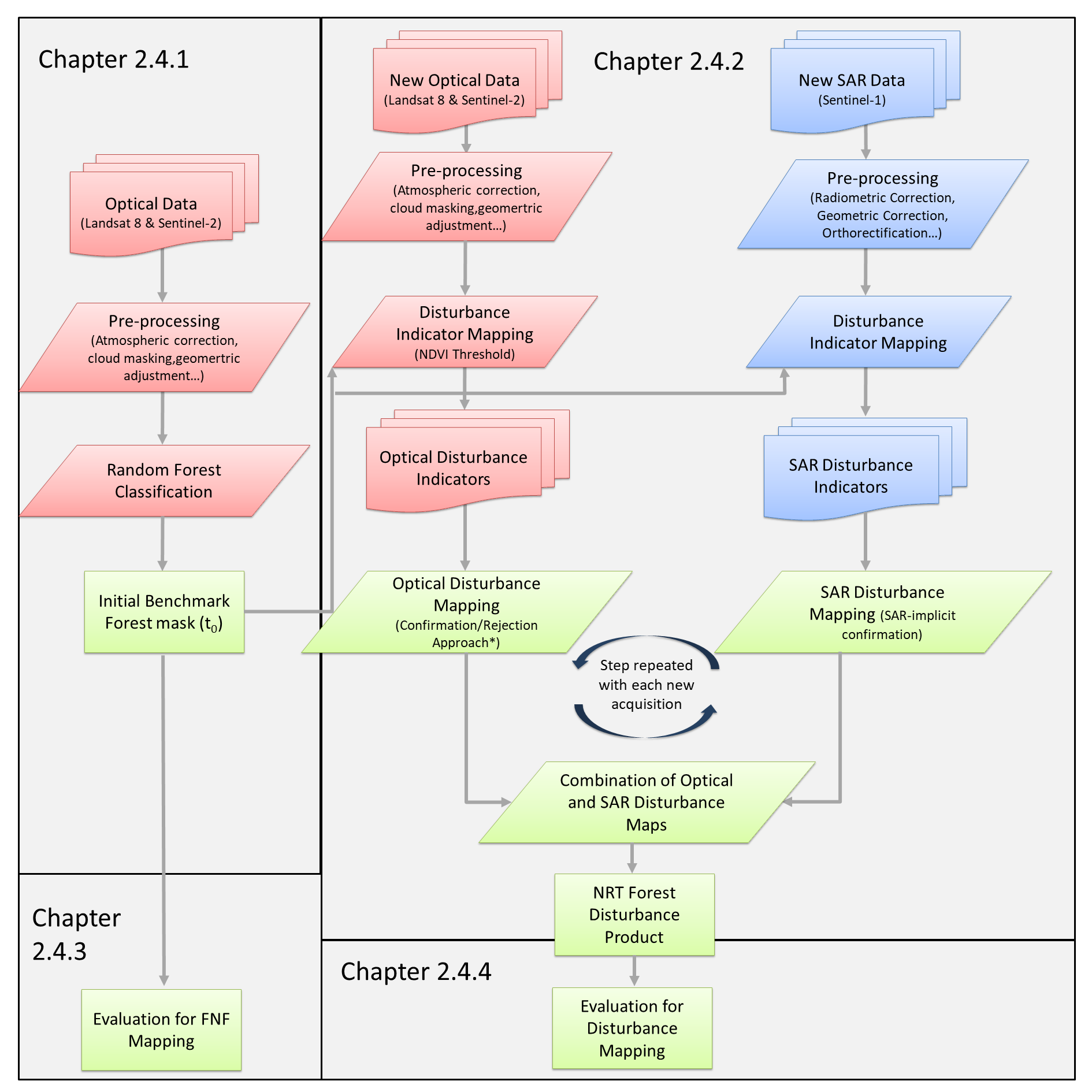
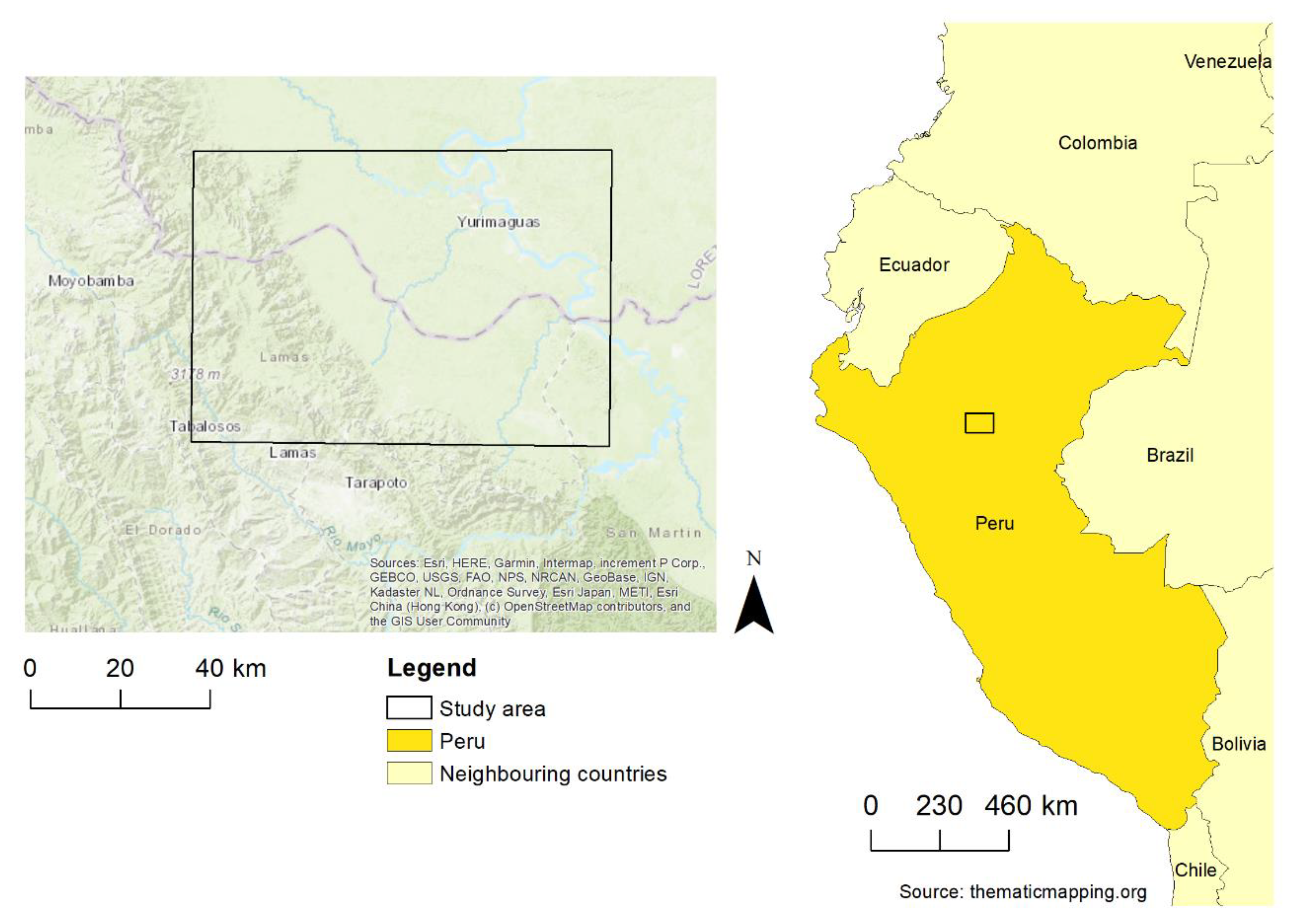
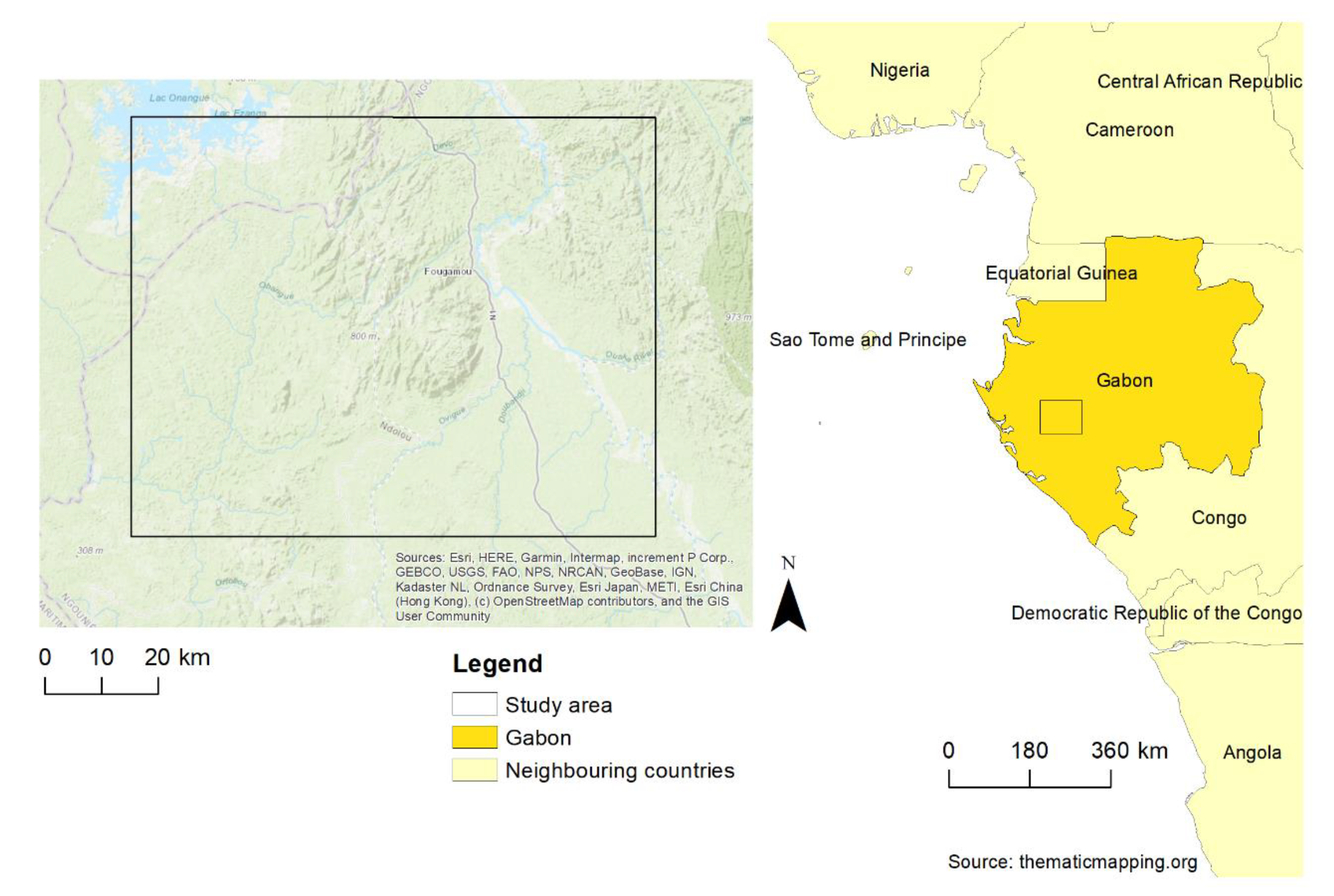
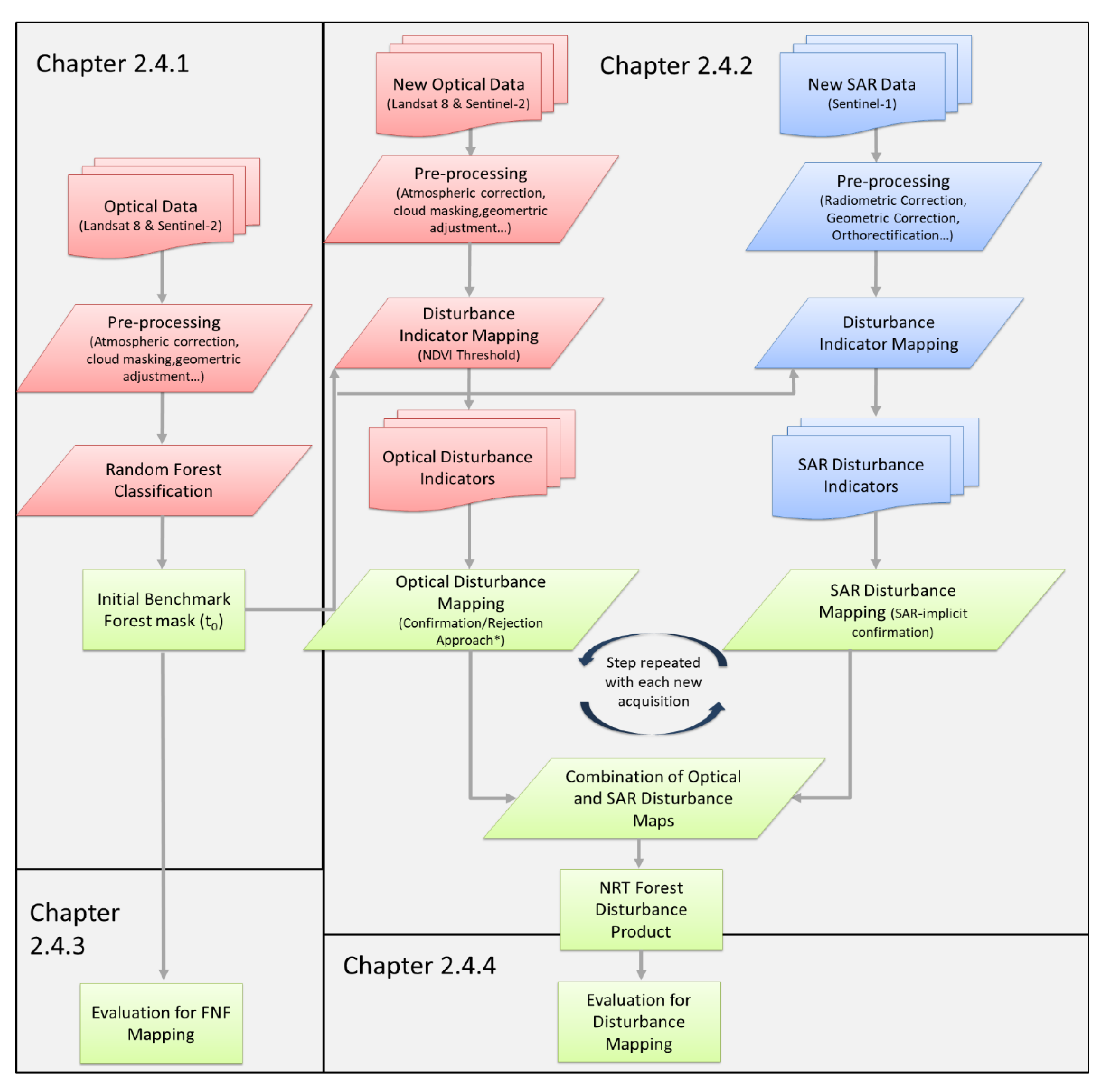
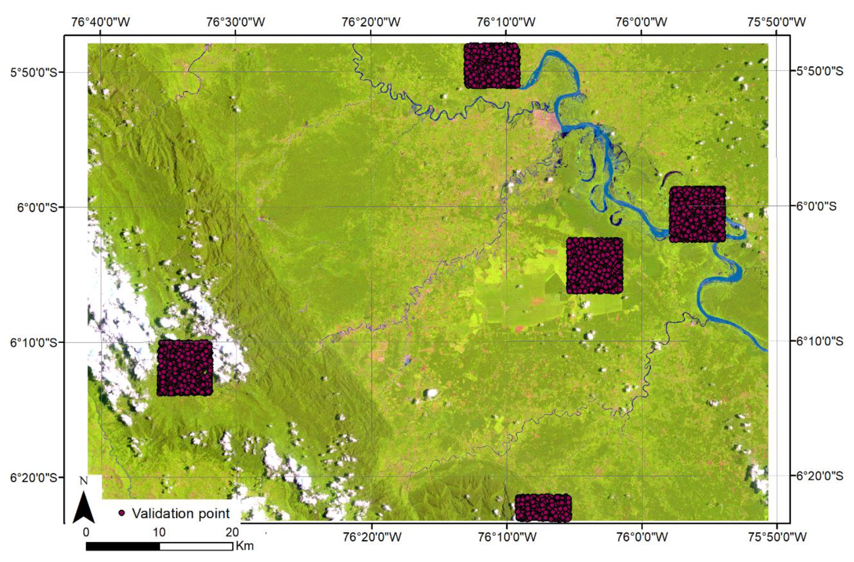
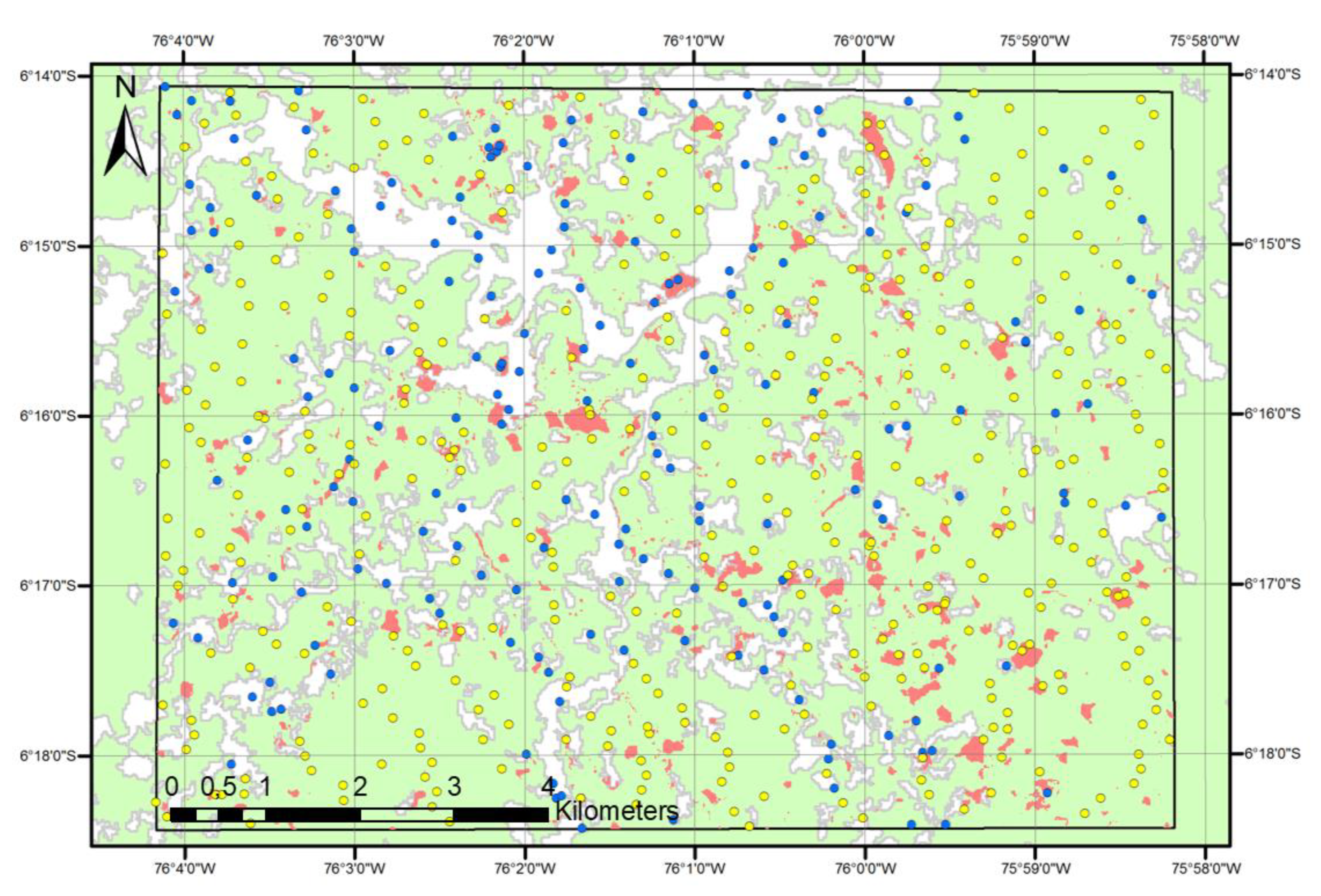
The aim of this study is to analyze if the joint use of SAR (S-1) and optical (S-2 and L8) time series data in forest monitoring approaches can increase forest disturbance detection accuracies in the humid tropics. Forest disturbance maps from SAR and optical data are highly complementary, in that they detect different disturbed forest areas. Therefore, the assumption was that higher accuracy values can be obtained by merging detections from both sensor types. In this study, we demonstrate this at two humid tropical forest test sites located in Peru and in Gabon. Our approach includes the generation of a benchmark forest/non-forest mask, which serves as the starting point for the forest disturbance mapping. Separate forest disturbance maps are then calculated from the SAR and optical time series. The final forest disturbance maps combine the forest disturbance results from SAR and optical time series by a simple union process. The benchmark forest/non-forest masks and all the forest disturbance maps (SAR, optical, combined) are validated with a set of sample plots that were visually interpreted in VHR and HR imagery.

State-of-the-Art

Forest Disturbance Monitoring with Optical Data

The opening of the U.S. Geological Survey (USGS) Landsat data archive in 2008 [9] and the launch of new satellite missions with an open data policy, such as ESA’s Sentinel Missions [10], has formed the basis for time series analysis of optical satellite data at high spatial and high temporal resolution [9,11,12,13]. Although the Sentinel-2 Multi Spectral Instrument (MSI) and the Landsat 8 Operational Land Imager (OLI) bands are not fully compatible in terms of radiometry, recent investigations on radiometric consistency between the two sensors revealed a high correlation between corresponding bands. Dense optical image time series allow for developing new Land Use and Land Cover (LULC) mapping approaches and novel methods for detecting dynamic and gradual, as well as long-term, change processes.

Satellite systems that operate at daily acquisition [14] rates, such as MODIS, can achieve consistent temporal coverage, even in tropical regions. But small disturbances are largely omitted due to the coarse spatial resolution of 250–500 m [15]. Many different algorithms have been proposed to detect forest changes while using time series of medium spatial resolution optical satellite imagery [16,17,18,19,20,21,22,23,24,25]. In the last decade, yearly deforestation mapping and the derivation of deforestation rates have become operational at global [1] and national level e.g., [2,16,17], but there is still only fragmented information available on the extent and magnitude of small forest disturbance and forest degradation [18]. As stated in the GOFC-GOLD REDD sourcebook [19], measuring forest degradation or forest regrowth and related forest carbon stock changes is more challenging than measuring deforestation alone, since degradation monitoring requires more frequent and better imagery and processing.

Cloud cover strongly influences tropical forest disturbance detection accuracies in both space and time [4]. When there are temporal gaps in the time series, rapid vegetation recovery can obscure the signs of disturbance events [20]. Previous studies using multiple years of cloud-free Landsat data in less cloudy regions showed that the regrowth of trees rapidly masks the spectral signature, even of forest clear cuts [21,22]. Thus, a higher percentage of forest disturbances can only be detected with dense time series of optical data. Dense time series are essential for the continued development of near real-time monitoring systems, such as the Global Forest Watch Humid Tropical Forest Alerts [8], and can provide much needed alert information on location and exact timing of illegal logging activities [23].

In terms of methodology, we can divide the time series analysis methods that were used for forest change detection into four broad categories: (1) threshold based change detection; (2) curve fitting; (3) trajectory fitting; and, (4) trajectory segmentation. Existing algorithms often use a combination of these categories. A more detailed description and comparison of these categories can be found in [24]. Thresholding procedures that separate forest from non-forest or intact from degraded forest in a time series are used in the Vegetation Change Tracker (VCT) and Global Forest Watch algorithm [8,25]. Curve fitting approaches for monitoring forest dynamics have been applied in several studies [26,27]. A large number of forest monitoring approaches today are based on trajectory fitting and trajectory segmentation. Most of the disturbance types show a distinct temporal behavior before and after a degradation event, resulting in a “characteristic spectro-temporal signature” that can be exploited to detect and classify forest changes [22]. Trajectory fitting and segmentation algorithms include LandTrendr, Breaks For Additive Season, and Trend (BFAST) and the Continuous Change Detection and Classification (CCDC) algorithm [28,29,30,31]. The dense time series of satellite data also allow to detect forest disturbances from harmonic regression models. The Exponentially Weighted Moving Average Change Detection (EWMACD) algorithm and its evolution, the dynamic algorithm Edyn [32,33], use the residuals from harmonic regression over many years of Landsat data in conjunction with statistical quality control charts to signal vegetation changes. As a conclusion from the literature review, we can state that algorithms that try to detect lesser-magnitude or small-scale disturbances show higher levels of commission error.

Forest Disturbance Monitoring with SAR data

SAR-based forest monitoring approaches are among the most promising remote sensing approaches for the NRT mapping of forest disturbances in the tropics, thanks to the ability of SAR to operate in all weather conditions at any time of day or night. However, SAR data based approaches for forest disturbance mapping have not been well developed yet and operational applications have not yet been implemented [8]. The release of the global JERS, PALSAR, and PALSAR-2 mosaics at 25 m resolution has fostered studies that are related to forest monitoring with SAR. ALOS PALSAR mosaics were used to produce the first SAR-based annual (2007–2010) global maps of forest and non-forest cover, from which some maps of forest losses and gain were generated based on thresholds [34]. Tropical forest change monitoring with SAR data is usually performed by measuring backscatter intensity changes over time. Forest disturbances and regrowth have been assessed atsubcontinental scale over South-East Asia while using SAR intensity changes [35]. Indirect approaches relate the backscatter signal to forest biomass using regional empirical regression models [36,37] and then calculate biomass changes over time. Such an approach has been tested in a small area in Central Mozambique [38]: forest aboveground biomass (AGB) is estimated from SAR backscatter at two periods, and then changes in AGB are determined by subtracting the two estimates. This method is relevant in the context of REDD+ measurement, reporting, and verification (MRV), because both disturbance areas and biomass losses are estimated in one approach. However, the method suffers from error propagation, as errors in both maps may be summed. Applications that are based on ALOS PALSAR data are constrained by the small number of available observations: one observation per year in the case of the mosaics and one observation every 42 days at best with the original data. Most applications are therefore limited to bi-temporal analyses.

Other SAR based forest disturbance mapping approaches use three-dimensional (3D) information from radargrammetry and InSAR to detect gaps in the forest canopy [39,40,41]. The complementarity of SAR sensors of different frequency for forest disturbance monitoring was demonstrated at a test site in the Republic of the Congo for Sentinel-1 C-band and TerraSAR-X data [24].

C-band SAR data is less suited for forest disturbance assessment and above-grove biomass estimation than L-band SAR due to its shorter wavelength, which limits the penetration into the canopy (as evidenced in [42]). C-band SAR has therefore been used to a much lesser degree than L-band data in past forest monitoring studies. However, the dense time series of the Sentinel-1 constellation offer a unique opportunity to systematically monitor forests at a repeat cycle of six to 12 days, depending on the data type and location. In addition, the continuity of Sentinel data is guaranteed up to 2030 with S-1C/D and S-2C/D, and the next generation of Sentinel satellites is already planned beyond 2030, allowing the development of long-term environmental monitoring systems.

A number of recent studies have already used Sentinel-1 data for forest disturbance mapping. Most of the approaches measure changes in SAR backscatter intensity over time, either directly from image to image or by calculating the coefficient of variation of a data stack for a pre-defined time period. Empirical thresholds are then applied to derive the forest disturbances. Such approaches have been tested for forest disturbance mapping in the Republic of the Congo [14,43] and for mapping forest fire-affected areas in Indonesia [44]. A recent research study at a tropical forest site in Bolivia showed that the Sentinel-1 time series data can provide much more timely detections than Landsat and ALOS PALSAR-2 data [45]. 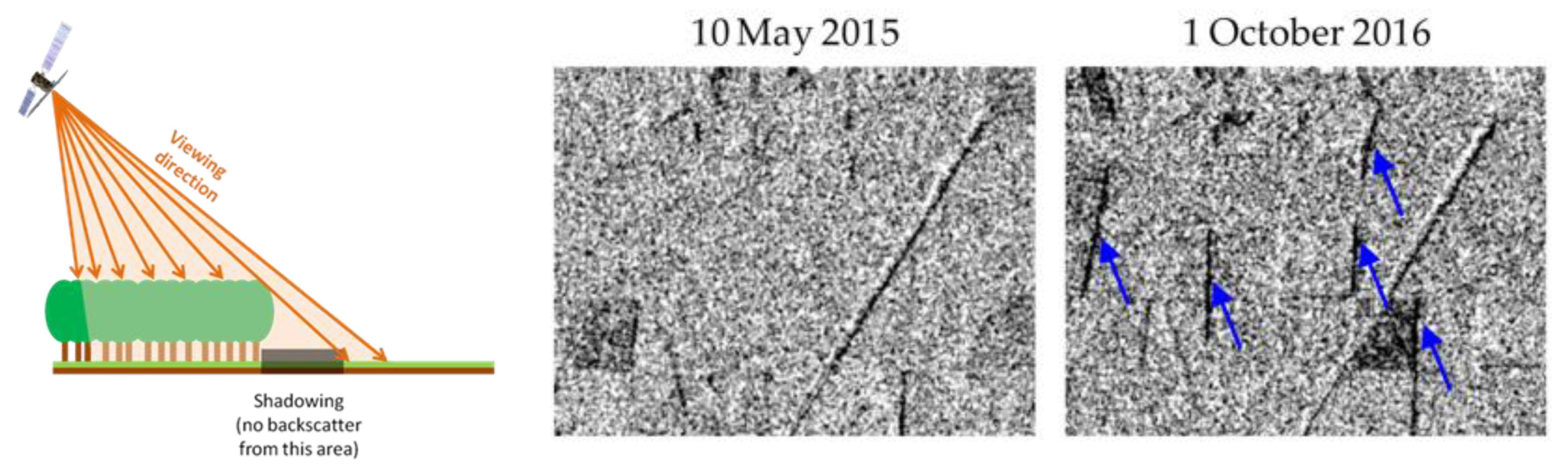Most of the studies for detecting disturbances from Sentinel-1 data assume that forest disturbances are necessarily characterized by a decrease in C-band backscatter within the disturbed area, which does not always seem to be the case [46]. Therefore, a new method that uses the geometric effects of SAR shadowing to detect forest change areas from Sentinel-1 SAR data has been proposed by [47]. Depending on viewing geometry, SAR shadowing occurs at forest edges and new forest edges thus result in new SAR shadows that can be easily detected in the time series. Ascending and descending orbit data are needed to detect new shadows on two sides of the forest disturbance patch. The entire disturbed area is then reconstructed from the newly detected shadows using a convex envelope boundary operator. This new method is used for the SAR based forest disturbance detection in this study and Section 4 describes it in more detail.

Forest Disturbance Monitoring Combining SAR and Optical Data

Optical and SAR data have been combined in remote sensing applications for many years [48,49]. Combination methods on a data-level that preserve spectral as well as spatial characteristics of both sensors are difficult to design. The combination of SAR and optical data on a result-level avoids this problem by classifying each source individually. The results are then combined while using various methods, such as probabilistic theory, evidence theory, fuzzy theory, neural networks, or ensemble learning classifiers. This way, the characteristics of both sensors can successfully be preserved [49,50].

There are a number of recent studies that argue in support of a combined use of SAR and optical data for tropical forest monitoring [3,50,51,52,53]. Recent results indicate that a combined use can improve tropical forest monitoring for burnt area detection [14], for forest/non-forest mapping [52,54,55], for biomass assessment [56,57,58], and for deforestation and degradation monitoring [45,51,59]. A combination of ALOS PALSAR data and Landsat data was also used to enhance the discrimination of mature forest, secondary forest, and non-forest areas [60]. A recently presented workflow for near real-time deforestation detection integrates medium resolution optical data and SAR data in a Bayesian approach [45,50]. By integrating optical Landsat 7/8 data with ALOS PALSAR-2 L-band and Sentinel-1 C-band SAR data, deforestation areas in Bolivia were detected with a mean time lag of 31 days, and detections show a user accuracy of 88% and a producer accuracy of 89. The time lag increased by a considerable six weeks when only using Landsat data and by one week when only using Sentinel-1 data [3]. However, the study only focuses on deforestation areas and does not address small forest disturbances that are difficult to detect from medium resolution data, such as Landsat, but require high resolution data instead.

What is still missing in current research developments is an in-depth analysis of forest disturbance detection capabilities that can be achieved by combining data from the Sentinel-2 and Sentinel-1 missions. These two satellite missions currently have the highest temporal coverage of freely available data and provide imagery at high spatial resolution. One reason why these data sets have not been joined more extensively yet could be that many research studies using time series of data rely on processing services, such as Google Earth Engine (https://earthengine.google.com/), where Sentinel-2 surface reflectance data has only been included recently.

2. Material and Methods

2.1. Test Sites

The study is performed at two test sites in humid tropical forest regions: one test site is located in Peru, near the city of Yurimaguas, and the second test site is located in Gabon, near the city of Fougamou.

The Peruvian test site (see Figure 1) covers approximately 6000 km² around the city of Yurimaguas (76°05′W, 5°45′S), which is located at the river Huallaga near the border between the Loreto and San Martin regions. It is the same test site that was previously used to demonstrate the SAR shadow method for forest disturbance detection [47]. Most of the study area lies within the tropical rainforest zone, which is characterized by a mean temperature of all months higher than 18 °C, an annual precipitation of at least 1500 mm, and at most three dry months during winter. In Yurimaguas, the mean long-term temperature is 26 °C and the mean annual rainfall is 2200 mm [61,62]. Only in June, July, August, and September the mean monthly rainfall is lower than 200 mm [61]. The Peruvian test site is intensively used and characterized by shifting cultivation, plantations, and mining activities. The patterns of forest degradation strongly differ in extent and temporal behavior. Areas with traditional subsistence farming based on shifting cultivation typically show forest disturbances smaller than 0.5 ha, which by FAO definition is forest degradation [63]. The forests in the area are partly primary and mostly secondary forests, i.e., previously disturbed forests. Forest/Non-forest maps that follow the FAO forest definition [63] and forest disturbance maps are derived for the entire test site. Due to limited availability of reference data, the validation was performed at a small subset of 88.33 km², which includes the major forest change drivers and is mainly characterized by areas of shifting cultivation and by forest disturbances that are smaller than 0.5 ha in size.

The Gabonese study area (see Figure 2) is approximately 6480 km² large and it extends over parts of the provinces of Ngouine, Ogooue-Maritime and Moyen-Ogooue. It completely lies within the ecological zone of tropical rainforests. In Fougamou (10°35′E, 1°13′S), the largest city in the study area, the climatic conditions are very similar to Yurimaguas with a mean long-term temperature of 26 °C and a mean annual precipitation of 1995 mm with the dry season between June and September, where precipitation does not exceed 100 mm (https://de.climate-data.org/location/32332/#climate-graph). The presence of cloud cover in Gabon is nearly continuous throughout the year. The main drivers for deforestation at the test site are (i) mining activities in the north; (ii) large palm oil plantations in the south; and (iii) agricultural activities along roads and rivers. The main driver for forest degradation is industrial selective logging [64], which occurs in several concession areas and is characterized by a large number of very small forest disturbances (<0.2 ha) and related logging roads [65].

2.2. Data Sets

For Peru, the set of optical images consists of data from Landsat 8 (WRS: 008-064) and Sentinel-2 (granule: 18MUU) from 03/2015–05/2017. We used optical data from 03/2015 to 03/2016 to generate the initial forest/non-forest mask. Forest disturbance mapping is based on all optical and SAR data from 03/2016 to the end of 12/2016. Optical data from 2017 were only used to confirm the mapped disturbances in the confirmation loop that is described in the respective chapter on data processing. Sentinel-1 data is from both ascending and descending relative orbits (orbit 43—ascending; orbit 49—descending). The time interval between two consecutive acquisitions with the same orbit orientation is 24 days. Images in ascending orbit are acquired three days after images in descending orbit. The polarization mode is single VV until the end of 2016. In short, for Peru, we generate a forest/non-forest mask for status March 2016 and a disturbance map for the period March-December 2016.

For Gabon, we used optical data from Landsat 8 (WRS: 185-061) and Sentinel-2 (granule: 32MPD) from 2013 to 2017 and Sentinel-1 SAR data (VV and VH polarizations) from 2015 to 2017. We calculated the initial benchmark forest/non-forest mask based on Landsat 8 data from the year 2013. Initially, we calculated all changes from 2013–2017 from optical data only. For the aim of this study to combine optical and SAR data, we only evaluate the changes between 15 December 2015 and 8 April 2017 in order to have temporally consistent stacks of data from both optical and SAR sensors. In short, for Gabon, we have a FNF map for status 2013 and a forest disturbance map for December 2015–April 2017.

2.3. Pre-Processing

Optical Data Pre-processing

We downloaded all Sentinel-2 data from the Copernicus Data Hub (https://scihub.copernicus.eu), as Level-1C products. Pre-processing of Sentinel-2 data is performed with the Sentinel-2 Reflectance Data Processing module implemented in the JOANNEUM RESEARCH in-house software IMPACT. First, all of the downloaded Level-1C S-2 images are atmospherically corrected to bottom-of-atmosphere (BoA) values using the integrated Sen2Cor processor version 2.5.5 [66]. The aerosol type is set to “rural”, whichbetter fits both test sites then the alternative options “maritime” or “auto”. The atmosphere type and ozone content are set to “auto”, leading to an automatic determination by the algorithm [66]. Subsequently, we resample the 20 m bands to 10 m spatial resolution and then stack all 10 m and 20 m bands to a 10-band output image. Clouds and cloud shadows must be masked out prior to classification to avoid later misclassifications. The Sen2Cor processor also generates a scene classification map based on threshold operations while using different single spectral bands, band ratios, and indices [66]. We use this scene classification to derive final cloud and cloud shadow masks. Areas classified as clouds with either “medium” or “high” probability and areas classified as cloud shadows are extracted from the scene classification and written to a binary mask. This mask is slightly altered by morphological operations (erode, expand), cloud holes are filled, and the masked areas are then removed from the pre-processed S-2 imagery. We also perform a topographic correction that is based on an implementation of the Minnaert correction in IMPACT software [67] using the Shuttle Radar Topography Mission (SRTM) model at 30 m spatial resolution as digital elevation model.

Landsat 8 data are available as surface reflectance products (Level-2 data) through the USGS EarthExplorer (https://earthexplorer.usgs.gov). An accurate cloud mask is also available for each image. It is computed with the CFMask algorithm, which is the C version of the Function of Mask (FMask) algorithm that was developed by [68]. Itperforms an automated object-based cloud and cloud shadow detection in Landsat images [69,70]. Cloud and cloud shadows are removed from the imagery and the Landsat 8 data is resampled to 10 m cell size to be consistent with S-2 spatial resolution.

When images from different sensors are used in a combined time series, geometric consistency is a requisite, since geometric errors almost certainly lead to misclassifications [12]. To register the L8 scenes to the S-2 scenes, we use a fully automated multi-modal image matching algorithm that is based on the concept of mutual information maximization [71].

SAR Data Pre-processing

We processed S-1 SAR data using the “s1tiling processing chain” [72], based on the free Orfeo Toolbox (website: www.orfeo-toolbox.org). Pre-processing comprised the following steps: calibration, orthorectification, multi-image filtering [73,74,75], and splitting into the S-2 tiling grid that is referenced to the U.S. Military Grid Reference System (MGRS). The SAR data sets are calibrated to gamma nought backscatter and orthorectified to 10 m resolution in UTM projection that was based on the SRTM model at 30 m resolution. A multi-image filter [74,75] is applied to decrease the speckle effect and to enhance the equivalent number of looks (ENL). A 3 × 3 spatial window was chosen, and each image was filtered only with the images acquired before its own acquisition date, in order to simulate NRT conditions. Further details on the pre-processing of the SAR data can be found in chapter 2.2.1 of [47].

2.4. Main Processing

The overall workflow is depicted in Figure 3 and explained in detail in the respective chapters below.

2.4.1. Generating an Initial Benchmark Forest Mask

The first step of the forest disturbance monitoring workflow is the generation of an initial benchmark forest/non-forest (FNF) mask (see Figure 3), which accurately represents the forest area right at the beginning of the change detection window. The forest masks were derived with slightly different approaches for Gabon and Peru, due to differences in optical data availability. For the Peru test site, the FNF map is based on all optical data from 03/2015-03/2016, in total 13 images from both Landsat 8 and Sentinel-2 sensors. We started with deriving training data for the FNF classification from a low cloud covered Sentinel-2 scene from 10 March 2016 and from RapidEye and VHR data sets from 2015 and early 2016 (for details see Section 2.4.3). Subsequently, we used the Sentinel-2 scene from 10 March 2016 and the training data (forest and non-forest areas) to train a classifier and derive a classification model with the Orfeo Toolbox (www.orfeo-toolbox.org). We then tested different classification approaches (Maximum Likelihood, Random Forest, Normalized Difference Vegetation Index (NDVI), and Normalized Difference Infrared Index (NDII7) thresholding) and different input data options, and found the Random Forest based machine learning classifier to deliver the best overall accuracies for the benchmark FNF map [76]. We then applied the Random Forest classification model derived from the 10 March 2016 Sentinel-2 scene to all other pre-processed optical images from 03/2015-03/2016, resulting in 13 individual FNF maps with class categories “forest”, “non-forest”, and “no data” (e.g., clouds). For the final FNF map, we apply a weighted majority approach, where FNF masks that lie near the reference date (10 March 2016) in the temporal domain are attributed the highest weights. This weighting approach increases the overall accuracy of the FNF map by 3% [76].

For Gabon, we calculated the FNF mask for the benchmark year 2013. This reference year was a specification from the related project. In 2013, Sentinel-2 data was not yet available. Therefore, the FNF mask in Gabon is solely based on Landsat 8 data. For the FNF mask classification, we chose the Landsat 8 scene with lowest cloud cover in 2013 (02.08.2013). We collected the required training data (forest and non-forest areas) from VHR image chips that were distributed over the test site and then used the Random Forest classifier of OrfeoToolbox to train and classify the Landsat 8 scene while using all Landsat 8 spectral bands. The remaining cloud holes were filled with the classification results of additional scenes with low cloud cover (01.07.2013; 17.07.2013) to guarantee a complete coverage of the final FNF mask.

2.4.2. Disturbance Detection

Optical data

Both of the study areas are located in the humid tropics, where the seasonality of the spectral signal of forests is much less pronounced than for dry tropical forests or temperate forests. Therefore, the applied change detection method does not need to account for seasonality as in the dry tropics [77], and we can apply straightforward thresholding approaches. Single spectral bands usually show higher variance in time series than indices, which is why indices are commonly used as input data to times series analyses. Our initial tests revealed that NDVI and NDII7 (Normalized Difference Infrared Index with Landsat band 7: (band4-band7) / (band4 + band7)) show the best overall accuracies for forest disturbance detection. However, the Landsat 8 surface reflectance data in Peru and Gabon showed artifacts in the optical bands that, according to the USGS, were caused by the Global Climate Modeling (GCM) grid’s aerosol values not being correctly interpolated to the Landsat grid. We use the NDII7 index as input to disturbance mapping with Landsat 8 instead of NDVI to bypass this radiometric issue, as NDII7 does not include the optical bands. The NDVI (for Sentinel-2) and NDII7 (for Landsat 8) are individually calculated for all pre-processed and radiometrically adjusted images for the time window 10.03.2016 to 31.12.2016 at the Peruvian test site and for the time window 15.12.2015 to 08.04.2017 at the Gabonese test site. An additional eight weeks are also processed for the optical data disturbance confirmation. All of the pixels with NDVI and NDII7 values exceeding the thresholds indicate a forest disturbance and are therefore named “disturbance indicator” (see Figure 3).

The forest disturbance detection workflow is described in [52] and follows recommendations from other operational approaches [8]. It is based on the temporal behavior of index values and a thresholding approach. From reference data plots, we derive a threshold value for the NDVI and the NDII7, which separates the forested and non-forested areas. When an index value falls below the defined threshold, it is considered to be a preliminary potential forest disturbance detection. At this point, it is still unknown if this detection represents a real forest disturbance, or just remnants of an undetected cloud, a radiometric artifact or simply a false classification in the benchmark FNF map. Therefore, single outlier detection is only considered as a “possible disturbance”. We then developed a confirmation tool to analyze these preliminary disturbance detections in time. Subsequent observations are used to either confirm the disturbance detection if their spectral values are also below the defined threshold or to reject the detection if spectral values of subsequent images are above the valid threshold. If three consecutive outliers are detected, the forest disturbance is confirmed and added to the final disturbed forest output file (referred to as “Optical Only” in subsequent text).

The final optical data based forest disturbance file is a 10 m raster product that sums all of the confirmed changes within the forest area for the observation period. A minimum mapping unit of 0.04 ha is applied.

SAR data

The near real time forest disturbances detection method based on SAR data has been described in detail in [47] and was successfully tested in Peru. Classical methods for SAR based forest change detection are based on the hypothesis that the radar backscatter decreases when forest disturbances occur. However, backscatter does not necessarily decrease, because soil moisture and/or trees that remain on the ground can also lead to an increase of the radar backscatter [46].

To overcome this problem, the new method [47] is based on the detection of radar shadowing. Shadowing occurs in radar images because of the particular side-looking viewing geometry of radar systems. A shadow in a radar image is an area that cannot be reached by any radar pulse. The incidence angle and the tree height, shadows created by trees at the border between forest and non-forest areas, can be observed in high-resolution radar images, depending on the viewing direction (Figure 4). A sudden drop in backscatter in the radar time series characterizes new radar shadows. Thanks to the purely geometrical nature of the shadowing effects, this decrease of backscatter is expected to be persistent over time. New shadows should consequently remain visible for a long time and are easily detectable when dense time series of radar data, such as Sentinel-1 time series, are available. Ascending and descending orbit data are needed to detect new shadows on two sides of a forest disturbance patch. The entire disturbed area is then reconstructed from the newly detected shadows while using a convex envelope boundary operator. For every SAR image of the time series, new SAR shadows are identified and combined with previous/subsequent detections in the complementary orbit direction. If a disturbed area can be reconstructed, it is written to a disturbance detection file for this specific date and the area is removed from the forest area in the FNF mask. The single date detections are then summed over the time window of interest to a final SAR disturbance map (“S1 Only”).

Combination of Optical and SAR

SAR and optical data are combined by merging the final forest disturbance maps of both sensor types. For the chosen time window of interest, we processed and confirmed the forest disturbance detections for each sensor type separately (see workflow illustration Figure 3), and we then combined the sensor type specific forest disturbance map results with a simple “Union” process in a Geographic Information System. The union process joins all detections of the two forest disturbance maps, thus increasing the overall detected disturbed forest area.

2.4.3. Evaluation Concept for FNF Mapping

The evaluation of the FNF maps is based on systematic random sampling points [78] that were visually interpreted in VHR image chips (see Figure 5, example of Peru). The VHR image chips were ordered based on a pre-defined systematic sampling grid. Within each grid cell a random sampling was applied. We additionally derived inclusion probabilities and area estimates from the final forest/non-forest classifications since the VHR image chips do not cover the entire mapped area.

Table A1. Confusion matrix for 2016 FNF map of Peru (plots and area weights). Map categories are the rows, reference categories are the columns.

Class	Forest	Non-Forest	Total	Map Area [ha]	Weights
Forest	3663	216	3879	489,899	0.810
Non-Forest	151	980	1131	114,603	0.190
Total	3814	1196	5010
Class	Forest	Non-Forest	Total	User	CI at 95%	Producer	CI at 95%	Overall	CI at 95%
Forest	0.765	0.045	0.810	0.944	±0.0072	0.968	±0.0046	0.930	±0.0070
Non-Forest	0.025	0.164	0.190	0.867	±0.0198	0.785	±0.0222
Total	0.790	0.209	1.000

and

Table A2. Confusion matrix for 2013 FNF map of Gabon (plots and area weights). Map categories are the rows, reference categories are the columns.

Class	Forest	Non-Forest	Total	Map Area [ha]	Weights
Forest	5561	37	5598	648,460	0.947
Non-Forest	43	359	402	36422	0.053
Total	5604	396	6000
Class	Forest	Non-Forest	Total	User	CI at 95%	Producer	CI at 95%	Overall	CI at 95%
Forest	0.941	0.006	0.947	0.947	±0.0021	0.994	±0.0017	0.988	±0.0026
Non-Forest	0.006	0.048	0.054	0.893	±0.0303	0.884	±0.0332
Total	0.946	0.054	1.000

provide the confusion matrices for Peru including all accuracy measures (overall, user, and producer accuracy; confidence levels).

2.4.4. Evaluation Concept for Disturbance Mapping

We use two different approaches to validate the disturbance maps: a plot-based approach based on digitized disturbance patches and an area-based approach based on stratified random sample points. Both validation approaches are meaningful for different assessments. The plot-based approach is viable for example in an alert system, where it is more important to pinpoint the location, where something is happening than delineating the exact outline. The area-based approach is needed e.g., in the frame of REDD reporting, where the disturbed forest area is needed as activity data.

For the plot-based approach, we calculate the detected area percentage for each reference plot. A plot is considered to be correctly detected if a user defined percentage of its area is detected. For Peru and Gabon, we use a 10% threshold. If a percentage of the plot area higher than 10% is detected by the disturbance mask, the plot is considered correctly identified. For Peru, the 148 reference disturbance plots cover an area of roughly 108 ha. In terms of plot size, only 34 of the 142 plots are larger than 1 ha and 35 are smaller than 0.2 ha. For Gabon, the 362 reference disturbance plots cover an area of 6420 ha. In terms of plot size, 51 plots are larger than 1 ha and 166 are smaller than 0.2 ha. These patches are an arbitrary subset based on available VHR data and they do not necessarily represent the whole test site.

The area-based approach allows for the computation of user, producer, and overall accuracy based on the representative areas of reference plots in each stratum (non-forest, undisturbed forest, and disturbed forest). We performed a visual interpretation of HR and VHR (RapidEye, Worldview-2, Spot-6) data in order to obtain reliable ground truth data for this assessment. For Peru, we used RapidEye data from 14 August 2016, ArcGIS Basemap (WorldView-2) data from 20.06.2015, Google Earth imagery from 2015 and 2018, and all Sentinel-2 data from 10.01.2016 to 25.12.2016. The area-based validation was carried out at a sub-region covering 88.33 km² for which RapidEye data was available. For Gabon, we visually interpreted a combination of RapidEye, WorldView and Spot-6 data and the full Sentinel-2 time series for the time window 12/2015–4/2017. The validation was carried out at the full extent. The overall number of plots and the plots per stratum are based on recommendations for land cover accuracy estimation [79,80]. The disturbance result from the “Union” combination was used to estimate the map areas per stratum. For Peru, we sampled a total of 575 reference points within a subset of the map (see Figure 6) with 75 sample points for the stratum “D” (disturbed forest), 114 sample points for stratum “NF” (non-forest) and 384 sample points for stratum “F” (undisturbed forest). The respective area weights are provided in

Table A3. “S1 Only” Peru disturbance map validation.

Class	F	D	NF	Total	Map Area [ha]	Weights
F	330	15	57	402	6693.80	0.758
D	2	38	19	59	331.79	0.038
NF	18	0	96	114	1807.39	0.205
Total	350	53	172	575	8832.98	1.000
Class	F	D	NF	Total	User	Producer	Overall
F	0.622	0.028	0.107	0.758	0.821	0.949	0.819
D	0.001	0.024	0.012	0.038	0.644	0.461
NF	0.032	0.000	0.172	0.205	0.842	0.590
Total	0.656	0.052	0.292	1.000

. For Gabon, we sampled a total of 855 reference points within 14 subset areas of the map, for which also VHR imagery was available. The 855 total plots are composed of 112 sample points for stratum “D_large” (disturbed forest areas ≥ 25 ha), 81 sample points stratum “D_small” (disturbed forest areas < 25 ha), 121 sample points for stratum “NF” (non-forest) and 541 sample points for stratum “F” (undisturbed forest).

Table A9. “S1 Only” disturbance map validation Gabon.

Class	F	Dlarge	Dsmall	NF	Total	Map Area [ha]	Weights
F	530	51	20	41	642	46,394.94	0.884
Dlarge	0	55	0	1	56	1732.60	0.033
Dsmall	7	0	28	1	36	1179.65	0.023
NF	7	0	0	114	121	3169.56	0.060
Total	544	106	48	157	855	52,476.75	1.000
Class	F	Dlarge	Dsmall	NF	Total	User	Producer	Overall
F	0.730	0.070	0.028	0.056	0.884	0.826	0.989	0.837
Dlarge	0.000	0.032	0.000	0.001	0.033	0.982	0.316
Dsmall	0.004	0.000	0.017	0.001	0.022	0.778	0.388
NF	0.003	0.000	0.000	0.057	0.060	0.942	0.497
Total	0.738	0.103	0.045	0.115	1.000

provides the respective area weights.

For the area-based accuracy assessment, we calculate the confusion matrices for the three, respectively, four, different strata and for all sensor specific disturbance maps—i.e., “S1 only”, “Optical only”, and “Union”. The confusion matrices are provided in Table A3,

Table A4. “Optical Only” Peru disturbance map validation.

Class	F	D	NF	Total	Map Area [ha]	Weights
F	331	27	70	428	6693.80	0.758
D	1	26	6	33	331.79	0.038
NF	18	0	96	114	1807.39	0.205
Total	350	53	172	575	8832.98	1.000
Class	F	D	NF	Total	User	Producer	Overall
F	0.586	0.048	0.124	0.758	0.773	0.946	0.788
D	0.001	0.030	0.007	0.038	0.788	0.382
NF	0.032	0.000	0.172	0.205	0.842	0.569
Total	0.620	0.077	0.303	1.000

and

Table A5. “Union” Peru disturbance map validation.

Class	F	D	NF	Total	Map Area [ha]	Weights
F	329	5	52	386	6693.80	0.758
D	3	48	24	75	331.79	0.038
NF	18	0	96	114	1807.39	0.205
Total	350	53	172	575	8832.98	1.000
Class	F	D	NF	Total	User	Producer	Overall
F	0.646	0.010	0.102	0.758	0.852	0.950	0.842
D	0.002	0.024	0.012	0.038	0.640	0.710
NF	0.032	0.000	0.172	0.205	0.842	0.602
Total	0.680	0.034	0.286	1.000

for Peru and Table A9,

Table A10. “Optical Only” disturbance map validation Gabon.

Class	F	Dlarge	Dsmall	NF	Total	Map Area [ha]	Weights
F	516	7	29	21	573	46,394.94	0.884
Dlarge	4	99	0	4	107	1732.60	0.033
Dsmall	17	0	19	18	54	1179.65	0.023
NF	7	0	0	114	121	3169.56	0.060
Total	544	106	48	157	855	52,476.75	1.000
Class	F	Dlarge	Dsmall	NF	Total	User	Producer	Overall
F	0.796	0.011	0.045	0.032	0.884	0.901	0.985	0.892
Dlarge	0.001	0.031	0.000	0.001	0.033	0.925	0.739
Dsmall	0.007	0.000	0.008	0.007	0.022	0.352	0.150
NF	0.003	0.000	0.000	0.057	0.060	0.942	0.580
Total	0.808	0.041	0.053	0.098	1.000

and

Table A11. “Union” disturbance map validation Gabon.

Class	F	Dlarge	Dsmall	NF	Total	Map Area [ha]	Weights
F	509	2	10	20	541	46,394.94	0.884
Dlarge	4	104	0	4	112	1732.60	0.033
Dsmall	24	0	38	19	81	1179.65	0.023
NF	7	0	0	114	121	3169.56	0.060
Total	544	106	48	157	855	52,476.75	1.000
Class	F	Dlarge	Dsmall	NF	Total	User	Producer	Overall
F	0.832	0.003	0.016	0.033	0.884	0.941	0.987	0.930
Dlarge	0.001	0.031	0.000	0.001	0.033	0.929	0.904
Dsmall	0.007	0.000	0.011	0.005	0.022	0.469	0.392
NF	0.003	0.000	0.000	0.057	0.083	0.942	0.593
Total	0.843	0.034	0.027	0.096	1.000

for Gabon. We estimate the products’ user and producer accuracies from the error matrix using the estimated area proportions and Equations (6)–(8) from [79]. The benchmark non-forest mask is an essential a priori information, and errors in forest/non-forest masking strongly influence forest disturbance detection accuracies. We therefore derived a second set of confusion matrices, where all non-forest areas and misclassified sample points related to FNF mask errors are removed from the reference data set and where area weights of the strata are then recalculated accordingly, in order to evaluate the methods’ accuracies independently from forest mask errors. The results are provided in

Table A6. “S1 Only” Peru disturbance method validation (only forest area).

Class	F	D	Total	Map Area [ha]	Weights
F	330	15	345	5805.32	0.963
D	2	38	40	225.61	0.037
Total	332	53	385	6030.93	1.000
Class	F	D	Total	User	Producer	Overall
F	0.921	0.042	0.963	0.957	0.998	0.956
D	0.002	0.036	0.037	0.950	0.459
Total	0.923	0.077	1.000

,

Table A7. “Optical Only” Peru disturbance method validation (only forest area).

Class	F	D	Total	Map Area [ha]	Weights
F	331	27	358	5805.32	0.963
D	1	26	27	225.61	0.037
Total	332	53	385	6030.93	1.000
Class	F	D	Total	User	Producer	Overall
F	0.890	0.073	0.963	0.925	0.998	0.926
D	0.001	0.036	0.037	0.963	0.332
Total	0.891	0.109	1.000

and

Table A8. “Union” Peru disturbance method validation (only forest area).

Class	F	D	Total	Map Area [ha]	Weights
F	329	5	334	5805.32	0.963
D	3	48	51	225.61	0.037
Total	332	53	385	6030.93	1.000
Class	F	D	Total	User	Producer	Overall
F	0.948	0.014	0.963	0.985	0.998	0.983
D	0.002	0.035	0.037	0.941	0.710
Total	0.950	0.050	1.000

for Peru and

Table A12. “S1 Only” disturbance method validation Gabon (only forest area).

Class	F	Dlarge	Dsmall	Total	Map Area [ha]	Weights
F	530	51	20	601	42,399.24	0.896
Dlarge	0	55	0	55	2169.83	0.046
Dsmall	7	0	28	35	2763.15	0.058
Total	537	106	48	691	47,332.23	1.000
Class	F	Dlarge	Dsmall	Total	User	Producer	Overall
F	0.790	0.076	0.030	0.896	0.882	0.985	0.883
Dlarge	0.000	0.046	0.000	0.046	1.000	0.376
Dsmall	0.012	0.000	0.047	0.058	0.800	0.610
Total	0.802	0.122	0.077	1.000

,

Table A13. “Optical Only” disturbance method validation Gabon (only forest area).

Class	F	Dlarge	Dsmall	Total	Map Area [ha]	Weights
F	516	7	29	552	42,399.24	0.896
Dlarge	4	99	0	103	2169.83	0.046
Dsmall	17	0	19	36	2763.15	0.058
Total	537	106	48	691	47,332.23	1.000
Class	F	Dlarge	Dsmall	Total	User	Producer	Overall
F	0.837	0.011	0.047	0.896	0.935	0.966	0.912
Dlarge	0.002	0.044	0.000	0.046	0.961	0.795
Dsmall	0.028	0.000	0.031	0.058	0.528	0.396
Total	0.867	0.055	0.078	1.000

and

Table A14. “Union” disturbance method validation Gabon (only forest area).

Class	F	Dlarge	Dsmall	Total	Map Area [ha]	Weights
F	509	2	10	521	42,399.24	0.896
Dlarge	4	104	0	108	2169.83	0.046
Dsmall	24	0	38	62	2763.15	0.058
Total	537	106	48	691	47,332.23	1.000
Class	F	Dlarge	Dsmall	Total	User	Producer	Overall
F	0.875	0.003	0.017	0.896	0.977	0.973	0.955
Dlarge	0.002	0.044	0.000	0.046	0.963	0.928
Dsmall	0.023	0.000	0.036	0.058	0.613	0.675
Total	0.899	0.048	0.053	1.000

for Gabon).

3. Results

3.1. Results of Benchmark Forest/Non-Forest Masking

According to the FNF maps, at the Peru site 81.0% of the area is forest and 19.0% is non-forest, at the Gabon site 94.7% is forest and 5.3% is non-forest. These values were used for the sampling design and to calculate the respective plot weights. In total, we interpreted 5010 samples for Peru and 6000 samples for Gabon.

Table 1. Forest/Non-Forest mask validation Peru and Gabon.

	User Accuracy		Producer Accuracy		Overall Accuracy
class	Peru	Gabon	Peru	Gabon	Peru	Gabon
F	0.944	0.947	0.968	0.994	0.930	0.988
NF	0.867	0.893	0.785	0.884

summarizes the main validation results. The user and producer accuracies for forest are very high, while the values for NF are considerably lower. However, the overall accuracies are also high due to the large share of forest (0.93 for Peru and 0.99 for Gabon). Table A1 and Table A2 provide the individual confusion matrices including all accuracy measures.

3.2. Results of Forest Disturbance Mapping in Peru

The three different disturbance results from the “S1 Only” approach, the “Optical Only” approach, and the “Union” approach show very different results in terms of overall detected disturbed forest area. This is shown in Figure 7 and

Table 2. Area of detected forest disturbances at the Peru validation site for each mapping approach.

Mapping Approach	Detected Area of Forest Disturbances in ha
S1 Only	248.77
Optical Only	153.90
S1/Optical Union	331.79
S1/Optical Intersect Area	70.88
Adjusted Area Estimate (Reference)	225.61

. The “Union” approach detects almost twice the area of the “Optical Only” approach. The overlapping area of the “S1 Only” and “Optical Only” disturbance maps (yellow areas in Figure 7) is only 70.88 ha, which explains why the “Union” disturbance area is significantly larger than in the two single sensor based disturbance maps.

We use two different approaches to estimate the final disturbance map accuracies. The first accuracy assessment approach is targeted to analyze detection accuracy by disturbance patch size. Disturbance patch size is a critical issue in forest disturbance mapping but it is seldom addressed in publications on forest monitoring. Many studies only map disturbances larger than 0.5 ha and thus only focus on deforestation and do not include small and patchy forest degradation. In our analysis, a disturbance patch is considered detected when > 10% of the disturbed patch area is mapped. The results for Peru are shown in

Table 3. Detection accuracy per disturbance patch size for Peru.

Plot Size	Number of Disturbance Areas	S1 Only	Optical Only	Union
>1 ha	34	0.882	0.853	0.971
0.5–1 ha	36	0.806	0.778	0.889
0.2–0.5 ha	43	0.698	0.674	0.884
<0.2 ha	35	0.486	0.657	0.800
all sizes	148	0.716	0.736	0.885

; those for Gabon are shown in

Table 4. Detection accuracy per disturbance patch size for Gabon.

Plot Size	Number of Disturbance Areas	S1 Only	Optical Only	Union
>1 ha	51	0.686	0.647	0.784
0.5–1 ha	44	0.523	0.364	0.636
0.2–0.5 ha	101	0.248	0.277	0.416
<0.2 ha	166	0.157	0.175	0.295
all sizes	362	0.301	0.293	0.530

.

The second accuracy assessment is based on the stratified random sampling approach described in detail in Section 2.4.4.

Table 5. Disturbance map validation for Peru.

Peru disturbance map validation including NF class:
	User Accuracy			Producer Accuracy			Overall Accuracy
class	S1 Only	Optical Only	Union	S1 Only	Optical Only	Union	S1 Only	Optical Only	Union
F	0.821	0.773	0.852	0.949	0.946	0.950	0.819	0.788	0.842
D	0.644	0.788	0.640	0.461	0.382	0.710
NF	0.842	0.842	0.842	0.590	0.569	0.602
Peru disturbance map validation only within the forest area (method validation):
	User Accuracy			Producer Accuracy			Overall Accuracy
class	S1 Only	Optical Only	Union	S1 Only	Optical Only	Union	S1 Only	Optical Only	Union
F	0.957	0.925	0.985	0.998	0.998	0.998	0.956	0.926	0.983
D	0.950	0.963	0.941	0.459	0.332	0.710

and

Table 6. Disturbance map validation for Gabon.

Gabon disturbance map validation including NF class:
	User Accuracy			Producer Accuracy			Overall Accuracy
class	S1 Only	Optical Only	Union	S1 Only	Optical Only	Union	S1 Only	Optical Only	Union
F	0.826	0.901	0.941	0.989	0.985	0.987	0.837	0.892	0.930
Dlarge	0.982	0.925	0.929	0.316	0.739	0.904
Dsmall	0.778	0.352	0.469	0.388	0.150	0.392
NF	0.942	0.942	0.942	0.497	0.580	0.593
Gabon disturbance map validation only within the forest area (method validation):
	User Accuracy			Producer Accuracy			Overall Accuracy
class	S1 Only	Optical Only	Union	S1 Only	Optical Only	Union	S1 Only	Optical Only	Union
F	0.882	0.935	0.977	0.985	0.966	0.973	0.883	0.912	0.955
Dlarge	1.000	0.961	0.963	0.376	0.795	0.928
Dsmall	0.800	0.528	0.613	0.610	0.396	0.675

provide summaries of the accuracy estimates. They include two analyses per test site. The first analysis also includes the non-forest areas, thus it reflects the accuracy of the map. The second analysis is only carried out for plots that are forest at the beginning of the disturbance detection window. Non-forest areas and all misclassifications of the FNF map are removed. This reflects the accuracy of the change detection method. Broadly speaking, the first analysis is a map validation, while the second analysis is a method validation. The validations are based on 575 points (including NF) and 385 points (only forest) for Peru, and 855 points (including NF) and 691 points (only forest) for Gabon. For Peru, we differentiated three classes, where F = undisturbed forest; D = disturbed forest; NF = non-forest at the beginning of the disturbance detection window. For Gabon, the disturbed class was split in two classes that were based on the area of disturbance plots: D_large = disturbed forest area ≥ 25 ha; D_small = disturbed forest area < 25 ha. Large area disturbances are mostly related to new palm oil plantations. At the Peru subset, there are no disturbances larger than 25 ha, therefore no subdivision was made. The mapped area of the strata and their respective weights are derived from the “Union” disturbance map. The detailed confusion matrices, including plot numbers and applied area weights, can be found in the Table A3, Table A4, Table A5, Table A6, Table A7 and Table A8 for Peru and Table A9, Table A10 and Table A11 for Gabon. We can calculate adjusted area estimates for each class based on the omission and commission errors and the respective area weights [79].

The above accuracy assessments clearly show that misclassifications in the forest/non-forest map contribute a major component to the overall error of the disturbance maps. When the FNF mask errors are removed, the overall accuracies increase significantly.

4. Discussion

Forest/Non-Forest Mask:

The benchmark FNF maps show good overall accuracies for both the Peru (93.0%) and the Gabon test site (98.8%), but the omission and commission errors for the non-forest class are larger than 10% at both test sites. The overall accuracies for Gabon are similar to those reported by other studies: 98.1% for the national forest map of year 2000 and 95.9% for the Global Forest Watch dataset of year 2000 evaluated at a 1 ha minimum mapping unit and > 30% tree cover [81]. The accuracies are generally lower at the Peru site, with an omission error of 21.5% for the non-forest class. The lower accuracies in Peru seem to be related to a lower total percentage of forest area and a higher complexity of land use at the test site. Non-forest areas at the Peru test site make up 20% of the total area, which is a much higher percentage than at the Gabon test site with 5.6%. Large parts of the forested area are composed of secondary forests with rapid regrowth rates and the overall percentage of forest changes is higher than in Gabon. The primary cause of forest loss in the Loret and San Martin region of Peru where the test site is located is clearing for agriculture and pastures and large-scale industrial oil-palm plantations [2]. A rapid regrowth with shrubs, bushes, and low height trees is very common soon after agricultural clearing. Even from visual interpretation of VHR imagery it is often difficult to decide if an area is already forest regrowth or still non-forest. Non-forest areas are mostly characterized by different forms of agricultural use, but also by shrublands and grasslands.

The situation is different in Gabon, where 88.5% of the entire country is covered by forests and large parts of the forest are still primary forests [81]. Large parts of the test site in Gabon are characterized by homogeneous forests. Non-forest areas are not distributed evenly at the Gabon test site, but they are concentrated around villages and oil palm plantations in the South. These site characteristics largely explain the higher FNF map accuracies at the Gabon site.

The different methodologies that are used to derive the FNF maps could also explain some of the observed errors. The Peru FNF map is based on 13 images spanning 12 months. Some changes that occurred towards the end of the time window might not have been accounted for with the applied majority approach, even if a temporal weighting is applied.

Forest Disturbance Detection:

When interpreting the forest disturbance results, it has to be considered that forest disturbances are quite different in character at both of the test sites. Forest disturbances at the Peru test site are characterized by the logging of mostly secondary forests for subsequent agricultural use, which is in-line with other findings [2]. There is almost no selective logging of individual trees, but the size of forest disturbance areas is mostly small (60% are smaller than 0.5 ha). At the Gabon site, we find three different disturbance types: large-area deforestation for oil palm plantations in the South, small scale logging for subsequent agricultural/urban use near villages, and a large amount of industrial selective logging and logging roads in the forest concession areas. Gabon contributes 4.7 ± 0.9% of total forest loss in the Congo basin [64]. Selective logging is by far the most prominent forest disturbance type in Gabon, which is different to the other Congo Basin countries, where small scale clearing for agriculture is the most important driver of forest loss [64]. In the final disturbance map of the combined approach, 85% of the detected forest disturbance areas are smaller than 0.2 ha and 94% are smaller than 0.5 ha. Disturbance patch size is a critical issue in forest disturbance mapping, but it is seldom addressed in publications on forest monitoring. Many studies only map disturbances that are larger than 0.09 ha [8] to 1 ha [81] and, thus, only focus on deforestation and do not include small and patchy forest degradation. In terms of area changes, a large deforestation for oil-palm plantations contributes approximately 55% of the total forest change area.

When comparing the accuracies based on the stratified sampling of the three approaches in Peru-“S1 Only”, “Optical Only”, and “Union”-we find highest overall accuracies for the “Union” approach (0.84), but differences in overall accuracy are small (“S1 Only”: 0.82, “Optical Only”: 0.79). When comparing SAR and optical results for the forest disturbance class, the “Optical Only” approach shows higher user accuracy and lower producer accuracy than the “S1 Only” approach. However, the producer accuracy is lower than 0.5 for both approaches showing high omission errors for both data types. For the “Union” approach, the producer accuracy increases up to 0.71 suggesting that SAR and optical map results are highly complementary. This is also confirmed by the area statistics. Of the 331.79 ha of disturbance area in the “Union” disturbance map, only 42.70 ha are detected by both “S1 Only” and the “Optical Only” approach. This is only about one-fifth of the recalculated adjusted disturbed forest area (225.61 ha). The remaining area is only detected by one of the two approaches. The area statistics also show that the NDVI and NDII7 thresholds used for the optical approach in Peru are slightly too conservative. Only 153.90 ha are detected as disturbed, which is 30% less than the calculated adjusted area.

The producer accuracy of the NF class in Peru is quite low (0.6), suggesting that parts of the forest area in the benchmark FNF mask are indeed not tree-covered at the beginning of the change detection window. The accuracies at this subset are lower than the overall accuracy of the FNF mask for the entire Peru test site. This can be explained by the higher complexity of land use at the subset. It is also partly a problem of the different minimum mapping units used for generating and validating the FNF mask and the disturbance detection. Misclassifications in the benchmark FNF map can make up a large part of the overall error in disturbance detection. This error can be more important than the errors related to the change detection methodology, since the overall area percentage of forest disturbances in one year is only very small. This highlights the importance of using accurate and up-to-date benchmark forest masks in operational forest disturbance monitoring.

When we remove the NF class in the second validation approach, the overall and the user accuracies improve considerably. For the “S1 Only” approach, the user accuracy of the disturbed forest increases from 0.64 to 0.95, as many of detected changes turned out to have been non-forest already at the start of the change detection period. These areas are vegetated and often used for agriculture. In the optical images their spectral signals are quite similar to those of forest and are thus misclassified as forest and no change is detected. However, the S1 approach detects a SAR shadow that is related to an existing forest border. In Peru, the S1 disturbance detection starts with the same date as the optical approach. A shadow is detected in the first S1 image of the time series and, thus, a change is written to the change map, even though the shadow was already present before.

In Gabon, of the 15,723 ha detected as disturbed forest in the “Union” approach, only 5241 ha are detected by both of the approaches. However, in Gabon the “Optical Only” approach detects a much larger disturbed area than the “S1 Only” approach—13,763 ha vs. 7201 ha. This effect is mostly caused by the large deforestation area for a palm oil plantation. The applied S1 disturbance detection approach is not suitable for such large disturbance areas, as the detected shadows on both sides are too far apart to reconstruct the disturbance area with a convex envelope boundary operator. Also very small or very narrow patches are difficult to detect with the S1 approach used in this study. If the gap is too small, the distinct shadow is lost and detection fails. Also thin and elongated disturbance patches stretching in the east–west direction are difficult to detect, as the sensor is side-looking from east or west due to its near-polar orbit.

It can also be expected, that due to their smaller pixel size, the S-2 results are better than the results only based on Landsat data. Shortcomings in all optical approaches are problems with regrowth and the selection of appropriate thresholds. Regrowth and cloud cover are the main limitations of optical disturbance monitoring in the tropics, as discussed in the Introduction. A recent study on forest loss monitoring from 2000–2014 in the Congo Basin with Landsat data showed that in Gabon on average only 1.1 cloud-free observations were available per year [64]. Regrowth cannot properly be detected with such a sparse time series.

Several forest change detection maps and accuracy analyses for both Peru and Gabon have been produced by other research teams in recent years. Most of them are based on Landsat data and validations are mostly carried out at Landsat pixel level, i.e., 30 × 30 m [8,64]. In Peru, a Landsat-based national analysis of forest cover loss from 2000 to 2010 revealed that the majority of gross forest cover loss (92.2%) was attributed to clearing for agriculture and tree plantations. The rest was due to natural disturbance, mostly represented by flooding and river meandering (6.0%), and fires (1.5%). The classification was based on training data derived primarily from Landsat composites and forest cover loss was mapped at 30 m Landsat pixel scale. Validation was performed while using a point-based sampling design at Landsat pixel level (30 × 30 m) [2]. The pixels are visually analyzed for forest cover loss while using Landsat (2000) and RapidEye (2011) data at 5 m spatial resolution. The reported producer accuracy for forest loss is 75.4%. This is significantly higher than our “Optical Only” producer accuracy at the Peru test site of 38.2% and similar to the combined map producer accuracy of 71.0%. We assume that the observed differences are primarily related to sampling unit size-30 × 30 m for the analysis vs. 10 × 10 m in our study-and the complexity of land use at our test site subset. The reference plot area we use for the validation is only 11.11% of that used in [2] and our reference data set includes very small disturbances (0.01 ha) that are neglected in the other study.

Peru was also one of the first countries used to demonstrate and validate the near real-time GFW HTFA (Global Forest Watch—Humid Tropical Forest Alerts) methodology [8]. Detected forest loss was grouped by patch size: Loss detection consisting of a single Landsat pixel (approximately 0.1 ha) totaled only 4% of total detected loss, 33% of detected loss patches were less than one hectare, and 63% were larger or equal one hectare in size. The reported user accuracies on a Landsat-pixel level of 30 × 30 m are between 86.5%, when including boundary pixels, and 96.2% with boundary pixels removed [8]. Producer accuracies are not provided in [8], but most of the omitted samples were from tree cover loss patches < 10 ha (= less than 100 Landsat pixels). For a better comparison between our results and the GFW dataset we also derived mapping accuracies for the GFW dataset for the exact same validation plots and time frame at the Peru test site. The dataset is based on the GFW version 1.6 (https://earthenginepartners.appspot.com/science-2013-global-forest/download_v1.6.html) and includes all changes of 2016 (“lossyear” = 2016) clipped with our FNF mask of March 2016. Thus, the time frame for disturbance detections is identical to the observation period we used in this study. Therefore, the results can be directly compared. For geometric congruency, we also performed a geometric adjustment to the S-2 geometry with the same parameters as used for the adjustment of the original Landsat 8 data.

Table 7. Global Forest Watch changes of 2016 (version 1.6).

Class	F	D	Total	Map Area [ha]	Weights
F	331	22	353	5805.32	0.963
D	1	31	32	225.61	0.037
Total	333	53	385	6030.93	1.000
Class	F	D	Total	User	Producer	Overall
F	0.903	0.060	0.963	0.938	0.999	0.939
D	0.001	0.036	0.037	0.969	0.377
Total	0.904	0.096	1.000

shows the GFW validation results. The user accuracies of disturbances are quite comparable between our approaches (“S1 Only”: 0.95, “Optical Only”: 0.963, “Union”: 0.941 from Table 5) and GFW (0.969 from Table 7), especially the “Optical Only” result is very similar, which makes sense, as GFW is also a result based on optical data. The same is true for the overall accuracy values. Producer accuracy of disturbances for the “Optical Only” result is a bit lower than for the GFW result, which is probably due to the very conservative thresholds selected in the assessments. When comparing the GFW result to the “Union” approach however, the producer accuracy of “Union” is much higher (0.71—Table 5) than that of the GFW data set (0.377—Table 7). This clearly shows the added value of including the additional S-1 data. 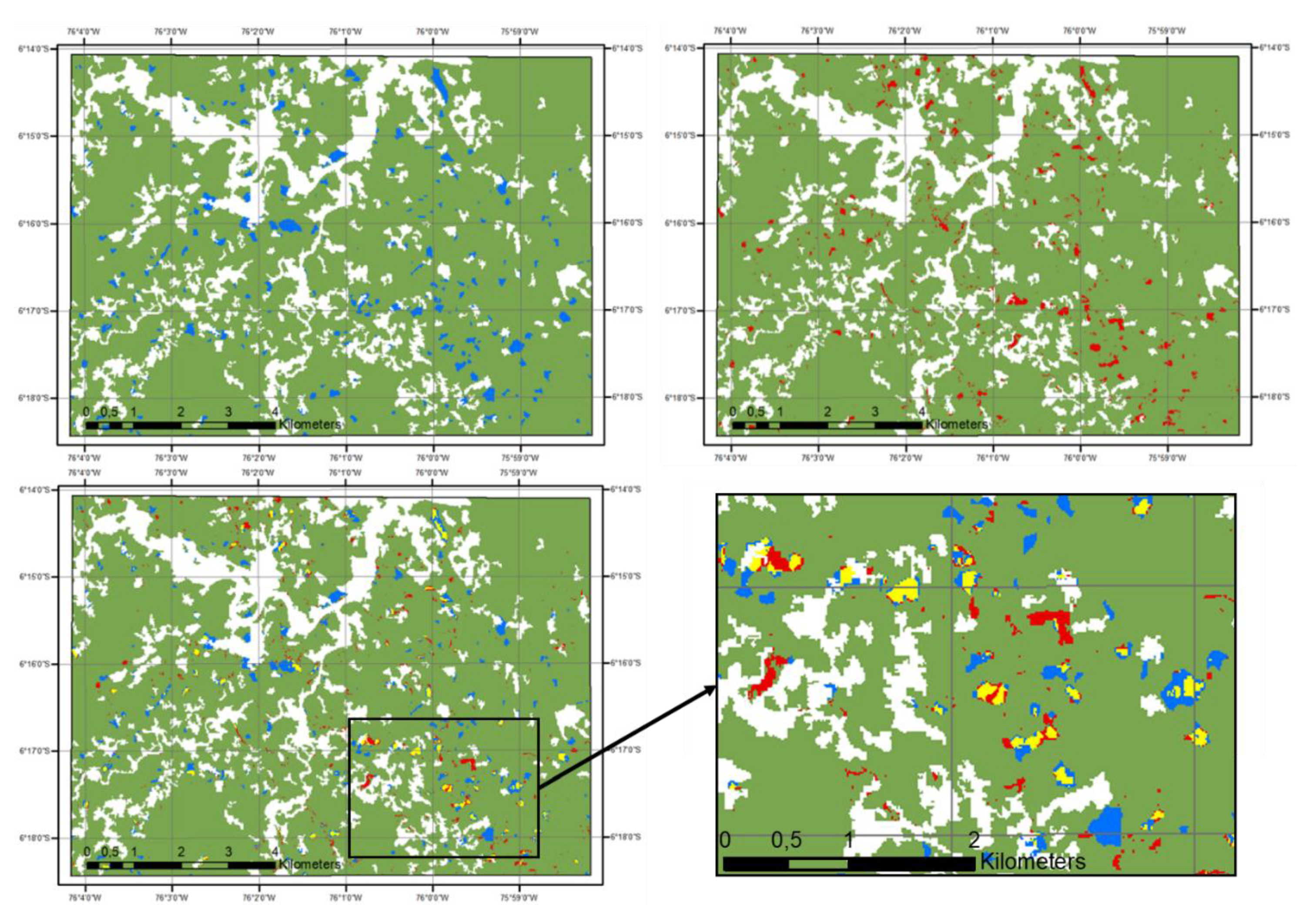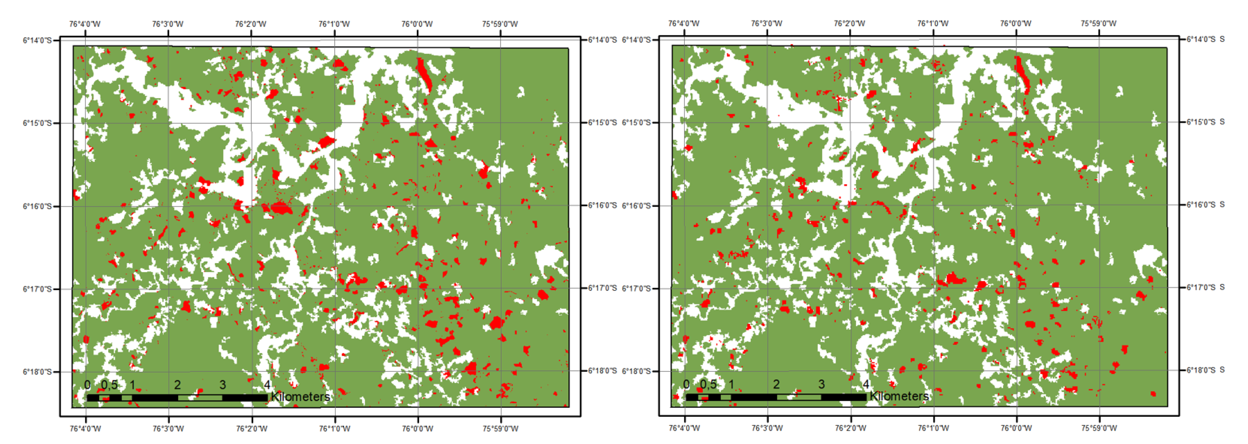Figure 8 provides a visual comparison of the “Union” mapping result and the GFW mapping result.

For Gabon, a recent study compares the forest change estimates from 2000 to 2010 between national forest maps and the Global Forest Change (GFC) map from the University of Maryland [81]. The results indicate that net deforestation is not significantly different to 0, which suggests that the loss of forest is counter balanced by regeneration. The MMU of 1 ha used by GFC in the change analysis [81] strongly differs to that of our presented study, where we detect and validate forest disturbances at a MMU of 0.04 ha. At this spatial level, we also detect small forest disturbances that are typical of industrial selective logging. Selective logging is the most prominent forest disturbance type in Gabon, accounting for more than 60% of forest disturbances [64]. At a 1 ha MMU such small forest disturbance features cannot be detected and, therefore, also not included in the analysis.

Despite or even because of the aforementioned shortcomings, S-1 and optical data are highly complementary. Combining the two data sets significantly increases the accuracy, especially the producer accuracy of disturbances and, as other studies have demonstrated, it also allows for a more rapid detection needed for near real-time alerting [3].

The results show that some forest disturbance patches are indeed detected by both sensor types and related mapping approaches. However, different types of disturbances are often only captured by only one sensor, which confirms the benefit of sensor combination. The contributions of optical and SAR data to the forest disturbance mapping success are variable and they depend on the land use and forest characteristics of a specific site. The dependencies are primarily based on type and typical height of forest (primary, secondary); weather and atmospheric conditions; topography; dominant LU types outside of the forest; change drivers (selective logging, plantations, agriculture, shifting cultivation, fire) and related size of disturbance plots; data availability (ascending, descending for SAR); density of the time series; and regrowth speed, and orientation of the satellite (especially S1) with respect to the disturbance site.

5. Conclusions

Our study confirms, that combining optical and SAR data considerably improves the accuracies of forest disturbance maps. The overall accuracies increase by about 3% at both test sites in Peru and Gabon. Producer accuracies of the disturbance class increase by 13% in Gabon and by 25% in Peru when compared to using only one sensor type. The assessment by disturbance patch size shows, that about 30% of very small disturbances (< 0.2 ha) in Gabon can be detected by using both data sets compared to 17.5/15.7% when using a single sensor. The detection of forest disturbances of this small size from satellite imagery has not been studied yet, as most studies base their validations on Landsat pixel-size validation plots. A combination of S-1 and optical data at data level instead of at result level could proof to be difficult. The detected forest disturbance patches are often not identical but instead highly complementary. This is something to be tested in future research. We could also show that a combination of optical and SAR data at result level does not yield the same amount of accuracy gain at the two test sites (PA increase of 13% in Gabon and of 25% in Peru). More studies are needed in different parts of the tropics and under different forest conditions to better understand the potential and limitations of sensor type combinations for tropical forest disturbance detections.

Further improvements should focus on developing more advanced methods for deriving forest disturbances from SAR and optical data. Simple thresholding, as applied in this study for the optical data, could be replaced by more advanced time series analysis approaches. However, the applicability of such approaches in tropical areas is limited by frequent cloud cover and the lack of dense time series. Here, Planet imagery could play a major role in the future. Commercial Planet data will be available at a daily repetition rate and the new generation of Planet imagery will be spectrally congruent with Sentinel-2. A combination of these two data sets to generate a dense optical time series could stimulate the development of more sophisticated time series analysis tools for tropical forest disturbance monitoring. Such tools are already being used in other fields of remote sensing with good results. In the SAR domain, advancements to the proposed method should focus on an improved detection of larger deforestation patches.. Alternatively, a combination of SAR backscatter-based approaches, which are able to detect large deforestation, and the shadow detection method used in this study could also improve the detection accuracy. Our study supports the use of high resolution, dense time series data for improved forest monitoring, specifically for the detection of small areas of forest disturbance. We could clearly show the high complementarity of the SAR and optical data sets for forest disturbance detection and, therefore, pledge for further development of multi-sensor approaches.

References

1. Hansen, M.C.; Potapov, P.V.; Moore, R.; Hancher, M.; Turubanova, S.A.; Tyukavina, A.; Thau, D.; Stehman, S.V.; Goetz, S.J.; Loveland, T.R.; et al. High-Resolution Global Maps of 21st-Century Forest Cover Change. Science 2013, 342, 850–853. [Google Scholar] [CrossRef] [Green Version]
2. Potapov, P.; Dempewolf, J.; Talero, Y.; Hansen, M.; Stehman, S.; Vargas, C.; Rojas, E.; Castillo, D.; Mendoza, E.; Calderón, A.; et al. National satellite-based humid tropical forest change assessment in Peru in support of REDD+ implementation. Environ. Res. Lett. 2014, 9. [Google Scholar] [CrossRef]
3. Reiche, J.; Hamunyela, E.; Verbesselt, J.; Hoekman, D.; Herold, M. Improving near-real time deforestation monitoring in tropical dry forests by combining dense Sentinel-1 time series with Landsat and ALOS-2 PALSAR-2. Remote Sens. Environ. 2018, 204, 147–161. [Google Scholar] [CrossRef]
4. Hansen, M.C.; Potapov, P.V.; Goetz, S.J.; Turubanova, S.; Tyukavina, A.; Krylov, A.; Kommareddy, A.; Egorov, A. Mapping tree height distributions in Sub-Saharan Africa using Landsat 7 and 8 data. Remote Sens. Environ. 2016, 185, 221–232. [Google Scholar] [CrossRef] [Green Version]
5. Shimabukuro, Y.; Duarte, V.; Anderson, L.; Valeriano, D.; Arai, E.; Freitas, R.; Rudorff, B.F.; Moreira, M. Near real time detection of deforestation in the Brazilian Amazon using MODIS imagery. Ambiente E Agua Interdiscip. J. Appl. Sci. 2007, 1, 37–47. [Google Scholar] [CrossRef]
6. Timothy, R.H.; Pearson, G.S.; Sandra, B.; Lara, M. Greenhouse gas emissions from tropical forest degradation: An underestimated source. Carbon Balance Manag. 2017, 12. [Google Scholar] [CrossRef] [Green Version]
7. Hosonuma, N.; Herold, M.; De Sy, V.; De Fries, R.S.; Brockhaus, M.; Verchot, L.; Angelsen, A.; Romijn, E. An assessment of deforestation and forest degradation drivers in developing countries. Environ. Res. Lett. 2012, 7. [Google Scholar] [CrossRef]
8. Hansen, M.C.; Krylov, A.; Tyukavina, A.; Potapov, P.; Turubanova, S.; Zutta, B.; Ifo, S.; Margono, B.; Stolle, F.; Moore, R. Humid tropical forest disturbance alerts using Landsat data. Environ. Res. Lett. 2016, 11. [Google Scholar] [CrossRef]
9. Wulder, M.A.; White, J.C.; Loveland, T.R.; Woodcock, C.E.; Belward, A.S.; Cohen, W.B.; Fosnight, E.A.; Shaw, J.; Masek, J.G.; Roy, D.P. The global Landsat archive: Status, consolidation, and direction. Remote Sens. Environ. 2016, 185, 271–283. [Google Scholar] [CrossRef] [Green Version]
10. Berger, M.; Moreno, J.; Johannessen, J.A.; Levelt, P.F.; Hanssen, R.F. ESA’s sentinel missions in support of Earth system science. Remote Sens. Environ. 2012, 120, 84–90. [Google Scholar] [CrossRef]
11. Roy, M.; Ghosh, S.; Ghosh, A. A novel approach for change detection of remotely sensed images using semi-supervised multiple classifier system. Inf. Sci. 2014, 269, 35–47. [Google Scholar] [CrossRef]
12. Kuenzer, C.; Dech, S.; Wagner, W. Remote Sensing Time Series: Revealing Land Surface Dynamics; Kuenzer, C., Dech, S., Wagner, W., Eds.; Springer International Publishing: Berlin/Heidelberg, Germany, 2015; pp. 1–24. ISBN 978-3-319-15967-6. [Google Scholar]
13. Zhu, Z. Change detection using Landsat time series: A review of frequencies, preprocessing, algorithms, and applications. ISPRS J. Photogramm. Remote Sens. 2017, 130, 370–384. [Google Scholar] [CrossRef]
14. Verhegghen, A.; Eva, H.; Ceccherini, G.; Achard, F.; Gond, V.; Gourlet-Fleury, S.; Cerutti, P.O. The Potential of Sentinel Satellites for Burnt Area Mapping and Monitoring in the Congo Basin Forests. Remote Sens. 2016, 8, 986. [Google Scholar] [CrossRef] [Green Version]
15. Hansen, M.C.; Loveland, T.R. A review of large area monitoring of land cover change using Landsat data. Remote Sens. Environ. 2012, 122, 66–74. [Google Scholar] [CrossRef]
16. Potapov, P.; Turubanova, S.A.; Hansen, M.C.; Adusei, B.; Broich, M.; Altstatt, A.; Mane, L.; Justice, C.O. Quantifying Forest Cover Loss in Democratic Republic of Congo, 2000-2010, with Landsat ETM+ data. Remote Sens. Envion. 2012, 122, 106–116. [Google Scholar] [CrossRef]
17. Shimabukuro, Y.E.; Beuchle, R.; Grecchi, R.C.; Achard, F. Assessment of forest degradation in Brazilian Amazon due to selective logging and fires using time series of fraction images derived from Landsat ETM$\mathplus$ images. Remote Sens. Lett. 2014, 5, 773–782. [Google Scholar] [CrossRef]
18. Bullock, E.L.; Woodcock, C.E.; Olofsson, P. Monitoring tropical forest degradation using spectral unmixing and Landsat time series analysis. Remote Sens. Environ. 2018, 238. [Google Scholar] [CrossRef]
19. GOFC-GOLD. A Sourcebook of Methods and Procedures for Monitoring and Reporting Anthropogenic Greenhouse Gas Emissions and Removals Caused by Deforestation, Gains and Losses of Carbon Stocks in Forests Remaining Forests, and Forestation; GOFC-GOLD Project Office, Natural Resources Canada: Ottawa, AB, Canada, 2014. [Google Scholar]
20. McDowell, N.G.; Coops, N.C.; Beck, P.S.; Chambers, J.Q.; Gangodagamage, C.; Hicke, J.A.; Huang, C.; Kennedy, R.; Krofcheck, D.J.; Litvak, M.; et al. Global satellite monitoring of climate-induced vegetation disturbances. Trends Plant Sci. 2015, 20, 114–123. [Google Scholar] [CrossRef] [Green Version]
21. Lunetta, R.S.; Johnson, D.M.; Lyon, J.G.; Crotwell, J. Impacts of imagery temporal frequency on land-cover change detection monitoring. Remote Sens. Environ. 2004, 89, 444–454. [Google Scholar] [CrossRef]
22. Kennedy, R.E.; Cohen, W.B.; Schroeder, T.A. Trajectory-based change detection for automated characterization of forest disturbance dynamics. Remote Sens. Environ. 2007, 110, 370–386. [Google Scholar] [CrossRef]
23. Finer, M.; Novoa, S.; Weisse, M.J.; Petersen, R.; Mascaro, J.; Souto, T.; Stearns, F.; Martinez, R.G. Combating deforestation: From satellite to intervention. Science 2018, 360, 1303–1305. [Google Scholar] [CrossRef] [PubMed]
24. Hirschmugl, M.; Deutscher, J.; Gutjahr, K.-H.; Sobe, C.; Schardt, M. Combined Use of SAR and Optical Time Series Data for Near Real-Time Forest Disturbance Mapping. In Proceedings of the 2017 9th International Workshop on the Analysis of Multitemporal Remote Sensing Images (MultiTemp), Bruges, Belgium, 27–29 June 2017; pp. 1–4. [Google Scholar]
25. Huang, C.; Goward, S.N.; Masek, J.G.; Thomas, N.; Zhu, Z.; Vogelmann, J.E. An automated approach for reconstructing recent forest disturbance history using dense Landsat time series stacks. Remote Sens. Envion. 2010, 114, 183–198. [Google Scholar] [CrossRef]
26. Vogelmann, J.E.; Xian, G.; Homer, C.; Tolk, B. Monitoring gradual ecosystem change using Landsat time series analyses: Case studies in selected forest and rangeland ecosystems. Remote Sens. Environ. 2012, 122, 92–105. [Google Scholar] [CrossRef] [Green Version]
27. Lehmann, E.A.; Wallace, J.F.; Caccetta, P.A.; Furby, S.L.; Zdunic, K. Forest cover trends from time series Landsat data for the Australian continent. Int. J. Appl. Earth Obs. Geoinf. 2013, 21, 453–462. [Google Scholar] [CrossRef]
28. Kennedy, R.E.; Yang, Z.; Cohen, W.B. Detecting trends in forest disturbance and recovery using yearly Landsat time series: 1. LandTrendr Temporal segmentation algorithms. Remote Sens. Environ. 2010, 114, 2897–2910. [Google Scholar] [CrossRef]
29. Cohen, W.B.; Yang, Z.; Kennedy, R. Detecting trends in forest disturbance and recovery using yearly Landsat time series: 2. TimeSync Tools for calibration and validation. Remote Sens. Environ. 2010, 114, 2911–2924. [Google Scholar] [CrossRef]
30. Verbesselt, J.; Hyndman, R.; Newnham, G.; Culvenor, D. Detecting trend and seasonal changes in satellite image time series. Remote Sens. Environ. 2010, 114, 106–115. [Google Scholar] [CrossRef]
31. Zhu, Z.; Woodcock, C.E. Continuous change detection and classification of land cover using all available Landsat data. Remote Sens. Environ. 2014, 144, 152–171. [Google Scholar] [CrossRef] [Green Version]
32. Brooks, E.B.; Wynne, R.H.; Thomas, V.A.; Blinn, C.E.; Coulston, J.W. On-the-fly massively multitemporal change detection using statistical quality control charts and Landsat data. IEEE Trans. Geosci. Remote Sens. 2014, 52, 3316–3332. [Google Scholar] [CrossRef]
33. Brooks, E.B.; Yang, Z.; Thomas, V.A.; Wynne, R.H. Edyn: Dynamic Signaling of Changes to Forests Using Exponentially Weighted Moving Average Charts. Forests 2017, 8, 304. [Google Scholar] [CrossRef] [Green Version]
34. Shimada, M.; Itoh, T.; Motooka, T.; Watanabe, M.; Shiraishi, T.; Thapa, R.; Lucas, R. New global forest/non-forest maps from ALOS PALSAR data (2007–2010). Remote Sens. Environ. 2014, 155, 13–31. [Google Scholar] [CrossRef]
35. Mermoz, S.; Le Toan, T. Forest Disturbances and Regrowth Assessment Using ALOS PALSAR Data from 2007 to 2010 in Vietnam, Cambodia and Lao PDR. Remote Sens. 2016, 8, 217. [Google Scholar] [CrossRef] [Green Version]
36. Mermoz, S.; Rejou-Mechain, M.; Villard, L.; Toan, T.L.; Rossi, V.; Gourlet-Fleury, S. Decrease of L-band SAR backscatter with biomass of dense forests. Remote Sens. Environ. 2015, 159, 307–317. [Google Scholar] [CrossRef]
37. LeToan, T.; Quegan, S.; Woodward, I.; Lomas, M.; Delbart, N.; Picard, C. Relating radar remote sensing of biomass to modeling of forest carbon budgets. Clim. Chang. 2004, 76, 379–402. [Google Scholar] [CrossRef]
38. Ryan, C.M.; Hill, T.; Woollen, E.; Ghee, C.; Mitchard, E.; Cassells, G.; Grace, J.; Woodhouse, I.H.; Williams, M. Quantifying small-scale deforestation and forest degradation in African woodlands using radar imagery. Glob. Chang. Biol. 2012, 18, 243–257. [Google Scholar] [CrossRef] [Green Version]
39. Perko, R.; Raggam, H.; Deutscher, J.; Karlheinz, G.; Schardt, M. Forest Assessment Using High Resolution SAR Data in X-band. Remote Sens. 2011, 3, 792–815. [Google Scholar] [CrossRef] [Green Version]
40. Deutscher, J.; Perko, R.; Gutjahr, K.; Manuela, H.; Schardt, M. Mapping Tropical Rainforest Canopy Disturbances in 3D by COSMO-SkyMed Spotlight InSAR-Stereo Data to Detect Areas of Forest Degradation. Remote Sens. 2013, 5, 648–663. [Google Scholar] [CrossRef] [Green Version]
41. Solberg, S.; Riegler, G.; Nonin, P. Estimating forest biomass from TerraSAR-X stripmap radargrammetry. IEEE Trans. Geosci. Remote Sens. 2015, 53, 154–161. [Google Scholar] [CrossRef]
42. Rignot, E.J.; Van Zyl, J.J. Change detection techniques for ERS-1 SAR data. IEEE Trans. Geosci. Remote Sens. 1993, 31, 896–906. [Google Scholar] [CrossRef] [Green Version]
43. Deutscher, J.; Gutjahr, K.; Perko, R.; Raggam, H.; Hirschmugl, M.; Schardt, M. Humid tropical forest monitoring with multi-temporal L-, C- and X-Band SAR data. In Proceedings of the 2017 9th International Workshop on the Analysis of Multitemporal Remote Sensing Images (MultiTemp), Bruges, Belgium, 27–29 June 2017; pp. 1–4. [Google Scholar]
44. Lohberger, S.; Staengel, M.; Atwood, E.C.; Siegert, F. Spatial evaluation of Indonesia’s 2015 fire-affected area and estimated carbon emissions using Sentinel-1. Glob. Chang. Biol. 2018, 24, 644–654. [Google Scholar] [CrossRef]
45. Reiche, J.; Verhoeven, R.; Verbesselt, J.; Hamunyela, E.; Wielaard, N.; Herold, M. Characterizing Tropical Forest Cover Loss Using Dense Sentinel-1 Data and Active Fire Alerts. Remote Sens. 2018, 10, 777. [Google Scholar] [CrossRef] [Green Version]
46. Ruetschi, M.; Small, D.; Waser, L.T. Rapid Detection of Windthrows Using Sentinel-1 C-Band SAR Data. Remote Sens. 2019, 11, 115. [Google Scholar] [CrossRef] [Green Version]
47. Bouvet, A.; Mermoz, S.; Ballère, M.; Koleck, T.; Le Toan, T. Use of the SAR Shadowing Effect for Deforestation Detection with Sentinel-1 Time Series. Remote Sens. 2018, 10, 1250. [Google Scholar] [CrossRef] [Green Version]
48. Joshi, N.; Baumann, M.; Ehammer, A.; Fensholt, R.; Grogan, K.; Hostert, P.; Jepsen, M.R.; Kuemmerle, T.; Meyfroidt, P.; Mitchard, E.T.; et al. A review of the application of optical and radar remote sensing data fusion to land use mapping and monitoring. Remote Sens. 2016, 8, 70. [Google Scholar] [CrossRef] [Green Version]
49. Zhang, J. Multi-source remote sensing data fusion: Status and trends. Int. J. Image Data Fusion 2010, 1, 5–24. [Google Scholar] [CrossRef] [Green Version]
50. Reiche, J.; de Bruin, S.; Hoekman, D.; Verbesselt, J.; Herold, M. A Bayesian Approach to Combine Landsat and ALOS PALSAR Time Series for Near Real-Time Deforestation Detection. Remote Sens. 2015, 7, 4973–4996. [Google Scholar] [CrossRef] [Green Version]
51. Shimizu, K.; Ota, T.; Mizoue, N. Detecting Forest Changes Using Dense Landsat 8 and Sentinel-1 Time Series Data in Tropical Seasonal Forests. Remote Sens. 2019, 11, 1899. [Google Scholar] [CrossRef] [Green Version]
52. Hirschmugl, M.; Sobe, C.; Deutscher, J.; Schardt, M. Combined Use of Optical and Synthetic Aperture Radar Data for REDD+ Applications in Malawi. Land 2018, 7, 116. [Google Scholar] [CrossRef] [Green Version]
53. Laurin, G.V.; Liesenberg, V.; Chen, Q.; Guerriero, L.; Frate, F.D.; Bartolini, A.; Coomes, D.; Beccy, W.; Lindsell, J.; Valentini, R. Optical and SAR sensor synergies for forest and land cover mapping in a tropical site in West Africa. Int. J. Appl. Earth Obs. Geoinf. 2013, 21, 7–16. [Google Scholar] [CrossRef]
54. Chen, B.; Li, X.; Xiao, X.; Zhao, B.; Dong, J.; Kou, W.; Qin, Y.; Yang, C.; Zhixiang, W.; Sun, R.; et al. Mapping tropical forests and deciduous rubber plantations in Hainan Island, China by integrating PALSAR 25-m and multi-temporal Landsat images. Int. J. Appl. Earth Obs. Geoinf. 2016, 50, 117–130. [Google Scholar] [CrossRef]
55. Sirro, L.; Haeme, T.; Rauste, Y.; Kilpi, J.; Haemaelaeinen, J.; Gunia, K.; De Jong, B.; Paz Pellat, F. Potential of Different Optical and SAR Data in Forest and Land Cover Classification to Support REDD+ MRV. Remote Sens. 2018, 10, 942. [Google Scholar] [CrossRef] [Green Version]
56. Basuki, T.M.; Skidmore, A.K.; Hussin, Y.A.; Van Duren, I. Estimating tropical forest biomass more accurately by integrating ALOS PALSAR and Landsat-7 ETM+ data. Int. J. Remote Sens. 2013, 34, 4871–4888. [Google Scholar] [CrossRef] [Green Version]
57. Berninger, A.; Lohberger, S.; Stängel, M.; Siegert, F. SAR-based estimation of above-ground biomass and its changes in tropical forests of Kalimantan using L-and C-Band. Remote Sens. 2018, 10, 831. [Google Scholar] [CrossRef] [Green Version]
58. Bourgoin, C.; Blanc, L.; Bailly, J.-S.; Cornu, G.; Berenguer, E.; Oszwald, J.; Tritsch, I.; Laurent, F.; Hasan, A.F.; Sist, P.; et al. The Potential of Multisource Remote Sensing for Mapping the Biomass of a Degraded Amazonian Forest. Forests 2018, 9, 303. [Google Scholar] [CrossRef] [Green Version]
59. Reiche, J.; Souza, C.M.; Hoekman, D.H.; Verbesselt, J.; Persaud, H.; Herold, M. Feature Level Fusion of Multi-Temporal ALOS PALSAR and Landsat Data for Mapping and Monitoring of Tropical Deforestation and Forest Degradation. IEEE J. Sel. Top. Appl. Earth Obs. Remote Sens. 2013, 1–15. [Google Scholar] [CrossRef]
60. Carreiras, J.M.B.; Jones, J.; Lucas, R.M.; Shimabukuro, Y.E. Mapping major land cover types and retrieving the age of secondary forests in the Brazilian Amazon by combining single-date optical and radar remote sensing data. Remote Sens. Environ. 2017, 194, 16–32. [Google Scholar] [CrossRef] [Green Version]
61. Nicholaides, J.J., III; Bandy, D.E.; Sanchez, P.A.; Benites, J.R.; Villachica, J.H.; Coutu, A.J.; Valverde, C.S. Agricultural alternatives for the Amazon Basin. Bioscience 1985, 35, 279–285. [Google Scholar] [CrossRef]
62. Palm, C.A.; Alegre, J.C.; Arevalo, L.; Mutuo, P.K.; Mosier, A.R.; Coe, R. Nitrous ox-ide and methane fluxes in six different land use systems in the Peruvian Amazon. Glob. Biogeochem. Cycles 2002. [Google Scholar] [CrossRef]
63. Schoene, D.; Killmann, W.; Luepke, H.V.; LoycheWilkie, M. Forest and Climate Change Working Paper 5: Definitional Issues Related to Reducing Emissions from Deforestation in Developing Countries; Food and Agriculture Organization of the United Nations: Rome, Italy, 2007. [Google Scholar]
64. Tyukavina, A.; Hansen, M.C.; Potapov, P.; Parker, D.; Okpa, C.; Stehman, S.V.; Kommareddy, I.; Turubanova, S. Congo Basin forest loss dominated by increasing smallholder clearing. Sci. Adv. 2018, 4. [Google Scholar] [CrossRef] [Green Version]
65. Laporte, N.T.; Stabach, J.A.; Grosch, R.; Lin, T.S.; Goetz, S.J. Expansion of Industrial Logging in Central Africa. Science 2007, 316, 1451. [Google Scholar] [CrossRef] [Green Version]
66. Mueller-Wilm, U. Sentinel-2 MSI Level-2A Prototype Processor Installation and User Manual. 2016. Available online: http://step.esa.int/thirdparties/sen2cor/2.2.1/S2PAD-VEGA-SUM-0001-2.2.pdf (accessed on 20 February 2020).
67. Gallaun, H.; Schardt, M.; Linser, S. Remote Sensing Based Forest Map of Austria and Derived Environmental Indicators. In Proceedings of the ForestSat Conference, Montpellier, France, 5–7 November 2007. [Google Scholar]
68. Zhu, Z.; Woodcock, C.E. Object-based cloud and cloud shadow detection in Landsat imagery. Remote Sens. Environ. 2012, 118, 83–94. [Google Scholar] [CrossRef]
69. Zhu, Z.; Qiu, S.; He, B.; Deng, C. Cloud and Cloud Shadow Detection for Landsat Images: The Fundamental Basis for Analyzing Landsat Time Series. In Remote Sensing Time Series Image Processing; CRC Press: Boca Raton, FL, USA, 2018; pp. 3–23. [Google Scholar]
70. Zhu, Z.; Wang, S.; Woodcock, C.E. Improvement and expansion of the Fmask algorithm: Cloud, cloud shadow, and snow detection for Landsats 4–7, 8, and Sentinel 2 images. Remote Sens. Environ. 2015, 159, 269–277. [Google Scholar] [CrossRef]
71. Perko, R.; Raggam, H.; Gutjahr, K.; Schardt, M. Using worldwide available TerraSAR-X data to calibrate the geo-location accuracy of optical sensors. In Proceedings of the IEEE International Geoscience and Remote Sensing Symposium Proceedings, Vancouver, BC, Canada, 24–29 July 2011; pp. 2551–2554. [Google Scholar]
72. Koleck, T.; Ballere, M. A Multipurpose Open Source Processing Chain for Sentinel-1 Time Series. In Proceedings of the in Living Planet Symposium, 13–17 May 2019; pp. 13–17. [Google Scholar]
73. Mermoz, S.; Toan, T.L.; Villard, L.; Réjou-Méchain, M.; Seifert-Granzin, J. Biomass assessment in the Cameroon savanna using ALOS PALSAR data. Remote Sens. Environ. 2014, 155, 109–119. [Google Scholar] [CrossRef]
74. Bruniquel, J.; Lopes, A. Multi-variate optimal speckle reduction in SAR imagery. Int. J. Remote Sens. 1997, 18, 603–627. [Google Scholar] [CrossRef]
75. Quegan, S.; Yu, J.J. Filtering of multichannel SAR images. IEEE Trans. Geosci. Remote Sens. 2001, 39, 2373–2379. [Google Scholar] [CrossRef]
76. Sobe, C. Combining Optical and Synthetic Aperture Radar Time Series Data to Improve Tropical Forest Monitoring. Master’s Thesis, Graz University of Technology, Graz, Austria, 2018. [Google Scholar]
77. Hamunyela, E. Space-Time Monitoring of Tropical Forest Changes Using Observations from Multiple Satellites. Ph.D. Thesis, Wageningen University & Research, Laboratory of Geo-Information Science and Remote Sensing, Wageningen, The Netherlands, 2017. [Google Scholar]
78. Sannier, C.; McRoberts, R.E.; Fichet, L.-V.; Makaga, E.M.K. Using the regression estimator with Landsat data to estimate proportion forest cover and net proportion deforestation in Gabon. Remote Sens. Environ. 2014, 151, 138–148. [Google Scholar] [CrossRef]
79. Olofsson, P.; Foody, G.M.; Stehman, S.V.; Woodcock, C.E. Making better use of accuracy data in land change studies: Estimating accuracy and area and quantifying uncertainty using stratified estimation. Remote Sens. Environ. 2013, 129, 122–131. [Google Scholar] [CrossRef]
80. Olofsson, P.; Foody, G.M.; Herold, M.; Stehman, S.V.; Woodcock, C.E.; Wulder, M.A. Good practices for estimating area and assessing accuracy of land change. Remote Sens. Environ. 2014, 148, 42–57. [Google Scholar] [CrossRef]
81. Sannier, C.; McRoberts, R.E.; Fichet, L.-V. Suitability of Global Forest Change data to report forest cover estimates at national level in Gabon. Remote Sens. Environ. 2016, 173, 326–338. [Google Scholar] [CrossRef]
Figure 1. Test site Peru.
Remotesensing 12 00727 g001
Figure 2. Test site Gabon.
Remotesensing 12 00727 g002
Figure 3. Overall workflow.
Remotesensing 12 00727 g003
Figure 4. Illustration of the S-1 C-band SAR shadowing effect at the border between forests and deforested area. Left: schematic illustration, middle: 10 m C-band S-1 SAR image before forest disturbance, right: 10 m C-band S-1 SAR image after forest disturbance: the arrows point at the new shadows.
Remotesensing 12 00727 g004
Figure 5. Forest/non-forest (FNF) evaluation in Peru: example of the systematic random sampling design.
Remotesensing 12 00727 g005
Figure 6. Peru validation site. Green areas show the initial optical forest mask as of 03/2016. Red polygons are the disturbances detected by the “Union” approach. The dots are the 575 validation points from stratified random sampling of which 385 are located within forest in 3/2016 (yellow) and 170 are within non-forest areas (blue) based on visual interpretation of VHR and HR imagery.
Remotesensing 12 00727 g006
Figure 7. Comparison of forest disturbance detection results in Peru showing the high complementarity of S-1 and optical data. Top left: “S1 Only” map; top right: “”Optical only” map; bottom left: Union of “S1 Only” and “Optical Only” maps (yellow areas are detected by both approaches); bottom right: enlarged area of “Union” map (black rectangle).
Remotesensing 12 00727 g007
Figure 8. Comparison of S1 and optical “Union” disturbance detections (left) and Global Forest Watch disturbance detections (right) (March 2016-end of December 2016).
Remotesensing 12 00727 g008