Big Data Geospatial Processing for Massive Aerial LiDAR Datasets

Abstract

For years, Light Detection and Ranging (LiDAR) technology has been considered as a challenge when it comes to developing efficient software to handle the extremely large volumes of data this surveying method is able to collect. In contexts such as this, big data technologies have been providing powerful solutions for distributed storage and computing. In this work, a big data approach on geospatial processing for massive aerial LiDAR point clouds is presented. By using Cassandra and Spark, our proposal is intended to support the execution of any kind of heavy time-consuming process; nonetheless, as an initial case of study, we have focused on fast ground-only rasters obtention to generate digital terrain models (DTMs) from massive LiDAR datasets. Filtered clouds obtained from the isolated processing of adjacent zones may exhibit errors located on the boundaries of the zones in the form of misclassified points. Usually, this type of error is corrected through manual or semi-automatic procedures. In this work, we also present an automated strategy for correcting errors of this type, improving the quality of the classification process and the DTMs obtained while minimizing user intervention. The autonomous nature of all computing stages, along with the low processing times achieved, opens the possibility of considering the system as a highly scalable service-oriented solution for on-demand DTM generation or any other geospatial process. Said solution would be a highly useful and unique service for many users in the LiDAR field, and one which could get near to real-time processing with appropriate computational resources.

1. Introduction

Nowadays, LiDAR technology stands out as one of the most valuable sources of geospatial information, providing enormous benefits in a wide range of scientific and professional fields, such as agroforestry [1] or land monitoring [2], among many others. Nevertheless, LiDAR is also considered as a challenge when it comes to developing efficient proposals to handle the extremely large volumes of data this surveying method is able to collect; hence, researchers are forced to constantly look for new approaches and solutions in order to overcome all constraints related to the manipulation of such volumes of information [3,4].

In recent years, so-called big data technologies have appeared on stage, providing powerful solutions for distributed storage and computing [5]. Several academic publications have already discussed the advantages of following a big data approach in geospatial information contexts [6,7,8,9], some of which discuss the benefits of using big data in the specific field of LiDAR [10,11,12].

GIS (Geographic Information Science) elevation models, such as DSMs (Digital Surface Models) or DTMs (Digital Terrain Models), are some of the most important and valuable products derived from LiDAR point clouds, as these raster-type three-dimensional (3D) models are the core element in many geospatial processes, e.g., biomass estimation [13] or linear feature extraction [14]. Additionally, DTMs and DSMs can be used together with their source data for carrying out many different visual analyses or simply to compare the quality of different procedures and techniques employed for their creation [15].

The quality of these elevation models is strongly related to the accurate classification of LiDAR points under the categories of ground or non-ground, usually being this a heavy time-consuming process. Computational times and storage requirements involved in this type of classification may become a critical issue on environments under high data collection rates, such as GIS centers. Considering the massive volumes of data that must be handled in such environments, during the execution of complex computational tasks, a single computer and the use of conventional software solutions may suffer some important problems, such as lack of scalability and availability, low throughput and high latency levels.

In this work, a big data approach on geospatial processing for massive aerial LiDAR point clouds is presented. The system is intended to support the execution of any kind of geospatial process; nonetheless, as an initial case of study, we have focused on fast ground-only rasters obtention to generate DTMs from massive point clouds. Thanks to this approach, it was possible to greatly reduce the time required for processing large extents of aerial point clouds in comparison with single machine approaches, while also obtaining all the common advantages associated with big data technologies (reliability, availability and scalability). Following the analysis and conclusions presented in [12], data distribution was performed using Cassandra [16], while the computing distribution was accomplished with Spark [17], due to its versatility, source code compatibility and batch oriented design.

Filtered rasters created from the isolated processing of adjacent zones (something that is usually done when dealing with very large point clouds) may exhibit errors located on the boundaries of the zones in the form of misclassified points. These issues must be corrected through manual or semi-automatic procedures. In this work, we also present an automated strategy for correcting errors of this type, improving the quality of the DTMs obtained while minimizing human intervention.

The rest of the paper is structured as follows. The whole big data approach on geospatial processing is presented in Section 2. Our automated strategy for the correction of errors located on the boundaries between different processing units is described in Section 3. Analyses in terms of quality and performance are shown in Section 4, along with the applicability of the framework for generating DTMs close to real time. Finally, Section 5 covers the conclusions and future work.

2. A Scalable Big Data Approach on Geospatial Processing

Taking into account the frequently used characterization of big data through the five Vs (volume, velocity, variety, veracity and value), the design of the system presented here was focused mainly on volume, velocity and value, since our goals were to obtain a very valuable product (rasters of ground-only points) from massive volumes of LiDAR data through very short processing times. Nonetheless, the mere adoption of the storage technologies needed to deploy the proposed system also provides the system with the ability to replicate data, while also providing fault tolerance and high availability, which are features within the categories of variety and veracity.

In particular, the main goal of this work was to develop a highly scalable geospatial processing system through the distributed computing and storage capabilities of big data technologies. Using said technologies, LiDAR datasets are distributed throughout a cluster of N nodes, granting all common advantages associated to big data storage solutions (reliability, availability and scalability [18]) while making it possible to parallelize complex geospatial processes to reduce their execution times.

The proposed system is able to launch any kind of computational task using as input one or more massive aerial LiDAR point clouds. The whole system design was conceived to offer great versatility by expanding its functionality with the inclusion of different types of geospatial processes. Nonetheless, as first case of study, we have focused solely on fast DTM obtention from massive aerial LiDAR point clouds, since, as briefly explained in the Introduction, DTMs are some of the most valuable data resources that can be obtained from LiDAR datasets.

The global structure of the system is composed of three main elements: a geospatial process library containing a progressive morphological filter for carrying out the main point classification tasks (Section 2.1); a wide column store for distributing and storing the LiDAR datasets (Section 2.2); and a batch processing technology for distributing all computational tasks (Section 2.3).

2.1. Geospatial Processing: Fast DTM Obtention

The general method we have employed to obtain DTMs begins with the creation of a raster from the input point cloud and then applying a progressive morphological filtering [19] in order to classify its points. As a result, a raster containing only ground points is obtained, which represents the final DTM. It should be stressed here that the output is not stored on disk in the form of an already triangulated file format, but as a regular point cloud, thus results can be triangulated later by using the software and properties most appropriate for each use case.

SC-091-12 [20] was the base algorithm selected to carried out the tasks described above. The reasons behind this selection were: the good results of SC-091-12, in terms of quality and performance, in comparison to Fusion [21] for the generation of DTMs [22]; and its potential integration with Spark and Cassandra, since the algorithm is coded in Java, and this is one of the programming languages supported by Spark and the Spark–Cassandra connectors.

The point classification accuracy of SC-091-12 relies directly on a series of main input parameters: initial window size ($IWS$), maximum window size ($MWS$), initial elevation threshold ($IET$), maximum elevation difference ($MED$) and cell size ($CS$). Further technical information about these parameters and the functioning of the filter used by SC-091-12 can be found in [19]. In [22], the authors found optimal values for all parameters except for $CS$, which had to be adjusted depending on the characteristics and type of the point cloud being processed, e.g., urban, rural, flat or mixed. These values are: $IWS=3$, $MWS=30$, $IET=0.5(m.)$, $MED=5(m.)$, and $CS=$ cloud-dependent $(m.)$. These values were used during the analyses presented in Section 4.

As mentioned above, the point classification is not applied directly to the whole input cloud but to a raster version of it. In our proposal, the raster is obtained by dividing the surface of the point cloud into a grid of regular cells, whose size is defined by the input parameter $CS$, and then selecting the point with the lowest Z component in each cell. This point selection method improves the final quality of the DTMs, as the points located at the lowest heights have a higher probability of being ground points. In the event of finding more than one point sharing the lowest value, the point closest to the center of the cell is selected. This rule is applied to ensure that the same point is always selected through different executions. Selecting, for example, just the first point that has been loaded with the lowest height may produce different output results in different executions, as during our error correction stage (see Section 3) points may be loaded in different order from one execution to another. Selecting the point closest to the center may sometimes also improve the quality of the classification. This occurs when selecting the most central point avoids the selection of a point placed very close to the boundaries of the cell, as at such positions the point may be not very representative of the rest of the points in the cell.

To minimize execution times, the SC-091-12 algorithm, in its original version, is able to benefit from the use of multiple CPU cores. During the filtering process of a single LiDAR zone, all cores available on the CPU are used to complete the different internal tasks of the filter, e.g., dilation or erosion operations (see [19] for more technical information about this and other internal operations in the filter). However, the CPU usage observed during the filtering process was very irregular over time, both in the number of threads used and in the workload of each of them, since occasionally one or more cores were inactive or they did not work at full capacity, wasting computing power that could have been used to complete additional tasks. Considering this, the design of the big data version of the filtering algorithm was oriented towards zone-level parallelism in such a way that several zones in a point cloud could be processed in parallel, using all the available cores in the CPU.

Aiming to achieve the aforementioned level of parallelism, in the current version of the filtering algorithm, each raw point cloud (an original and unprocessed version of the point cloud) is subdivided following a two-dimensional (2D) tile grid pattern. No other more complex data partitioning is required thanks to the 2.5-dimensional nature of the aerial LiDAR point clouds. The points of each tile are packed together in a single file, and then individually inserted into Cassandra to be distributed throughout the cluster. This subdivision is carried out during an offline preprocessing stage when the number and size of the zones (see Figure 1) must be decided. Such decisions will have a direct impact on the performance of the whole system in general, and the DTM obtention process in particular, as explained in Section 4. Inserted files are considered as independent zones and will be used later by Spark as parallel processing units.

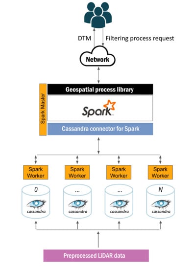
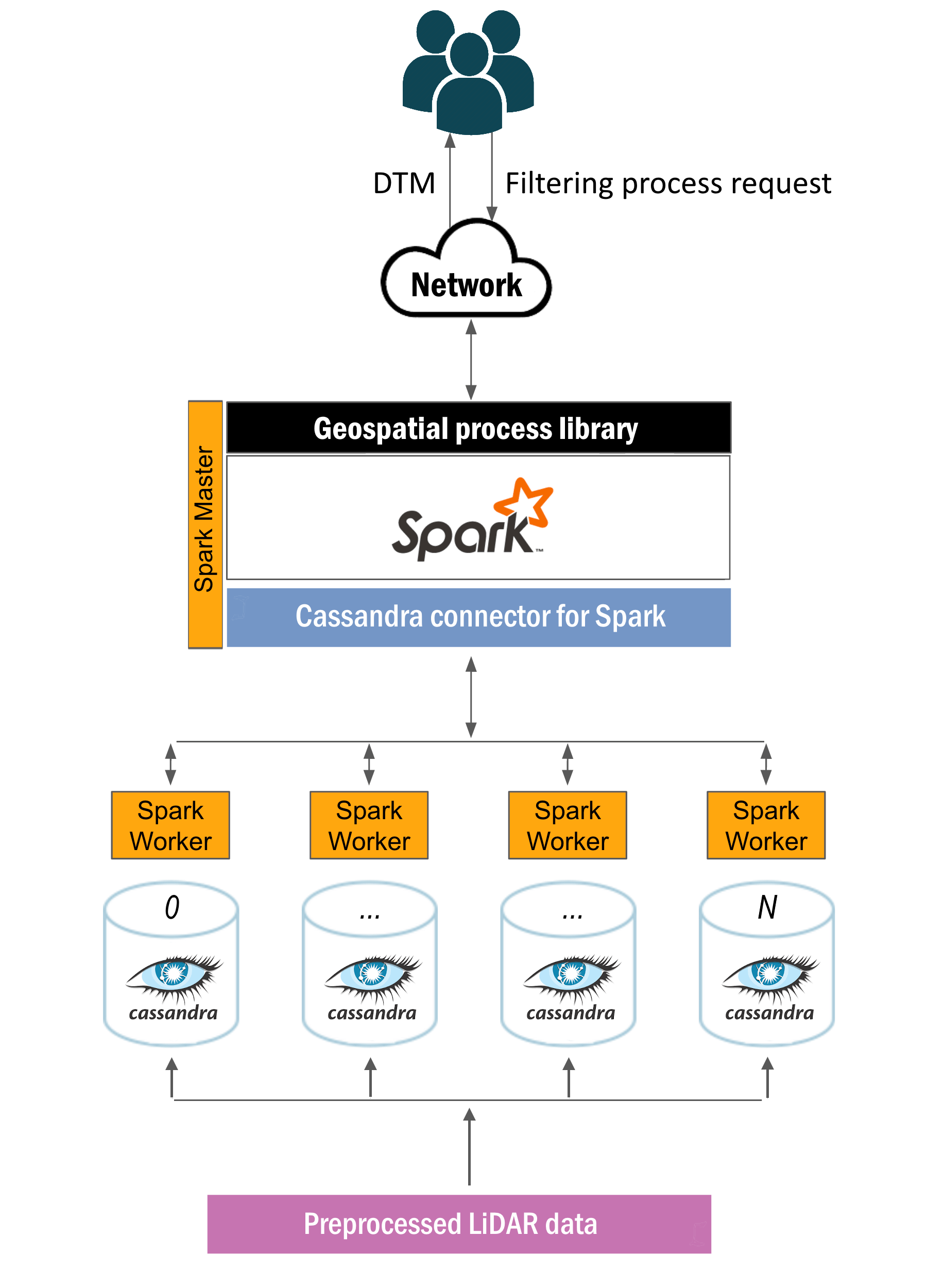
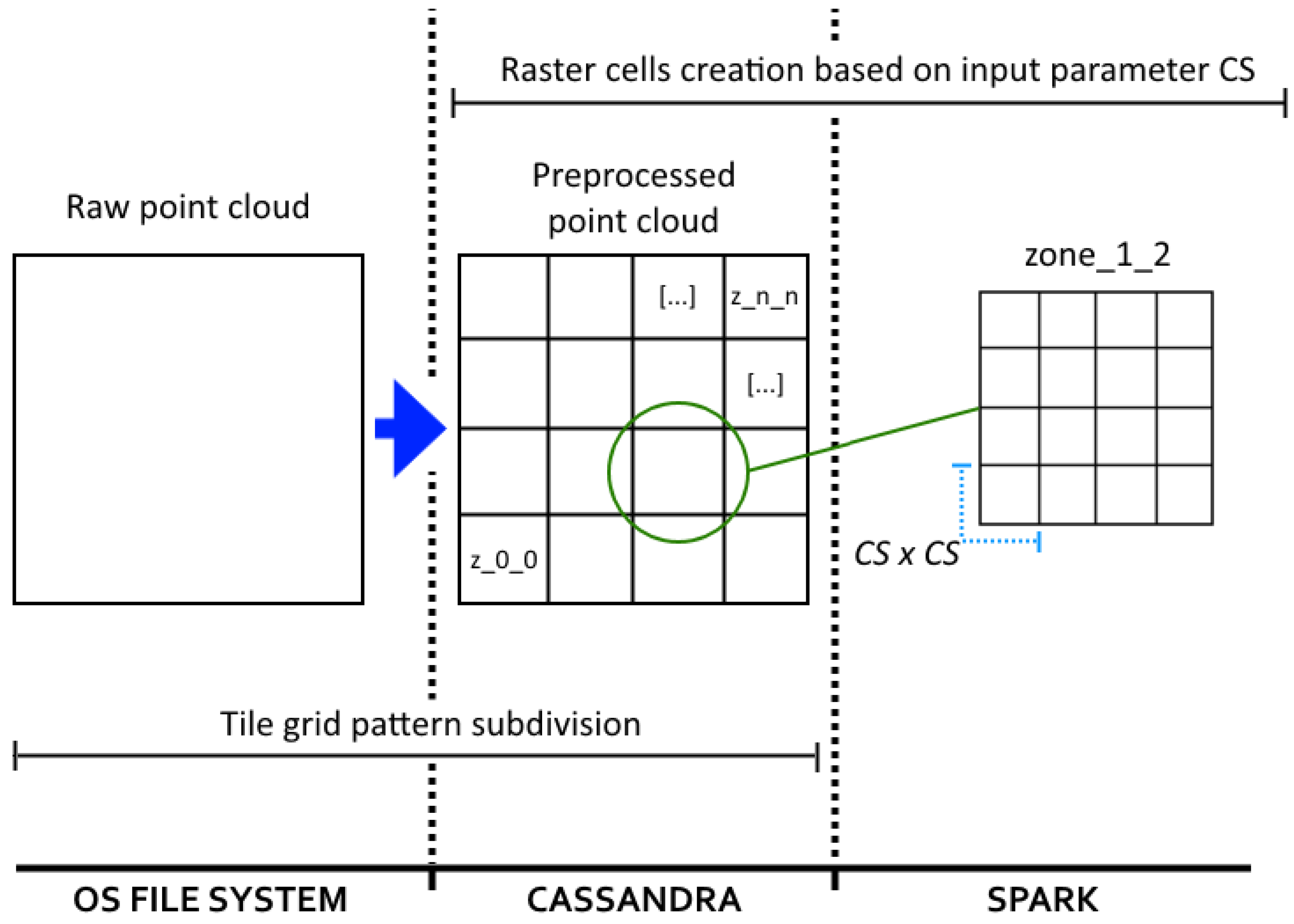
2.2. Distributed Storage: Cassandra

In [12], four of the most currently adopted and mature storage technologies were analyzed to determine the best option for the management of massive LiDAR datasets, as well as for supporting a web-based visualization framework. In the cited analysis, Hadoop Distributed File System (HDFS) [23], MongoDB [24], Cassandra [16] and Redis [25] were studied, attempting to include with each of them a different type of database design: distributed file systems, document stores, wide column stores and key-value stores [26]. Considering the conclusions of the aforementioned analysis, Cassandra was the storage technology selected for this work, since its querying capabilities are broad and very similar to those featured in other classic SQL (Structured Query Language) databases, and its integration with big data computing solutions, such as Spark, is efficient, stable and robust.

2.3. Distributed Computing: Spark

The system presented here can be considered as a batch processing system, since geospatial processes operate without supervision on well delimited large static LiDAR datasets. For such tasks, Spark stands out as the most suitable option thanks to its great integration with Cassandra through the Spark-Cassandra connector [27], as Java is one of its programming languages (same as the base source code of the filtering algorithm used), and owing to its design focused on batch processing and its operational versatility. Other popular computing solutions, such as Storm [28] and Flink [29], were discarded owing to their design focused more on streaming than on batch processing, while Hadoop [30] was discarded owing to its lack of programming models other than map-reduce.

Moving logic or algorithms between nodes is faster than moving data; this is one of the main principles of big data. Following this principle, maximum parallelism is ensured during the execution of the geospatial processes by deploying a Spark worker on each Cassandra cluster node. The Spark master distributes a copy of the geospatial process code (explained in Section 2.1) among the Spark workers so they can apply its computational tasks on subsets of LiDAR zones retrieved from Cassandra. The Spark–Cassandra connector ensures data locality, which means that each Spark worker only operates with the LiDAR zones stored on its own node, avoiding data movements between nodes. This is the general rule; nevertheless, it is not always followed or even desirable, as explained in the following sections. Pursuing the zone-level parallelism described in Section 2.1, each Spark worker operates only on its local subset of LiDAR zones, which are processed in parallel by being distributed among all physical cores available on each worker’s CPU.

Cassandra uses table keys to distribute data evenly throughout the nodes. The optimal performance of our application is achieved when the data distribution pattern matches the workload distribution pattern. If every node on the cluster stores the same percentage of the total data, and a geospatial process is executed using the whole data as input, every Spark worker will be assigned almost the same amount of workload. This is always the scenario during the analysis of Section 4. Workload distribution optimization [31] is beyond the scope of the research presented here.

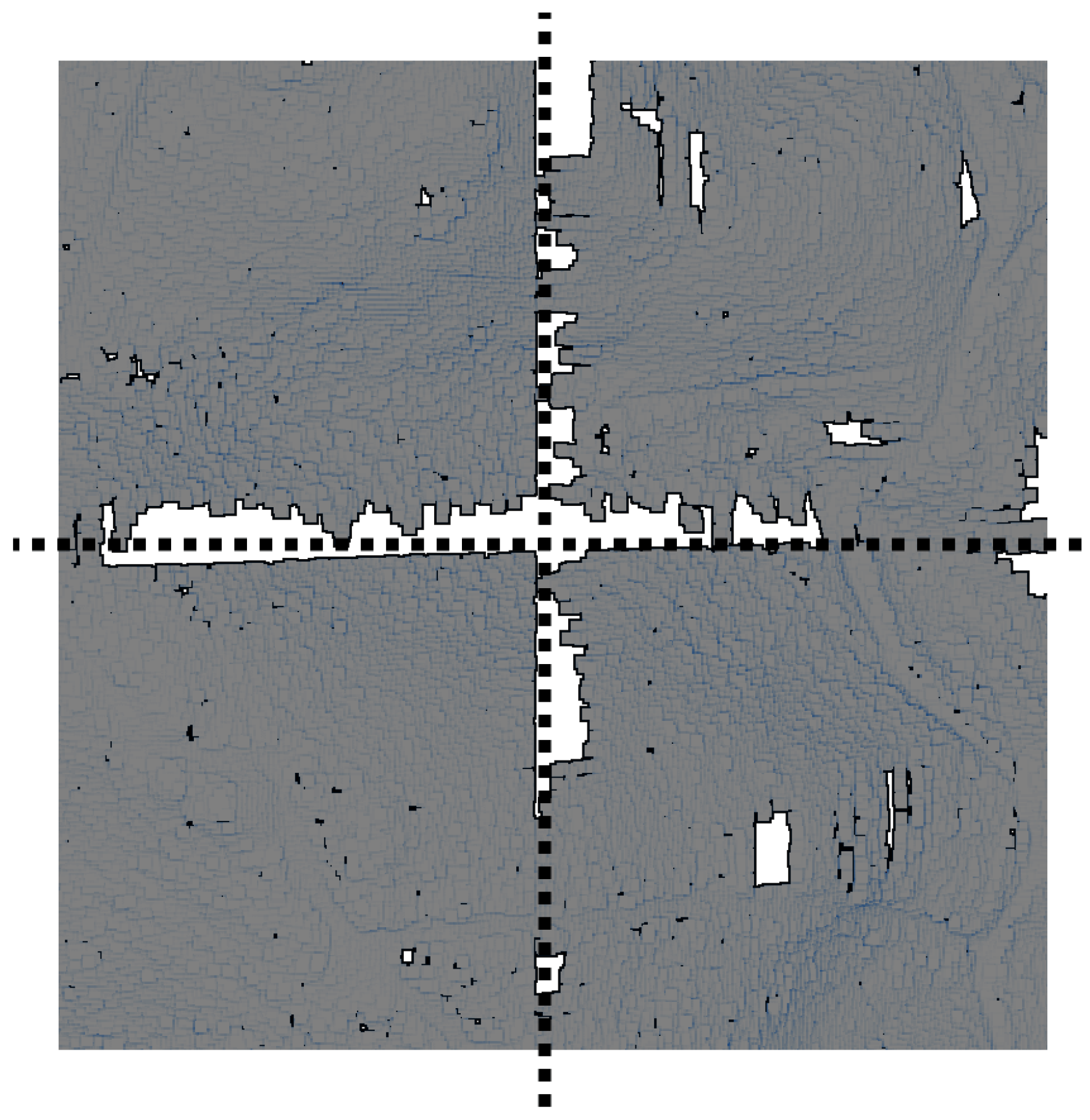
3. Automated Boundary Error Correction

The classification of a given point under the categories of ground or non-ground largely depends on the features of its neighboring points. Points located at the boundaries of adjacent zones filtered independently lack important information about their neighbors, thus it is very common to find classification errors at such locations. Figure 2 shows a raster of ground points obtained after filtering a point cloud that was subdivided into four zones during the preprocessing stage. Each zone was filtered independently from the rest and the classification results displayed together. As can clearly be seen, the final classification shows a regular pattern of gaps, far from being produced by natural geographic features or human-made structures, which match the boundaries of each zone. These gaps represent points that were misclassified as non-ground and thus do not appear on the image.

Usually, this type of errors is avoided through manual or semi-automatic (scripted) procedures. Users must firstly define overlapping sections between adjacent zones, then filter the zones together with the points from the overlapped sections, and finally crop the results to fit the original extent of each zone. In any case, this type of solutions always implies some kind of human intervention.

In this section, we present an automated error correction strategy which, taking advantage of the computational power of the big data system, automatically creates new additional overlapping rasters encompassing boundary sections between adjacent zones. The points from these overlapping rasters are also classified, obtaining as a result a collection of ground points that will be used to detect and correct the errors that may appear during the classification of the points of the zone rasters. For convenience, we call these collections correction patches. For example, in Figure 3, the squares outlined with continuous lines represent LiDAR zones, while the rectangles outlined with dots delimit the areas of the new overlapping rasters. The whole process is explained in the following subsections.

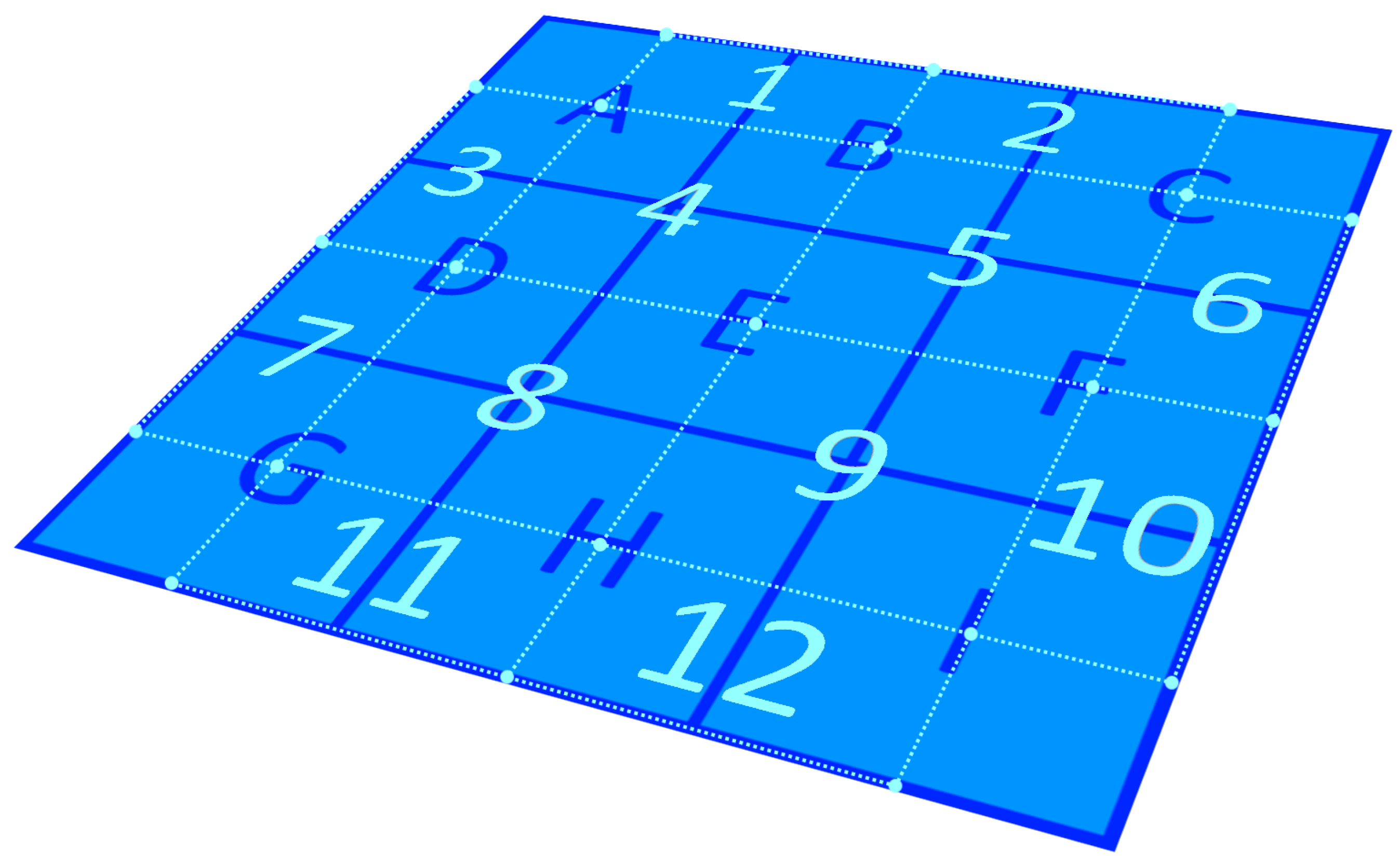
3.1. Creation of the Correction Patches

New overlapping rasters are created through a distributed process also carried out by the Spark + Cassandra system. Following the pattern depicted in Figure 3, a list with these new elements is made, taking into account all the LiDAR zones that are going to be filtered. Then, the elements of the list are evenly distributed throughout the Spark workers. Workers must retrieve from Cassandra all the necessary LiDAR zones to gather the points of each overlapping raster. For instance, to collect the points of the overlapping Raster 5 (see Figure 3), the worker in charge must request Zones B, C, E and F. In the same way as for the rasters of the zones, the input parameter $CS$ is used to define the cell dimensions on the overlapping rasters (see Figure 1).

Once the points of each overlapping raster have been gathered, the final correction patches are created by passing all those rasters to the classification process as input and obtaining as a result a collection of ground-only points for each one of them. The correction patches are stored temporally in Cassandra and deleted once the entire process is finished, since they are only valid for the specific input parameters used in the current classification process.

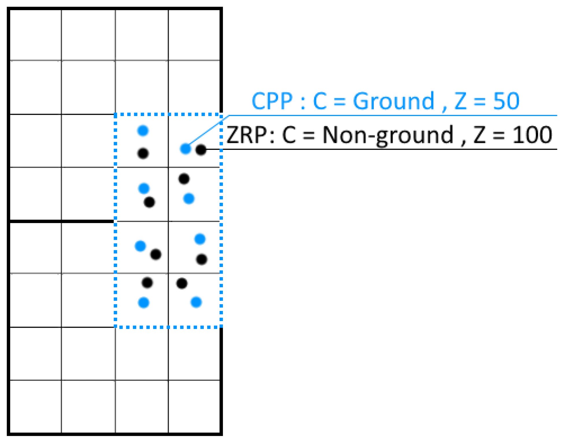
3.2. Filtering of the LiDAR Zones and Error Correction

All LiDAR zones are passed as input to the filtering algorithm. To ensure data locality, each Spark worker executes the algorithm over the zones stored in the same node it is deployed. A raster is created for each zone using $CS$ (as depicted in Figure 1) and then its points classified under the ground or non-ground categories. This output is a provisional classification, very likely to display errors on the boundary zones between zones.

After filtering a given LiDAR zone, each Spark worker retrieves from Cassandra the corresponding correction patches overlapping its surface. For instance, to correct the errors on the raster obtained from Zone H (see Figure 3), the worker in charge must request correction Patches 8, 9, 11 and 12. The information from the raster of the zone and the correction patches is combined to correct the errors found in the first one. Given two already classified points located at overlapping raster cells, one point taken from the raster of the LiDAR zone (zone–raster–point (ZRP)) and the other point taken from the correction patch (correction–patch–point (CPP)), the rules to correct the errors are defined as follows:

• If both points are labeled with the same class, the ZRP is considered as correctly classified, as was confirmed by the results of the patch.
• If a ZRP is classified as ground, but the CPP is classified as non-ground, the ZRP is considered as correctly classified. The overlapping rasters have their own boundary errors; if this scenario were considered as a classification error, the final results would display gaps that would match with the boundaries of the correction patches, thus, instead of correcting errors, new ones would be introduced.
• If a ZRP is classified as non-ground, but the CPP is classified as ground, the ZRP is considered as misclassified and ZRP should be labeled as ground. Additionally, following the same logic described in Section 2.1 for the selection of raster points, if the Z coordinate of ZRP is higher than the Z from CPP, the ZRP is replaced entirely by the CPP.

Figure 4 shows an example of the third case listed above. Squares outlined with an outer bold continuous line correspond to LiDAR zones, the vertical rectangle outlined with dots represents a correction patch and the remaining smaller squares are the raster cells from their corresponding rasters. In this example, an error is detected, as ZRP was classified as non-ground while CPP was classified as ground. The error is corrected by not only changing the class label of ZRP but replacing it entirely by CPP, since CPP has a lower Z value.

4. Results and Discussion

This section covers the analysis, in terms of executions times, on the performance and scalability of our proposal (Section 4.1), as well as a visual and quantitative analysis of the boundary error correction strategy (Section 4.2) and functional and computational considerations that should be highlighted regarding preprocessing decisions (Section 4.3) and full point classification (Section 4.4).

Two massive raw point clouds, whose details are described in

Table 1. Properties of the raw LiDAR point clouds selected for preprocessing. #P, Number of points (billions); #F, Number of files; FE, File extent (meters); FS, File size (average kilobytes per file); TS, Total point cloud size (GB).

Point Cloud	#P	#F	FE	FS	TS
PNOA (Region)	28	8697	2000 × 2000	96,731	802
Guitiriz (Village)	1	304	500 × 500	126,194	37

, were preprocessed to obtain the datasets employed for the analyses of this section. Four different datasets, whose details are described in

Table 2. Properties of the datasets used for the analysis. #Z, Number of zones; ZE, Zone extent (meters); ZS, Zone size (average kilobytes per zone); TS, Total dataset size (GB).

Dataset	Source	#Z	ZE	ZS	TS
D0	PNOA	11,662	1600 × 1600	8925	99
D1	PNOA	181,823	400 × 400	563	99
D2	PNOA	2,875,097	100 × 100	39	108
D3	Guitiriz	304	500 × 500	29,696	9

, were obtained out of the two raw point clouds. Datasets D0, D1 and D2 were created from the same point cloud (PNOA, see Figure 5a) varying the size of their processing units by using three different zone extents. On the other hand, D3 (created from the point cloud Guitiriz, see Figure 5b) was included to analyze system performance under especially unfavorable conditions, forcing the system to handle large processing units (29,690 KB per zone on average). During the preprocessing stage, not only was the subdivision of the point clouds carried out, but also a compression of the resultant files. A compression method, very similar to the one described in [3], was employed to reduce the size of the data to be handled by the system.

All machines used on the system deployment follow the same specifications: 2×Intel Xeon E5-2660 (16 Cores/32 Threads), 64 GB RAM (DDR3), SATA3 HDD (7.2k), CentOS (6.10) and InfiniBand connection. The Spark master runs along with a Spark worker and a Cassandra node due to the negligible workload on the master. Both Spark and Cassandra offer a large number of configurable settings. To obtain the best performance results, these settings must be configured taking into account the cluster topology and the nature of the algorithms executed as well as the amount and type of data involved. The most relevant settings configured are described in Appendix A. The filtering algorithm was configured with the input parameters described in Section 2.1, setting $CS$ to 1.5 following recommendations from Recarey et al. [22].

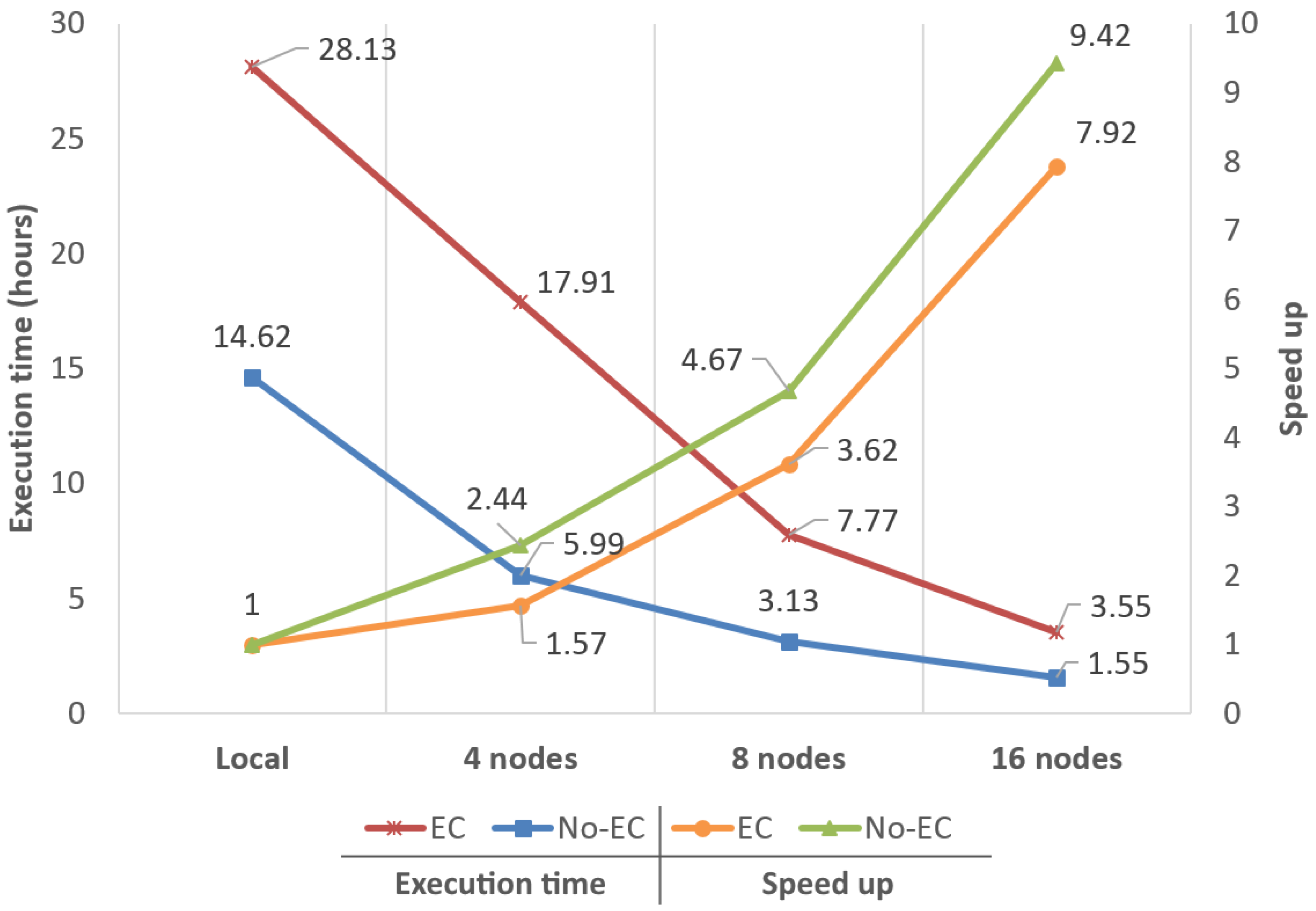
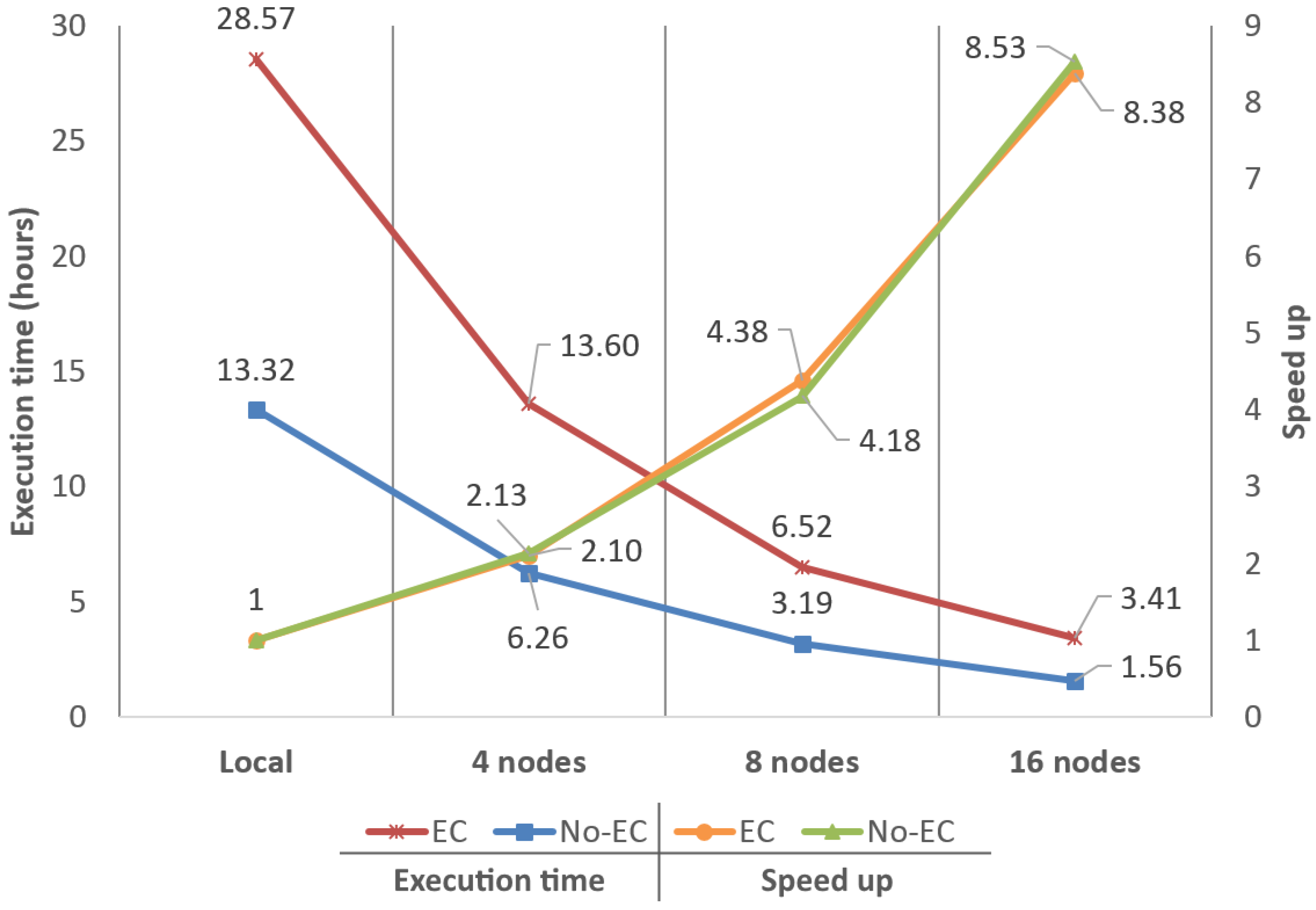
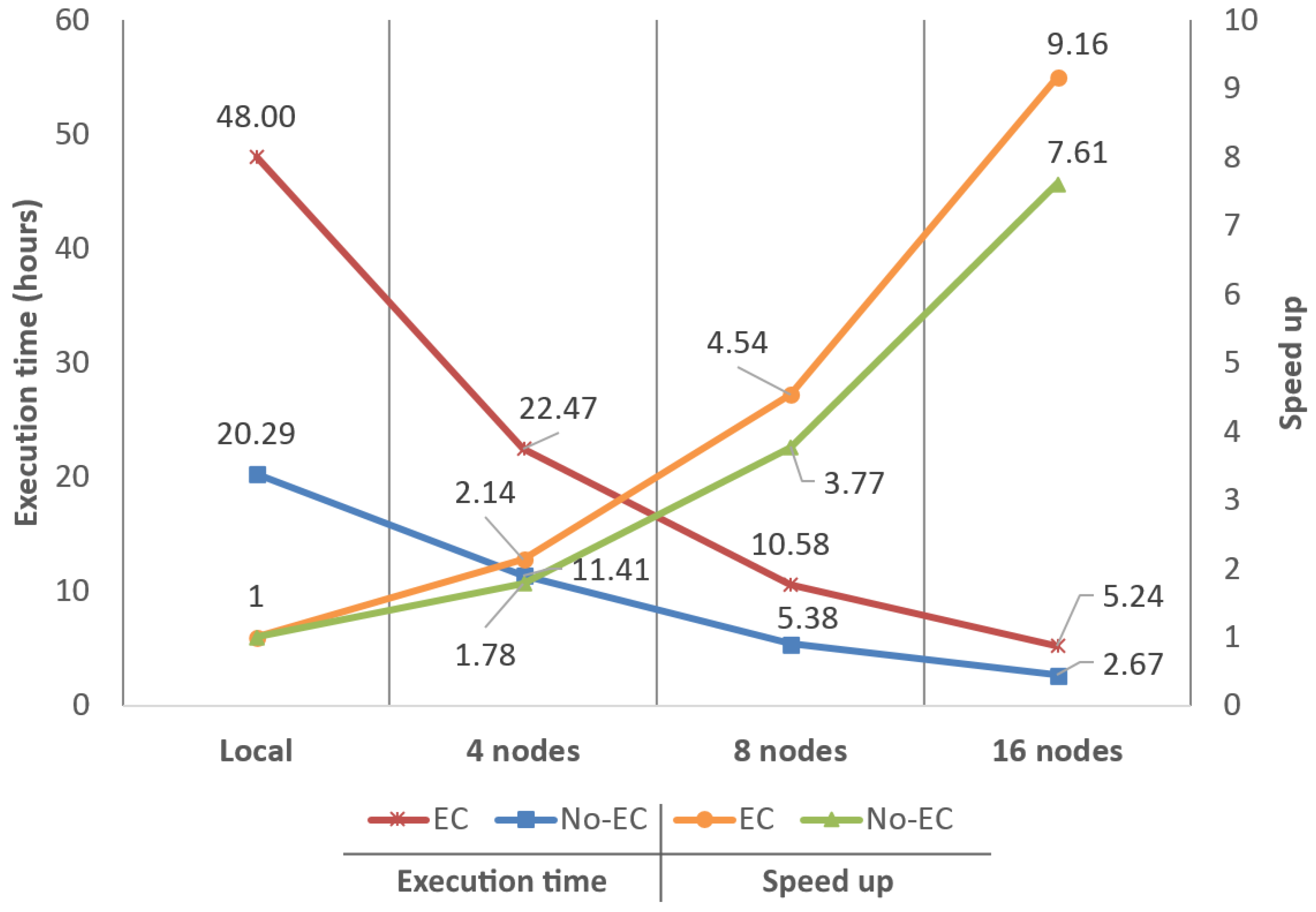
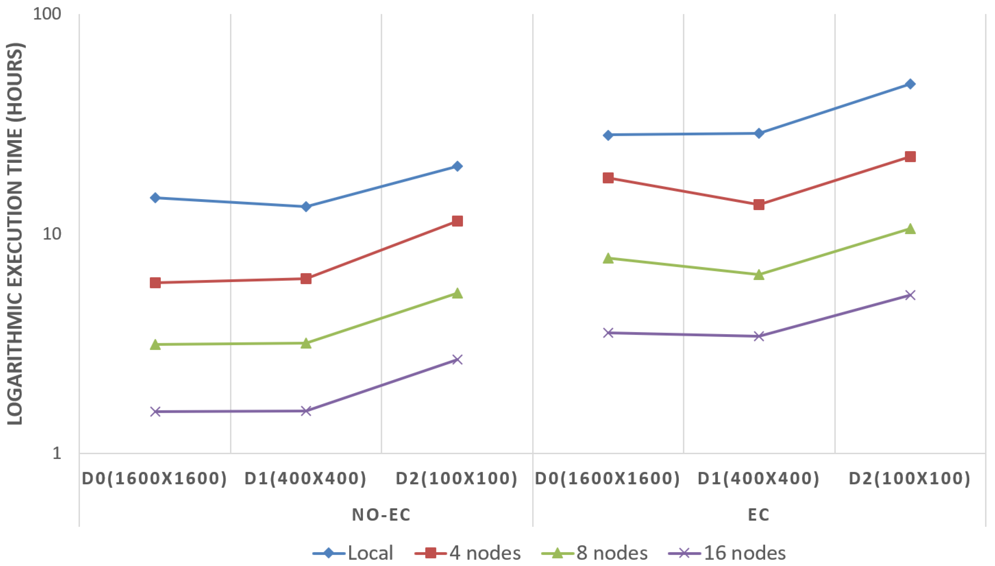
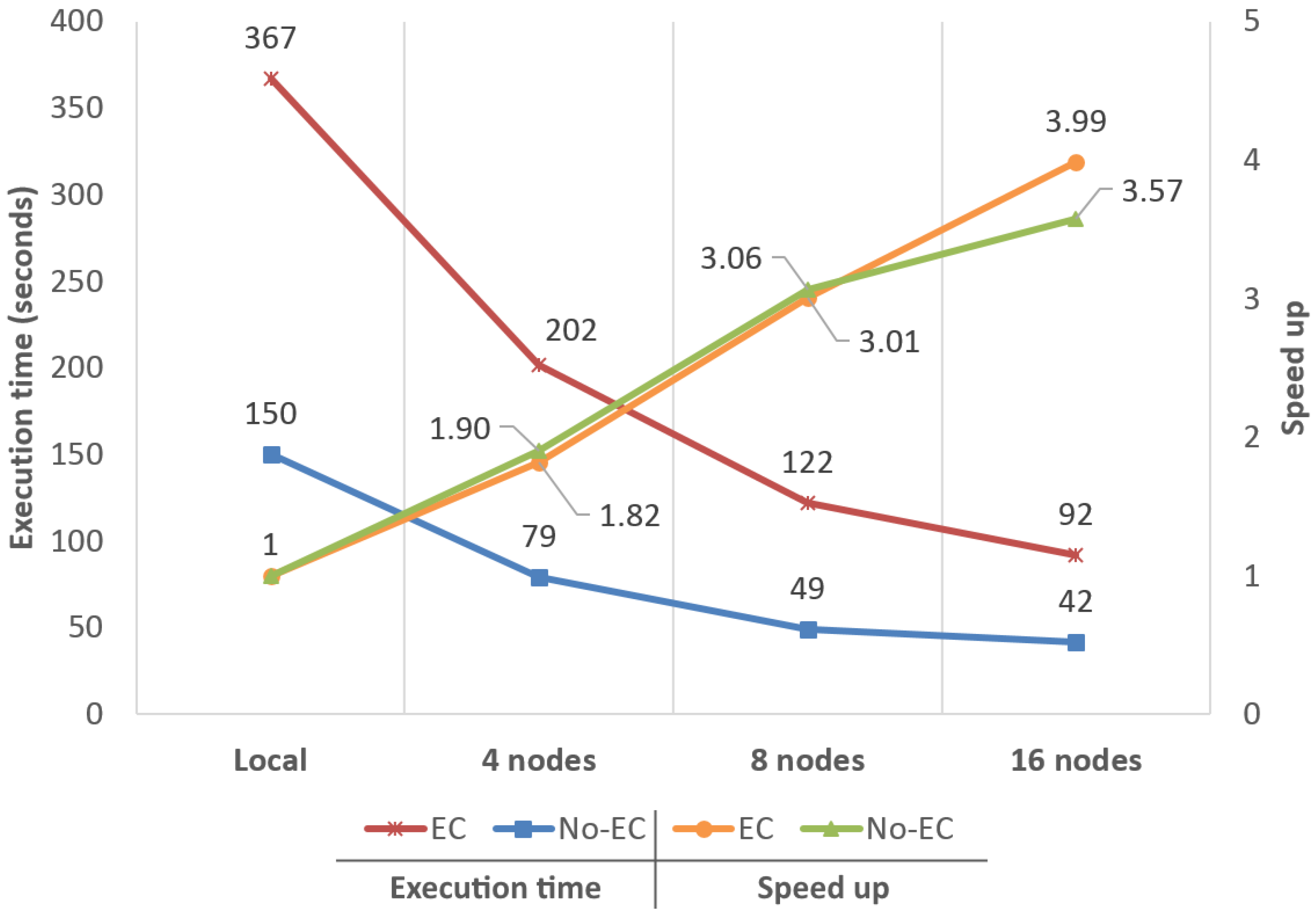
4.1. Performance in Terms of Execution Times

To analyze the scalability and performance of the system, we measured the time it took to filter each of the four datasets described in Table 2. We should remember here that the whole filtering process encompasses the creation of the rasters, the classification of the points from the rasters and, if selected, the error correction. Times were taken for two execution scenarios: one using the error correction strategy (EC) and the other one without using it (NO-EC). The analysis was carried out using 4, 8 and 16 computing nodes. As a base comparison, a local non-big-data version of the system was also tested. This local version was specially configured to run in one node, without using Cassandra or Spark, being capable of processing in parallel several zones by sharing the workload among the 16 local nodes.

Performance results for D0, D1 and D2 can be observed in Figure 6, Figure 7 and Figure 8, respectively. Figures show execution times (in hours) and speed-ups in comparison to the reference value (the local version of the algorithm).

Regarding speed-ups, results obtained for D0 were $1.57\times$, $3.62\times$ and $7.92\times$ with EC and $2.44\times$, $4.67\times$ and $9.42\times$ with NO-EC (using 4, 8 and 16 nodes, respectively). For D1, speed-ups observed were almost the same in both execution scenarios, being around $2.1\times$, $4.2\times$ and $8.4\times$. Finally, for D2, speed-ups were $2.14\times$, $4.54\times$ and $9.16\times$ with EC and $1.78\times$, $3.77\times$ and $7.61\times$ with NO-EC. Considering these results, it can be asserted that the base speed-up obtained when moving from a local execution to the big data system using four nodes is, on average, $2\times$. Hence, the big data system shows linear scalability for all node configurations and datasets, both with EC and NO-EC, by doubling the performance when doubling the nodes available.

Regarding execution times, the fastest configuration observed offering the best quality was the 16 nodes configuration with EC and zones of $400\times 400$ (D1) achieving 3.41 h. Presumably, execution times observed for D2 should be always better than D1, and times observed for D1 better than D0, since a reduction in the KB per zone would improve the throughput and latency of Cassandra, as demonstrated in [12]. However, in this comparison, the effects on the reduction in the extent of the zones showed very different results. These differences are explained by the variation on the amount of information that moves between nodes in the two different execution scenarios and the start-up/initialization time penalty of the filtering algorithm. Every time a given processing unit (zone) begins to be filtered, a certain number of data structures must be initialized and some initial computations must be made causing a small start-up/initialization time penalty; hence, the more zones that are filtered, the more start-up/initialization time penalties will occur.

In the first scenario (NO-EC), data movements between nodes are almost non-existent as the Spark–Cassandra connector ensures data locality. Spark workers only apply the filtering algorithm on the zones stored in their own nodes and, as a result, little to no reduction on execution times is obtained by reducing the KB per zone. On the other hand, the start-up penalty of the filtering algorithm increases along with the number of zones to be processed. As a result of the combination of these two performance issues, in this scenario, a reduction in the extent of the zones is very likely to always produce an increment in the execution times.

In the second scenario (EC), there are considerably more data movements between nodes; for example, a given correction patch should be moved between nodes for correcting the errors of adjacent zones that were stored in different nodes. Once the number of data movements is significant enough, the potential performance gain related to the reduction of the KB per zone begins to show up. The time reduction related to the movement of the data between nodes may end up compensating the time increment related to the start-up penalties, producing an overall decrement in the execution times.

Figure 9 shows (using a logarithmic scale) how the execution times vary when changing the extent of the zones with NO-EC and EC. It can be clearly seen how there is always a reduction in the execution times when increasing the extent of the zones from $100\times 100$ to $400\times 400$. The reduction in the number of zones to be filtered causes an important improvement in the execution times observed, which helps to compensate the potential performance decrement produced by the increase in the number of bytes that must be moved throughout the system when the boundary errors are corrected. However, when going from $400\times 400$ to $1600\times 1600$, execution times almost stall. There is no a significant improvement with NO-EC; thereby, when the boundary errors are corrected, the amount of data becomes high enough to cause decrement in the performance of the system, leading to the obtention of worse times with EC.

Finally, speed-ups obtained for D3 (Figure 10) were $1.9\times$, $3.06\times$ and $3.57\times$ for NO-EC and $1.82\times$, $3.01\times$ and $3.99\times$ for EC. As can be observed, although the performance boost of the big data approach was notable, in comparison, results were not as good as those obtained with the other datasets, even starting to stall just at $\approx 4\times$ when running on 16 nodes. These results are explained by, not only the small number of zones to process in comparison to the available cores (1.19 zones per core), but also by the very large size of the zones (≈ 30 MBs) that are being processed.

4.2. Boundary Error Correction Quality

With the intention of analyzing our boundary error correction strategy, we employed three separate methods: a visual analysis using the massive dataset D3 and two quantitative analyses using some of the datasets provided by the International Society for Photogrammetry and Remote Sensing (ISPRS) [32].

Visual comparisons between EC and NO-EC can be observed in Figure 11 and Figure 12. Images in Figure 11 show a close view over two filtered rasters from D3 containing ground points only. The surface shown in Figure 11a presents noticeable errors with blank zones that are completely removed in Figure 11b. The only blank zones that can be seen in this image correspond to large zones of forest or small groups of houses. On the other hand, Figure 12 shows an even closer view over two fully triangulated rasters from the previous raster set. Ground points from the rasters were triangulated using the software tool Global Mapper [33]. As in the previous figure, clear errors can be observed in Figure 12a along the boundaries of the zones, while they are completely absent in Figure 12b.

In

Table 3. Type I error comparison (lower is better) between EC and NO-EC using some of the datasets provided by the ISPRS [32].

Datasets	Type I Error (%)
	Undivided	Divided in 4 (NO-EC)	Divided in 4 (EC)
Sample 11	45.99	50.18	44.97
Sample 22	39.71	40.59	39.44
Sample 52	10.79	13.43	10.54
Sample 53	14.87	15.71	14.25
Sample 54	6.80	7.22	6.47
Sample 61	8.03	8.44	7.76

, we present a quantitative comparison between EC and NO-EC using the standard Type I error (rejection of ground points). We should stress here that Type I errors are calculated only with points from the rasters, thus every point from a raw point cloud not included in a raster counts as a classification error, leading to the high percentages shown in the table. The comparison was carried out using several datasets taken from the ISPRS test sites (first column) since they are considered as a standard when it comes to testing classification algorithms. For these tests, $CS$ was set to 1 due to the low point density of the datasets. The second column (Undivided) shows the Type I errors obtained for each dataset using as input the entire undivided point clouds. All datasets were also divided into four smaller and equally sized zones (using the same division pattern shown in Figure 2), and then each zone was processed with NO-EC and EC (third and fourth columns).

By dividing the datasets, boundary errors appear between the four zones, as can be observed by comparing the second and third columns of Table 3. While comparing the third and fourth columns, the percentage of errors is reduced beyond the level previous to the division of the datasets thanks to the use of our proposal. The percentage of errors observed with EC are slightly inferior to the percentage with the undivided datasets, which can be explained by two main reasons. The first is due to small numbers of extra points that can be contained in the rasters of the divided datasets. For example, considering a raster created from a zone of 9 m × 9 m and using $CS$ = 1 m, the resultant raster will contain 81 points distributed in a grid of 9 × 9 cells. After dividing the zone into four smaller areas of 4.5 m × 4.5 m, the four resultant rasters will contain 100 points distributed in four grids of 5 × 5 cells, since those half meters remaining imply the presence of an additional cell on each grid dimension. This extra information helps to improve the quality of the classification reducing and, as a result, the Type I errors. The second reason is due to the surface of the correction patches, which can extend beyond the boundaries of the zones and, therefore, some misclassified points located away from the boundaries could also be corrected during the process.

To measure the misclassification of points due to the divisions on the datasets and the improvement of our automated boundary error correction strategy, a new metric is proposed:

$$\delta ={\displaystyle \frac{{(\mathsf{\#}GP-\mathsf{\#}MP)}_{divided}}{{(\mathsf{\#}GP-\mathsf{\#}MP)}_{undivided}}}\times 100$$

(1)

where $\mathsf{\#}GP$ stands for the number of ground points (total) and $\mathsf{\#}MP$ for the number of misclassified ground points.

Table 4. Misclassification of points due to the divisions on the datasets and the improvements of our proposal using some of the datasets provided by the ISPRS [32]. Variations in classification quality are measured with the $\delta$ metric (higher is better).

Datasets info.		Rasters info.
				Undivided		Divided in 4 (NO-EC)			Divided in 4 (EC)
Name	#GP	#GP	#MP	#GP	#MP	$\delta$ (%)	#GP	#MP	$\delta$ (%)
Sample 11	21,781	12,218	453	11,416	414	93.51	12,599	566	102.28
Sample 22	22,498	13,843	280	13,769	400	98.57	14,101	468	100.52
Sample 52	20,112	18,119	177	17,532	180	96.71	18,104	186	99.87
Sample 53	32,989	28,208	124	27,875	124	98.81	28,349	124	100.50
Sample 54	3983	3866	154	3845	154	99.43	3877	160	100.13
Sample 61	33,854	31,195	59	31,045	57	99.52	31,284	60	100.28

shows the new metric described above using some of the datasets from the ISPRS. The first two columns provide information about the original ISPRS datasets, while the other columns display information about the obtained rasters and the new metric.

As can be clearly seen, after dividing the original datasets $\delta <100$ for all rasters with NO-EC, since many ground points correctly classified in the undivided rasters, they are no longer presented in the divided ones. With EC, many of the correctly classified ground points lost after the divisions are restored, obtaining $\delta \ge 100$. It should be noted here that in most cases $\delta >100$ due to small numbers of extra points that are included to the raster with our error correction strategy.

4.3. The Importance of an Adequate Point Cloud Preprocessing

All results presented in Section 4.1 and Section 4.2 reveal the great importance of the decisions taken during the preprocessing stages of the LiDAR datasets, since how point clouds are divided and stored in Cassandra will largely determine the system performance.

Reducing the byte size of the zones by reducing their extent may improve the overall system performance; nevertheless, once a certain extent is reached, the performance improvement may get stuck or even get worse (as explained in Figure 9).

With a significant volume of data movements between the nodes, Cassandra will tend to perform better the smaller (in bytes) the zones are. However, this volume of data will be largely determined by the type of geospatial processes running on the system and how they have been programmed to run in Spark. While it may seem obvious at first that the optimal way to proceed during the preprocessing stages is to divide the point clouds into zones as small as possible, with such decision, we could be increasing the workload of Spark, for example, in the use case presented in this work, by having to correct all boundary errors produced by the divisions in the point clouds (as shown in Table 3).

Owing to this, when deciding how point clouds will be divided and stored, not only the number of data movements between nodes should be considered, but also whether the output quality of the algorithms running in Spark is related to the byte size or extent of the zones and how said features can affect the workload and performance of Spark.

By way of conclusion, it should be stressed how critical it is to find a suitable balance between the number of zones (#Z), the size per zone (ZS) and the output quality of the geospatial process. Developing an automated method to determine the optimal number of zones, or their extent, is beyond the scope of this work, but it would be considered as an interesting part of the future work.

4.4. Full Point Classification

It is intended to expand the type of output of the current filtering algorithm with the goal of offering full point classification. We have developed a naive approach to analyze the potential of this additional feature. To accomplish this task, the current filter output is used as input for a new final stage to classify all the points in the raw point cloud. Based on their X and Y coordinates, each point from the LiDAR zones is placed in a cell from the already filtered rasters. If the height difference between the point located in the raster cell and the point from the zone is less than an customizable parameter, which we have called height threshold ($HT$), the new unclassified point is labeled using the same class as the raster point; otherwise, the point is labeled with the opposite class.

Table 5. A comparison between the full point cloud classification errors (lower is better) obtained by the naive method proposed and LAStools.

Datasets	Total Error (%)		Type I Error (%)		Type II Error (%)
	Our Approach	LAStools	Our Approach	LAStools	Our Approach	LAStools
Sample 11	17.05	17.67	27.06	26.94	3.61	5.18
Sample 12	5.28	6.97	8.25	12.87	2.16	0.77
Sample 21	1.79	6.66	1.42	7.98	3.09	1.87
Sample 53	14.33	14.37	14.55	14.84	8.92	3.24
Sample 61	7.29	17.24	7.38	17.85	4.89	0.40
Average	9.15	12.58	11.732	16.10	4.53	2.29

shows a comparison between this naive approach and LAStools [34] using the ISPRS Filter Test datasets. The LAStools results were obtained from [35], as it is one of the latest research articles about ground classification from LiDAR point clouds. The analysis was carried out comparing Total errors (percentage of misclassified points), Type I errors (rejection of ground points) and Type II errors (acceptance of non-ground points as ground points). The $CS$ parameter was set to 1, again due to the low point density of the datasets, while the $HT$ parameter was set to 30 cm.

The results obtained show how our approach is better, on average, than LAStools when considering the Total errors and the Type I errors, but slightly worse when considering Type II errors, which is an expected result, since the core design of the SC-091-12 algorithm was focused on the obtention of rasters with ground points and not on the identification of non-ground points. Among all the samples provided by ISPRS, Sample 11 is known to be one of the most difficult when it comes to being processed by the different classification algorithms, mainly due to the high degree of slope of the terrain together with the large number of structures covering its entire surface. As mentioned above, in this first approach to the full classification of point clouds, we have implemented a naive method of classification, which, for the specific case of Sample 11, obtains a greater number of Type I errors than those obtained for the rest of the samples; nonetheless, it offers a percentage of error almost identical to that obtained by LAStools. The inclusion of the full point classification has been established as future work, as well as the reduction in the error rates.

5. Conclusions and Future Work

In this work, we have proven how big data technologies, in this case Cassandra and Spark, provide very powerful solutions for the large-scale parallelization of geospatial processes. The distributed computing system presented in this work allowed us to greatly improve the performance of the SC-091-12 algorithm. In addition to the outstanding computing capacity of these two technologies working together, their highly programmable design provides the opportunity to further improve and expand the functionality of the geospatial processes through the easy inclusion of new computational stages, such as the error correction stage also introduced here. Said strategy allowed us to correct the classification errors that can be found on the boundaries of adjacent zones independently processed by the filtering algorithm.

Performance results obtained show how our proposal was capable of reducing the time it took to process 28 billion points in a single machine, from 28.57 to 3.41 h when correcting the boundary errors, and from 13.32 to 1.56 h with no error correction, obtaining a speed-up of $8.4\times$ for deployments of 16 nodes (see Figure 7). The use of a big data approach brings not only distributed computing to LiDAR data, but also all the common storage advantages associated to this type of technologies, such as high data availability and scalability or fault tolerance. GIS centers, governmental institutions or any other kind of group working with very large volumes of data will greatly benefit from the proposal presented here and, with the appropriate amount of computational resources, the entire process of obtaining fully triangulated DTMs could get near to real-time processing.

As future work, we are heading towards finishing the full classification of point clouds using a more refined and complex algorithm than the one presented in Section 4.4 so the system can be configured to obtain just a filtered raster from a given point cloud or the whole filtered point cloud. Additionally, the development of an automated method to determine the optimal number and extent of the processing units could be considered for minimizing the human intervention while maximizing the performance of the distributed computed system.

The autonomous nature of all computing stages, along with the low processing times achieved, opens up the possibility of considering the system as a service-oriented solution for on-demand DTM/DSM generation, which would be a highly useful and unique service for many users in the LiDAR field, and one which could get near to real-time processing with appropriate computational resources. The distributed computed system presented in this work serves as base system to a larger one offering several geospatial processes in the form of a library of geospatial processes, with the aim of applying those process over entire point clouds or only regions of interest defined by the users.

References

1. González-Ferreiro, E.; Miranda, D.; Barreiro-Fernández, L.; Buján, S.; García-Gutiérrez, J.; Diéguez-Aranda, U. Modelling stand biomass fractions in Galician Eucalyptus globulus plantations by use of different LiDAR pulse densities. For. Syst. 2013, 22, 510–525. [Google Scholar] [CrossRef]
2. Ventura, G.; Vilardo, G.; Terranova, C.; Sessa, E.B. Tracking and evolution of complex active landslides by multi-temporal airborne LiDAR data: The Montaguto landslide (Southern Italy). Remote Sens. Environ. 2011, 115, 3237–3248. [Google Scholar] [CrossRef]
3. Deibe, D.; Amor, M.; Doallo, R. Supporting multi-resolution out-of-core rendering of massive LiDAR point clouds through non-redundant data structures. Int. J. Geogr. Inf. Sci. 2019, 33, 593–617. [Google Scholar] [CrossRef]
4. Rodríguez, M.B.; Gobbetti, E.; Marton, F.; Tinti, A. Coarse-grained Multiresolution Structures for Mobile Exploration of Gigantic Surface Models. In Proceedings of the SIGGRAPH Asia 2013 Symposium on Mobile Graphics and Interactive Applications, Hong Kong, China, 19–22 November 2013. [Google Scholar]
5. Hashem, I.A.T.; Yaqoob, I.; Anuar, N.B.; Mokhtar, S.; Gani, A.; Khan, S.U. The rise of big data on cloud computing: Review and open research issues. Inf. Syst. 2015, 47, 98–115. [Google Scholar] [CrossRef]
6. Yang, C.; Yu, M.; Hu, F.; Jiang, Y.; Li, Y. Utilizing Cloud Computing to address big geospatial data challenges. Comput. Environ. Urban Syst. 2017, 61, 120–128. [Google Scholar] [CrossRef] [Green Version]
7. Li, S.; Dragicevic, S.; Castro, F.A.; Sester, M.; Winter, S.; Coltekin, A.; Pettit, C.; Jiang, B.; Haworth, J.; Stein, A.; et al. Geospatial big data handling theory and methods: A review and research challenges. Isprs J. Photogramm. Remote Sens. 2016, 115, 119–133. [Google Scholar] [CrossRef] [Green Version]
8. Wang, L.; Ma, Y.; Yan, J.; Chang, V.; Zomaya, A.Y. pipsCloud: High performance cloud computing for remote sensing big data management and processing. Future Gener. Comput. Syst. 2018, 78, 353–368. [Google Scholar] [CrossRef] [Green Version]
9. Ma, Y.; Wu, H.; Wang, L.; Huang, B.; Ranjan, R.; Zomaya, A.; Jie, W. Remote sensing big data computing: Challenges and opportunities. Future Gener. Comput. Syst. 2015, 51, 47–60. [Google Scholar] [CrossRef]
10. Boehm, J. File-centric Organization of large LiDAR Point Clouds in a Big Data context. In Proceedings of the IQmulus First Workshop on Processing Large Geospatial Data, Cardiff, UK, 8 July 2014; pp. 69–76. [Google Scholar]
11. Brédif, M.; Vallet, B.; Ferrand, B. Distributed Dimensonality-Based Rendering of Lidar Point Clouds. Isprs - Int. Arch. Photogramm. Remote Sens. Spat. Inf. Sci. 2015, XL-3/W3, 559–564. [Google Scholar]
12. Deibe, D.; Amor, M.; Doallo, R. Big data storage technologies: A case study for web-based LiDAR visualization. In Proceedings of the 2018 IEEE International Conference on Big Data (Big Data), Seattle, WA, USA, 10–13 December 2018; pp. 3831–3840. [Google Scholar]
13. Persson, H.; Wallerman, J.; Olsson, H.; Fransson, J.E. Estimating forest biomass and height using optical stereo satellite data and a DTM from laser scanning data. Can. J. Remote Sens. 2013, 39, 251–262. [Google Scholar] [CrossRef]
14. Zhou, X.; Li, W.; Arundel, S.T. A spatio-contextual probabilistic model for extracting linear features in hilly terrains from high-resolution DEM data. Int. J. Geogr. Inf. Sci. 2019, 33, 666–686. [Google Scholar] [CrossRef]
15. Deibe, D.; Amor, M.; Doallo, R.; Miranda, D.; Cordero, M. GVLiDAR: An Interactive Web-based Visualization Framework to Support Geospatial Measures on Lidar Data. Int. J. Remote Sens. 2017, 38, 827–849. [Google Scholar] [CrossRef]
16. The Apache Software Foundation. Apache Cassandra. Available online: http://cassandra.apache.org/ (accessed on 8 January 2018).
17. The Apache Software Foundation. Apache Spark. Available online: http://spark.apache.org/ (accessed on 22 January 2019).
18. Buyya, R.; Dastjerdi, A.; Calheiros, R. Big Data Principles and Paradigms; Elsevier Science: Amsterdam, The Netherlands, 2016; pp. 39–58. [Google Scholar]
19. Zhang, K.; Chen, S.C.; Whitman, D.; Shyu, M.L.; Yan, J.; Zhang, C. A progressive morphological filter for removing nonground measurements from airborne LIDAR data. IEEE Trans. Geosci. Remote Sens. 2003, 41, 872–882. [Google Scholar] [CrossRef] [Green Version]
20. Crecente, R.; González, E.; Arias, D.; Miranda, D.; Suárez, M. LIDAR2MDTPlus Generación de Modelos Digitales de Terreno de Pendiente Variable a Partir de datos LIDAR Mediante Filtro Morfológico Adaptativo y Computación Paralela Sobre Procesadores Multinúcleo, 2012. Software registration: Universidade de Santiago, Spain. SC-091-12 03/28/2012. Available online: http://www.ibader.gal/seccion/378/Outras-actividades.html (accessed on 21 February 2020).
21. USDA Forest Service. FUSION/LDV LIDAR Analysis and Visualization Software. Available online: http://forsys.cfr.washington.edu/fusion/fusion_overview.html (accessed on 22 January 2019).
22. Recarey, V.C.; Barrós, D.M.; Prado, D.A.A. Optimización de los Parámteros del Algoritmo de Filtrado LiDAR2MDTPlus, Para la Obtención de Modelos Digitales del Terreno con LiDAR. Ph.D. Thesis, Higher Polytechnic Engineering School, University of Santiago de Compostela (USC), Santiago de Compostela, Spain, September 2014. [Google Scholar]
23. The Apache Software Foundation. Apache Hadoop 3.0.0—HDFS Architecture. Available online: http://hadoop.apache.org/docs/r3.0.0/hadoop-project-dist/hadoop-hdfs/HdfsDesign.html (accessed on 8 January 2018).
24. MongoDB, Inc. MongoDB. Available online: http://www.mongodb.com/ (accessed on 8 January 2018).
25. Redis Labs. Redis. Available online: http://redis.io/ (accessed on 8 January 2018).
26. solid IT. DB-Engines Ranking—Popularity Ranking of Database Management Systems. Available online: http://db-engines.com/en/ranking (accessed on 8 January 2018).
27. Datastax. GitHub—Datastax/spark-Cassandra-Connector: DataStax Spark Cassandra Connector. Available online: https://github.com/datastax/spark-cassandra-connector (accessed on 22 January 2019).
28. The Apache Software Foundation. Apache Storm. Available online: http://storm.apache.org/ (accessed on 11 March 2019).
29. The Apache Software Foundation. Apache Flink: Stateful Computations over Data Streams. Available online: https://flink.apache.org/ (accessed on 11 March 2019).
30. The Apache Software Foundation. Apache Hadoop. Available online: http://hadoop.apache.org/ (accessed on 11 March 2019).
31. Lin, S.; Chen, H.; Hu, F. A Workload-Driven Approach to Dynamic Data Balancing in MongoDB. In Proceedings of the 2015 IEEE International Conference on Smart City/SocialCom/SustainCom (SmartCity), Chengdu, China, 19–21 December 2015; pp. 786–791. [Google Scholar]
32. University of Twente. ISPRS Test Sites. Available online: https://www.itc.nl/isprs/wgIII-3/filtertest/downloadsites (accessed on 27 April 2019).
33. Blue Marble Geographics. Global Mapper—All-in-one GIS Software. Available online: https://www.bluemarblegeo.com/products/global-mapper.php (accessed on 10 May 2019).
34. GmbH, R. LAStools. Available online: https://rapidlasso.com/lastools/ (accessed on 15 May 2019).
35. Rizaldi, A.; Persello, C.; Gevaert, C.; Oude Elberink, S. Fully Convolutional Networks for Ground Classification from LiDAR Point Clouds. Isprs Ann. Photogramm. Remote Sens. Spat. Inf. Sci. 2018, 4, 231–238. [Google Scholar] [CrossRef] [Green Version]
36. Universidade de Santiago de Compostela (USC). Laboratorio do Territorio (Laborate). Available online: http://laborate.usc.es/index.html (accessed on 23 October 2018).
37. Infraestructura de Datos Espaciales de España (IDEE). Geoportal IDEE. Available online: http://www.idee.es/ (accessed on 8 March 2019).
Figure 1. Data divisions carried out during the whole computational process. During an offline preprocessing stage, raw point clouds are divided following a tile grid pattern. Then, each tile (or zone) is inserted and stored permanently in Cassandra. During runtime, a raster is created for each zone by subdividing the zone into cells whose dimensions are defined by the input parameter C S .
Remotesensing 12 00719 g001
Figure 2. Raster displaying only ground points. The raster was obtained by independently filtering four adjacent zones and joining the results. Dotted lines highlight zone boundaries.
Remotesensing 12 00719 g002
Figure 3. Schematic representation of the automated boundary error correction strategy. Squares labeled with letters and outlined with continuous lines correspond to LiDAR zones. Rectangles labeled with numbers and outlined with dots delimit overlapping sections between adjacent zones that will be used as correction patches to detect and remove classification errors located on the boundaries of the zones.
Remotesensing 12 00719 g003
Figure 4. Schematic example of a classification error correction. The zone-raster-point (ZRP) has been misclassified as non-ground, and must be entirely replaced by the correction-patch-point (CPP) as the ZRP has a higher Z value.
Remotesensing 12 00719 g004
Figure 5. Point clouds used for the analysis: (a) rendering of the PNOA point cloud, specifically the region of Galicia (Spain); and (b) rendering of the Guitiriz point cloud, with a village and its surroundings (Spain).
Remotesensing 12 00719 g005
Figure 6. Performance analysis and scalability comparison using dataset D0 (1600 × 1600).
Remotesensing 12 00719 g006
Figure 7. Performance analysis and scalability comparison using dataset D1 (400 × 400).
Remotesensing 12 00719 g007
Figure 8. Performance analysis and scalability comparison using dataset D2 (100 × 100).
Remotesensing 12 00719 g008
Figure 9. Execution times variation (in logarithmic scale) between the usage of different zone extents with EC and NO-EC.
Remotesensing 12 00719 g009
Figure 10. Performance analysis and scalability comparison between the local version of the system and the big data approach using 4, 8 and 16 nodes. This test was carried out using dataset D3 to analyze the system under especially unfavorable conditions.
Remotesensing 12 00719 g010
Figure 11. Filtered rasters containing ground points only. Images represent a close view over an area with 16 zones (8 × 8 on 16 km2) from the dataset D3. (a) (NO-EC) The are several errors in the form of large white artificial gaps between zones. (b) (EC) Errors are gone once our strategy was applied. Remaining white gaps correspond to large areas of buildings or forests.
Remotesensing 12 00719 g011
Figure 12. Fully triangulated rasters containing ground points only. Images represent a very close view over an area with four zones (2 × 2 on 1 km2) from the dataset D3. (a) (NO-EC) DTM shows artifacts matching the boundaries of the zones. (b) (EC) The artifacts are gone once our strategy was applied.
Remotesensing 12 00719 g012