Abstract
Mass remote sensing data management and processing is currently one of the most important topics. In this study, we introduce ScienceEarth, a cluster-based data processing framework. The aim of ScienceEarth is to store, manage, and process large-scale remote sensing data in a cloud-based cluster-computing environment. The platform consists of the following three main parts: ScienceGeoData, ScienceGeoIndex, and ScienceGeoSpark. ScienceGeoData stores and manages remote sensing data. ScienceGeoIndex is an index and query system, a spatial index based on quad-tree and Hilbert curve which is combined for heterogeneous tiled remote sensing data that makes efficient data retrieval in ScienceGeoData. ScienceGeoSpark is an easy-to-use computing framework in which we use Apache Spark as the analytics engine for big remote sensing data processing. The result of tests proves that ScienceEarth can efficiently store, retrieve, and process remote sensing data. The results reveal ScienceEarth has the potential and capabilities of efficient big remote sensing data processing.
1. Introduction
Remote sensing is an important earth observation method without physical contact [1] which is widely applied in agriculture [2], climate [3], water bodies [4], and many other fields. In recent years, the progress of sensors and computer technologies has initiated the proliferation of remote sensing data. Currently, more than 1000 remote sensing satellites have been launched [5] and data gathered by a single satellite center are accumulating at a rate of terabytes per day [6]. The amount of Earth observation data of the European Space Agency has exceeded 1.5 PB [7]. Additionally, many other approaches, such as UAVs, are frequently employed in differentiated remote sensing data collection tasks [8,9,10,11]. Digital Earth big data which is based on multivariate remote sensing data has reached the ZB level [12]. Obviously, remote sensing data has been universally acknowledged as “big data”.
Since we are continuously gathering various types of high-quality remote sensing data, we are facing several challenges when we make most of this data and mine the value inside. First, the quantity of remote sensing data expected to be managed is enormous and the structure of remote sensing data is complicated. Remote sensing data is stored in different formats and structures such as GeoTiff, ASCII, HDF, and data are not interactive between different datasets [13]. Therefore, it is necessary to invent a general remote sensing data storage and index architectures that are aimed at “remote sensing big data” [14]. Secondly, we notice that remote sensing data processing places high demands on computing performance. [15]. On the one hand, with the continuous improvement of data quality and accuracy, more high-resolution data needs to be processed; on the other hand, with the development of algorithms such as machine learning and deep learning, the algorithms for processing remote sensing data are becoming more and more complex. Faced with the two main challenges, as previously mentioned, novel technologies are expected to be applied.
Great efforts have focused on both the availability of remote sensing data and computation. To guarantee high availability of remote sensing data, distributed storage systems have been widely applied. MongeDB is a distributed database originally supporting both storage and index of remote sensing data and vector data [16,17]. The Hadoop Distributed File System (HDFS) can be applied to store all types of remote sensing data which proves to outperform the local file system [18,19]. It is feasible to store remote sensing data with NoSQL database such as HBase [20]. In addition, discrete globe grid systems (DGGSs) [21] and some other data organization approaches [22,23] help to index and define the organization of row data. Cluster-based and cloud-based HPC are two dominating patterns for remote sensing processing [24]. “Master-slave” structure helps to scheduling and perform complex remote sensing processing which proves to significantly improve the efficiency of remote sensing data computing [25]. OpenMP provides flexible, scalable, and potentially computational performance [26]. MapReduce uses the “map/reduce” function and transforms the complex remote sensing algorithm into a list of operations [27,28]. Apart from the individual solutions, some unified platforms are proposed to offer a throughout solution for remote sensing big data. PipsCloud is a large-scale remote sensing data processing system based on HPC and distributed systems [29]. Google Earth Engine (GEE) provides easy access to high-performance computing resources for large-scale remote sensing datasets [30]. However, since GEE is a public cloud platform open to the public, its computing power obviously cannot satisfy large-scale remote sensing scientific research. Google Earth Engine is not open source and it is not convenient to process private datasets with a user’s own computing resources. Nevertheless, as a very successful earth big data processing platform, GEE provides great inspiration for our research. Above all, existing solutions for the problems of remote sensing storage and processing are facing the following major issues: (1) the storage system and processing system are independent, the huge amount data in storage system are not flexible and scalable enough for on-demand processing system [31]; (2) processing systems, such as MapReduce, are relatively difficult for remote sensing scientists or clients without related IT experience; and (3) powerful general big data tools are not especially designed for the field of remote sensing, basic remote sensing algorithms are not supported. Therefore, in order to overcome these challenges, we propose a new cloud-based remote sensing big data processing platform.
In this study, we build a remote sensing platform, ScienceEarth, for storing, managing, and processing large-scale remote sensing data. On the basis of stable open source software, ScienceEarth aims to provide a throughout solution for “remote sensing big data” with easy access for remote sensing scientists. ScienceEarth provides users with ready-to-use datasets and easy-to-use API for complex distributed process system without dealing with data and computational problems. The remainder of this paper is organized as follows: In Section 2, we describe the architecture of the platform, explain the design and implementation of main components; in Section 3, we describe the experimental validation of the platform; in Section 4, we discuss the results of the experiments; finally, we give a general conclusion in Section 5.
2. Materials and Methods
2.1. General Architecture of ScienceEarth
The general architecture of ScienceEarth is illustrated in Figure 1. The system is built upon virtual machines with OpenStack Cloud [32]. Cloud offers flexible and elastic containers in support of the platform [33]. The resources such as storages and computation are elastic which means that users can freely increase or decrease the resources for the platform. We make use of SSD, HHD, and HDD as storage for different situations. CPUs and GPU are vitalized by cloud to support different types of computational tasks. Furthermore, we are planning to add FPGA in our system. Cloud-based virtual resources provide strong and secure support for ScienceEarth.
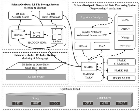
Figure 1.
Architecture of ScienceEarth prototype.
The body of ScienceEarth consists of three main parts, that is, ScienceGeoData, ScienceGeoIndex, and ScienceGeoSpark. ScienceGeoData is a remote sensing data storage framework. ScienceGeoData is in charge of storing and sharing remote sensing data where the Hadoop Distributed File System HDFS [34] is placed as the basic file system. NoSQL database, namely HBase [35], is applied to store heterogeneous tiled remote sensing data. ScienceGeoIndex is a remote sensing index framework following the basic rules of quad-tree [36] and Hilbert curve [37]. The framework rules the structure of unique key for HBase and provides access for efficient and flexible query. ScienceGeoSpark is an easy-to-use computing framework on top of the Hadoop YARN [38]. The core computation engine of ScienceGeoSpark is Spark [39] which supports distributed in-memory computation.
2.2. ScienceGeoData: A Remote Sensing Data Storage Framework
For intensive data subscription and distribution service, it is essential to guarantee high availability of remote sensing data. ScienceGeoData take charge of storage and I/O of remote sensing data of ScienceEarth. We expect the system to maintain a large amount of ready-to-use data to provide data services for various algorithms of clients. Following this pattern, data is prestored in HBase or a HDFS; data is called and queried repeatedly in future usage and services. According to the architecture of a whole system, data stored in HBase are provided according to the "one-time storage, multiple-read" strategy. As is illustrated in Figure 1, the HDFS forms the base of ScienceGeoData to provide high-throughput access to remote sensing data. Apart from the HDFS, HBase stores formatted remote sensing data and metadata. On the basis of the HDFS, HBase provides high-speed real-time database query and read-write capabilities.
A HDFS is a powerful distributed file system where we can safely store enormous remote sensing data in any format in a cloud file system similar to the local file system. Furthermore, a HDFS does not limit the file size and total storage; TB level single remote sensing image can also be stored entirely in a HDFS. As shown in Figure 2, the remote sensing dataset is replicated as three copies in the storage system as default. Especially, some of the hotspot remote sensing data can replicate more copies to meet the requirements of the frequent subscriptions. Following this manner, data are secured with multi-transcript stored in different nodes which guarantees that central remote sensing data is not lost even if some of the servers are down. For remote sensing stored in a HDFS, metadata is stored in HBase. To reach the targeted remote sensing data, a query is performed on the related HBase table to obtain the file path redirecting the file stored in a HDFS. Additionally, load balance is enabled automatically to avoid network bottleneck of single node. To sum up, a HDFS provides safe and massive cloud-based storage for remote sensing files.
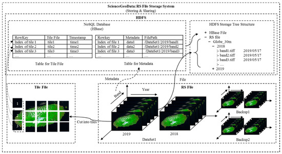
Figure 2.
Remote sensing data system with a Hadoop Distributed File System (HDFS) and HBase.
In addition to direct storage in a HDFS, we propose to also save remote sensing raster data in HBase. HBase is a columnar NoSQL database. Built upon the HDFS, HBase offers the same ability as the HDFS and guarantees security and load balance, as previously mentioned. HBase supports the storage of large quantities of data, as well as efficient query with row key. Remote sensing data stored in HBase is stored as files in the form of PNG, and each image has a fixed size. Each image in PNG format is able to store three bands of data. Such images are called tiles which is similar to the data stored in map service. The difference is that we store this data in a NoSQL database, which improves the indexing and I/O capabilities. First, giant remote sensing files are preprocessed and divided into small tile files with the same pixel size, for example, 256 pixels × 256 pixels. Each tile is, then, marked with a unique indexing row key which we can use to find the tile in a large table. In this way, users can accurately locate the spatiotemporal data required through the ScienceGeoIndex module. The large amount of remote sensing data in the data warehouse becomes "live" data. In the process of data storage, data standards and projections have also been unified. There is an interactive connection between datasets and the storage metadata has also been standardized. Under certain circumstances, for example, change detection, the task is relatively difficult if we would like to retrieve data from series of time series remote sensing data. Large amounts of related data should be queried, and certain data should be cut and mosaicked. On the contrary, serval tiles in a targeted range in different time slices are needed if we retrieve from ScienceGeoData. In such case, the efficiency has been greatly improved thanks to ScienceGeoData and ScienceGeoIndex.
2.3. ScienceGeoIndex: Remote Sensing Tile Data Index and Query Framework
It is very important to efficiently index and query remote sensing tile data. As illustrated in Figure 2, index metadata of remote sensing data stored in the HDFS is stored in HBase and remote sensing tiles in HBase are queried according to certain indexing rules. Compared with data stored in the HDFS, tiles in HBase have greater query requirements. The efficiency of index and query directly affects the overall efficiency of ScienceEarth. However, HBase’s query and indexing capabilities are not inherently powerful as only key-based queries are supported. Therefore, HBase storage indexes and queries for remote sensing data need to be optimized. In this section, we discuss the index and query of remote sensing tile data with quad-tree and Hilbert curve.
HBase supports immense unstructured data storage, as well as rapid row key index, where the efficiency of the index relies on the design of the row key. First, the row key should be as short as possible while the row key is uniquely pointed to each tile. For HBase, data are listed and indexed with the ASCII order of the row key, while continuous query is very efficient in regard to single query. Hence, we should guarantee the continuity of the row keys of which the data are spatial and time related. As illustrated in Figure 3, an example of a row key structure designed for tile data is composed of four main parts which take approximately nine chars. The first two chars represent the dataset the file belongings to. The band and year information take approximately one and two chars, respectively. The last part of the row key indicates the space location of the tile in the image.
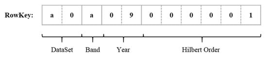
Figure 3.
Remote sensing data system with the HDFS and HBase.
Supposing that the remote sensing data are in the shape of rectangle, we divide the image into four rectangle parts with the same size. Like a quad-tree, each subpart is divided into another four parts. The upper part contains all of the four lower parts. Figure 4 shows a quad-tree with three hierarchies. At the first hierarchy, the original image is divided into four subparts, another four parts are created by each part at the next hierarchies, and the third hierarchy contains 43 tiles. Following this pattern, we divided a 30 m Landsat TM/ETM dataset covering the territory of China into nine hierarchies. The last hierarchy consisted of 49 tiles with the size of 256 × 256 pixels.
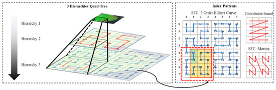
Figure 4.
Remote sensing tiles segmentation and linearization.
Each cell in the last hierarchy is marked with a unique order. There are three main methods to index each cell, hierarchy-based, space-filling curve (SFC) based, and coordinate-based indexing [21]. Hierarchy-based indexing is mostly applied for map services which provides a powerful hierarchy traversal of the cells. Compared with coordinate-based indexing, space-filling curve retains the spatial concentration of orders to the greatest extent. As illustrated in Figure 4, we propose applying the Hilbert curve to index each tile. Compared with other linearization curves, for example, Morton, Hilbert is more stable. There are more mutations in the Morton curve. For a range query in the shape of a rectangle, Hilbert orders contained in the query range are segmented continuous. For the example shown in Figure 4, the target range surrounded by red solid lines contains 12 tiles which are divided into two continuous ranges. In this example, two queries should be performed to cover the target region. For coordinate-based indexing, at least four continuous ranges should be queried. In addition, if we expand the query range from 3 × 4 to 4 × 4 which is surrounded by red dotted line, tiles can be covered by a single range. On the other hand, serval out of range tiles are queried which may cause waste of I/O resources. Balance should be considered between the efficiency of query and the waste of useless resources. We propose to optimize the query range at the last hierarchy which means all the edges of the range are extended to evens.
ScienceGeoIndex manages metadata information of remote sensing data in a HDFS. We can filter the dataset we need based on this metadata. On the basis of the quad-tree and Hilbert curve, ScienceGeoIndex defines the rules of tile indexing and ROWKEYs of each tile in database. With the indexing of remote sensing data, specialized queries could be performed easily and efficiently. Thanks to ScienceGeoIndex, ScienceGeoSpark can access remote sensing data stored in ScienceGeoData.
2.4. ScienceGeoSpark: Remote Sensing Data Processing with Spark
In this subsection, we introduce the structure of ScienceGeoSpark. As illustrated in Figure 1, data processing tasks submitted by users are uniformly scheduled by YARN. YARN is a comprehensive scheduling management system that uniformly schedules and processes job resources such as Spark and MapReduce, which provides a powerful interface for future expansion. At present, we propose Spark to deal with large-scale remote sensing data processing data. Spark is an in-memory parallel computation engine that is widely applied in different domains. As illustrated in Figure 5, according to programming paradigm of Spark, the algorithm is implemented in some programming languages, such as Java, Python, and Scala. Each programming language has a rich library of remote sensing data processing, while Spark has a rich set of components for processing machine learning [40] and databases [41]. We combine the extended library of programming languages with Spark’s operators to solve various remote sensing processing problems. Python is recommended in ScienceGeoSpark. Python is a popular programming language for image processing and machine learning thanks to its abundant libraries such as GDAL, OpenCV, Tensorflow, Keras, PyTorch, etc.
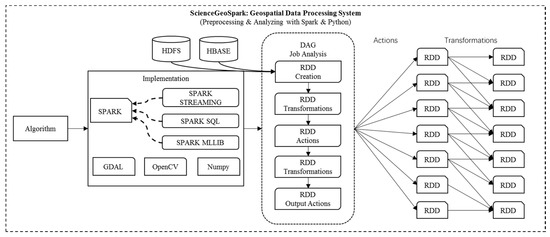
Figure 5.
Programming model with Spark and Python.
The core concept of Spark is resilient distributed datasets (RDD). All Spark operators are operations on RDD. Spark divides operators into two categories based on the principles of inertia, transformation and action. The transformation operator only records the steps of the calculation. Transformation is not executed and does not cache the results. For data-intensive computations, such as remote sensing processing, the architecture effectively saves memory resources and achieves fault tolerance and only the action operator is saved in memory. For the creation of general RDD, we need to import remote sensing data. According to the method previously mentioned, data is directly obtained from ScienceGeoData. Spark then analyzes the logic of the code, generating execution steps for calculations and processing, which are represented in the form of a directed acyclic graph. The job is then divided into a number of tasks and assigned to cluster for execution.
The advantage of this processing method is that it is suitable for the storage method of ScienceGeoData, especially for tile data stored in HBase. The data storage method in units of tiles allows calculations to be performed with any granular size. Spark’s "lazy principle" solves the contradiction between a large amount of remote sensing data and insufficient memory, and also ensures the calculation speed. Spark’s error tolerance mechanism also guarantees the stable performance of large remote sensing calculations.
2.5. Dataflow between ScienceGeoData and ScienceGeoSpark
As we all known, the first step in processing remote sensing data is to find the data we really need from the vast amount of data and, then, take targeted data out of the database to CPU or GPU for calculation. In this case, it’s the most essential issue to efficiently retrieve data instead of recording data. In this section, we focus on the dataflow of ScienceEarth.
Our main concern is to improve the comprehensive I/O efficiency of accessing these big data storage containers through ScienceEarth. As previously mentioned, there are two types of storage in ScienceGeoData. For remote sensing data stored directly in a HDFS, Spark is able to fetch data from the HDFS directly. There have been many experiments and data on testing the I/O efficiency of Hadoop and HBase [42,43,44,45,46], the I/O of both a HDFS and HBase can possibly reach serval gigabyte per second depending on the size of the files and the cluster itself. However, Python or Spark do not originally support fetching data from HBase. Therefore, we forward data with the help of Thrift. Remote sensing data are transferred trough HBase, Thrift, Python and Spark. The process is complex, and it is hard to define the overall speed by any individual step. As is illustrated in Figure 6, first, each job of Spark is analyzed and divided into a list of tasks in the task pool by the master node. The dataset required by the job is named U and consists of serval subsets corresponding to each task. Then, each idle thread of worker node in Spark cluster is assigned a task and starts to process the Python code within the task. Within each task, Python tries to demand data from HBase through Thrift. For example, Executor C processes Task 7 with tiles in (e, f). This part of data is forwarded by the Thrift node from the HBase node to Executor C. In order to reduce the workload of a single Thrift node, multiple Thrift nodes are randomly allocated to each task. Both Thrift and HBase components are distributed. In this way, the I/O load is shared by multiple executives and the entire cluster, effectively avoiding the I/O bottleneck of a single node that limits the performance of the entire platform.
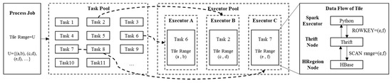
Figure 6.
Data flow between HBase and Spark.
2.6. Operation Mode of ScienceEarth
In the previous section, we explained the main components and principles of ScienceEarth and, in this section, we describe ScienceEarth from the user’s perspective. ScienceEarth is an easy-to-use big data remote sensing platform that aims to enable remote sensing scientists to conveniently experiment with large remote sensing data. ScienceEarth provides three service modules oriented for users that are based on three main components, as is shown in Figure 7. ScienceEarth provides users with data service, map service, and experiment support service.
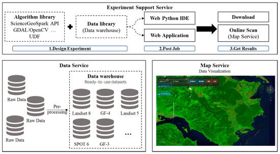
Figure 7.
Service modules of ScienceEarth, i.e., experiment support service, data service, and map service.
The data service module relies on ScienceGeoData and ScienceGeoIndex to store and manage data. Raw remote sensing data needs to be preprocessed into a data warehouse. The data in warehouse are organized with the same structure which means we can standardize the management and use of this data. We gradually upload various data to the platform’s database, hoping to provide a powerful data warehouse. Users can access remote sensing data in the data warehouse online through map service, similar to many other map services. Features such as downloading and online browsing are supported. Experiment support service is the core service of ScienceEarth. Our purpose is to provide a data-driven and algorithm-driven research service, and therefore remote sensing scientists do not need to provide their own data and most of remote sensing common algorithms. In a word, ScienceEarth provides a list of easy-to-use services.
Generally speaking, when remote sensing scientists perform experiments with ScienceEarth, first, related algorithms and data should be provided or selected from library. Subsequently, users post their task through Python or through web application online. We provide an online integrated development environment (IDE) tool, Jupyter, to process the job with Python codes. We have redeveloped many features with a simple Python application programming interface (API). The Python code should contain the basic information about some tasks, i.e., the tag name and timestamp of the dataset that are used by the ScienceGeoIndex to pinpoint the metadata stored in ScienceGeoData. Users should also specify the ScienceGeoSpark built-in algorithms or provide their own algorithm code for calculations. ScienceGeoSpark provides a standard interface for user who define their own functions. Nevertheless, serval common algorithms are developed as web-based applications. It is much easier to use application than code. Equally, the functions of web-based application are more basic. Ultimately, results are returned in different forms, such as map service or files.
3. Results
In this part of the study, we implanted an experimental ScienceEarth platform. The platform consisted of 12 virtual machines. To verify the performance of ScienceEarth, some experiments were conducted. First, we tested the I/O speed of HBase with three operations, PUT, SCAN, and ROW. Secondly, we estimated the ability of spatial concentration of the Hilbert curve. In addition, we applied ScienceEarth to perform a parallel remote sensing algorithm and compare the efficiency of ScienceEarth with a single machine.
3.1. Experiment Environment
The prototype of ScienceEarth consists of 12 nodes, of which two of the 12 are MASTER nodes which control and guarantee the runtime of ScienceEarth. The nodes are virtual machines supported by cloud. The CLIENT node is applied to submit all kinds of request by clients, communicating the clients and the platform. CLIENT node is in charge of processing all the requests from clients, we expect that the more memory should be needed for both CLIENT and MASTER nodes. For WORKER nodes, memory should pair with cores. Data is stored in each WORKER node, therefore, the storage of WORKER should be great. As illustrated in Table 1, WOEKER nodes possess 32 cores of Intel Core Processor (Skylake 2.1 GHz), 64 G of memory, and 10 TB of storage space, whereas the MASTER and CLIENT nodes possess 32 cores of Intel Core Processor (Skylake 2.1 GHz), 128 G of memory, and 5 TB of storage space. In the test, we used a set of 30 m global remote sensing data from Landsat TM/ETM dataset. This data was provided by the Institute of Remote sensing and Digital Earth.

Table 1.
Configuration and parameters of virtual machines of prototype.
3.2. Efficiency of I/O
We first tested the ability of ScienceGeoData to read and write remote sensing tile data, which is our main concern. ScienceGeoData stores and fetches remote sensing data through HBase and ScienceGeoSpark. As previously mentioned, we are mainly concerned with the remote sensing data stored in the form of tiles in HBase. These tiles are all PNG picture files. In order to simulate this kind of working situation, we randomly generated a binary file the size of which is 60 KB, simulating a picture of size 60 KB. Specifically, there are three main operations, namely PUT, ROW, and SCAN. The PUT and ROW operations separately write and read one piece of data during a single operation, whereas SCAN continuously fetches a list of data within the specified ROWKEY range from database. It should be noted that we are not encouraged to cover all targeted tiles within one SCAN operation. The working mechanism of Spark requires that large jobs be divided into small individual tasks [39]. Therefore, in order to make the work multithreaded, tiles should be covered by serval individual SCAN operations which means that we should better limit the maximum number of tiles in each single SCAN operation. Additionally, it should be noted that in the actual application situation, due to the discontinuity of the ROWKEY of the tiles, the number of tiles that each SCAN can contain varies with the situation. In this experiment, each SCAN contains 1000 tiles if not specified.
It should be considered that efficiency can be effected by the workload situation in cloud. The results can have some impact which is not caused by our algorithms or models.
3.2.1. Efficiency of I/O with Different Numbers of Working Nodes and Workload
First of all, we would like to observe the general I/O performance. The I/O workload is jointly performed by all nodes in cluster. Therefore, the number of tasks and the amount of data of the nodes participating in the work can have a certain impact on efficiency. To investigate this possible influence, we estimated the I/O efficiency under different nodes and different workloads. We tested the efficiency of three operations with different workloads, 105 tiles (5.7 GB), 5 × 10⁵ tiles (28.6 GB), 106 tiles (57.2 GB), 2 × 10⁶ tiles (114.4 GB), and 5 × 10⁶ tiles (286.1 GB). At the same time, same estimations are performed with different nodes.
As is illustrated in Figure 8, the cyan wireframe represents the results of the PUT operation, and the blue and red wireframes represent the results of the ROW and SCAN operations, separately. The axis indicates the average time cost per tile. Figure 8a, on the right, shows the detail of one slice when the tile amount is 106 tiles (57.2 GB). Under this workload, time cost declines inconspicuously with the incensement of working nodes. As shown in Figure 8b, the time cost is greater and unstable when the task load is scarce. When the tile amount is greater than 105, the efficiency stabilizes. Generally, the time cost by SCAN is the smallest, following by ROW. The PUT operation has the greatest time cost. The SCAN operation requires 0.094 ms in the most ideal situation and varies around 0.1 ms/opt. The PUT operation takes approximately 0.22 ms to operate a single tile which is approximately 2.2 times that of SCAN. The operation of PUT has the greatest time cost which varies between 0.76 ms/opt to 1.21 ms/opt. Additionally, the effect of the number of nodes and workload on efficiency is not obvious.
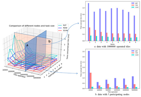
Figure 8.
Time cost per tile under different nodes and workloads for PUT, ROW, and SCAN. (a) results with 106 operated tiles; (b) results with 5 participating nodes
3.2.2. Comparison of the Efficiency of Different Data Size
We store the raster remote sensing data in a NoSQL database. However, remote sensing raster data is different from general data, its size is much larger than general vector data. The size of a single piece of data can have a similar impact on I/O efficiency. In this section, eight sets of data, ranging in size from 100 B to 60 KB, are generated randomly as the row object. Experiments of three operations are performed based on these datasets. Each test consists of 106 pieces of data and is executed on nine machines on the Spark cluster.
As shown in Figure 9, the line chart shows the speed of I/O in MB/s. This data is obtained through calculations, as well which is not real-time speed. The histogram represents the average time required to process each tile in milliseconds. The horizontal axis represents different tile sizes. We have selected a series of representative sizes from 100 B to 100 KB. The left vertical axis represents the average time required to operate each tile, and the right vertical axis represents the I/O speed. The blue line and histogram indicate PUT data, orange lines present ROW data, and green lines show SCAN operation related data. In this set of tests, SCAN operation fetches 1000 tiles per operation.
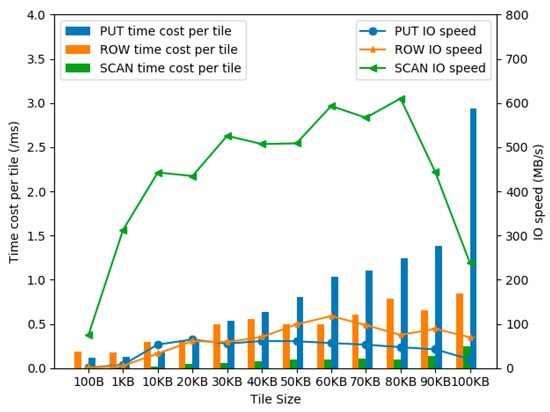
Figure 9.
Time cost per tile and I/O speed with tiles of different sizes for PUT, ROW, and SCAN.
From the histogram, it can be found that as the size of a single tile increases, the execution time required for operation also increases. It should be noted that there exist some data which are the opposite of this rule. For example, the time cost of ROW with the tile of 90 KB is greater than the time cost with the tile of 80 KB. We consider the results could have been influenced by the cloud workloads. Conversely, the I/O speed is more complex. Although the time cost of small tile is relatively low, the I/O speed is definitely not high. As is show in the line chart, at first, the speed climbs with the increasement of tile size. At some point, the I/O speed begins to decrease. Specifically, the speed of SCAN starts to fall with the size of 90 KB. The speed of ROW with the size of 60 KB is the highest and this point appears at the size of 20 KB for ROW. Additionally, when the size of tiles is smaller than 10 KB, the efficiency increases dramatically along with the size, especially for SCAN. Between 10 KB to 80 KB, the I/O speed is relatively stable.
3.2.3. Comparison of the Efficiency of SCAN
SCAN is used to obtain a series of continuous tile data in a range. By specifying a starting ROWKEY and an ending ROWKEY, SCAN sequentially obtains all the data in the interval sorted by ASCII code. It is impossible for SCAN to cover all tile data in the target at one time. First of all, the ASCII order of the ROWKEY of the tiles in the target cannot always be continuous. Secondly, the single SCAN conflicts with Spark work modes, as mentioned in Section 2.5. Meanwhile, the amount of data of each SCAN can also have a certain impact on I/O efficiency. We estimated how SCAN can affect I/O efficiency through this set of tests. Figure 10 shows the results of tests. We varied the amount of each SCAN from five tiles up to 40,000 tiles. The tested dataset consisted of 106 tiles with a size of 60 KB. Because the interval span was relatively large, we selected some characteristic points for the experiments. The abscissa represents the data amount of the tile for each SCAN query. We performed a logarithmic operation on these values in order to analyze the feature points in different intervals more intuitively and clearly. The ordinate indicates the speed of I/O in MB/s. Similarly, speed is the calculated as an average instead of real-time I/O speed.
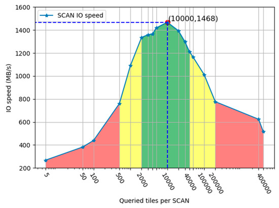
Figure 10.
I/O speed with different amounts of tiles per SCAN.
As shown in Figure 10, it is obvious that the I/O speed, firstly, grows along with the increasement of queried tiles per SCAN. When SCAN takes 10,000 tiles each time, the efficiency reaches the highest point. Subsequently, the speed starts to go down. At the top point, the I/O speed reaches 1468.3 MB/s which is 1.88 times the speed when SCAN takes 10,000 tiles each time (776.758 MB/S) and 5.49 times the speed when SCAN takes five tiles each time (267.507 MB/s). Followed by the I/O speed, the range is divided into five subranges out of three kinds. As is shown in the figure, the green range is regarded as the most efficient region while the yellow region beside the green range is acceptable. The two red regions at the both sides are of low efficiency. The results show that the I/O speed has a great relationship with the size of the SCAN.
In order to ensure the consistency of experimental conditions, previous tests were based on simulated tile data. However, for a real dataset, the size of each tile is not identical. We experimented on real datasets. The experimental dataset is a set of global 30 m three-band data, as previously mentioned. The dataset was provided by the Institute of Remote Sensing and Digital Earth, Chinese Academy of Sciences. We estimated the speed of ROW and SCAN. As illustrated in Figure 11, when the task size is larger than 105, the latency of ROW and SCAN stabilized gradually corresponding with the results of experiments in Figure 8. The average time required by ROW is approximately 0.2 ms, while SCAN takes approximately 0.1 ms, which is similar to the results of test dataset.
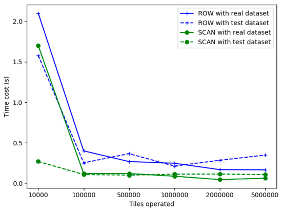
Figure 11.
Time cost per tile with 30 m Mosaic data.
3.3. Efficiency of Index and Query
The first three sets of experiments tested the I/O efficiency of the platform. However, there are many differences between the actual conditions and the experimental conditions. Experiments provide guidance for the performance improvement of the platform, but we should consider carefully the influence originated from the differences. Actually, the target area requested by the client is often restricted in a spatial polygon (we assume and simplify it into a rectangle). This range is overwritten by multiple tiles. Then, we calculate the ROWKEY of all the tiles in the range. The platform requests the corresponding data from HBase according to these ROWKEYs and performs calculations. The difference between the experiment and the actual situation is mainly reflected in two aspects. First of all, ROWKEY of the in-range data cannot be permanently contiguous, we can only represent it as multiple consecutive sets. Secondly, the size of the data is not constant. The size of a single piece of tile depends on some characteristics of each tile itself. The first question is essentially a problem associated with index methods. As mentioned in Section 3.2, continuity of ROWKEY has a significant impact on I/O efficiency. In this section, we compare the performance of the Hilbert curve with the coordinate-based method.
We estimated the ability of the spatial concentration of Hilbert curve and the coordinate-based method, which is shown in Figure 12. We simulated 5000 random rectangles that represent 5000 random query regions. The size of the queried regions varied from 100 × 100 to 1000 × 1000. The tests are performed on an 11-order quad-tree map which contains 411 × 411 tiles. The abscissa axis represents the number of tiles contained within the rectangular region, and the ordinate axis represents the number of queries required to cover all tiles in the region. Each point denotes a single simulation of region and the curves are fitted curves of the results of three different methods. Among 5000 trial queries, Hilbert (in blue) and coordinate-based (in brown) methods required a similar average number of queries. As shown in Figure 12, the fitted curves of these two methods are extremely close. It should be explained that the maximum of the coordinate-based method is defined by the number of rows or columns of the queried region. As a result, the maximum of the coordinate-based method is 1000 for the region below 1000 × 1000. Optimized Hilbert requires fewer queries to cover the same regions. When the selected area is small (0 to 4 × 10⁵ tiles), this gap is even larger.
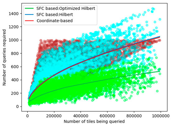
Figure 12.
Number of queries required to cover the queried region of 3 method out of a 11-order quad-tree map.
As is illustrated in Table 2, Hilbert needs 552.0326 queries while the coordinate-based method requires 546.4178 times. For optimized Hilbert, it is very obvious that after optimization, efficiency of Hilbert has been significantly improved. The number of queries required for the optimized of Hilbert is 275.4384 times on average, which is just half of the two previous methods. We extended the size of the test map to an 11-order map which contained 413 × 413 tiles. The results are illustrated in Table 2 which is almost the same as the former one. The optimized Hilbert covers the same area with fewer sets, and the size of the base map has little effect on connectivity.
Table 2.
Average number of queries of three methods with different map sizes.
3.4. Calculation Performance
In this section, we try to study the performance of ScienceGeoSpark. Previous experiments tested the I/O performance and query performance of ScienceGeoData and ScienceGeoIndex. In fact, these tasks are performed in the form of ScienceGeoSpark tasks and, although a certain amount of computing power is required in the data transmission process, the results do not reflect calculation performance. In this section, tests are based on two algorithms, high-pass filtering and edge detection, both of which are embedded originally within OpenCV.
High-pass filtering is finished through filter2D of OpenCV with a 3 × 3 kernel and edge detection is performed through operation Canny of OpenCV. For this part of the experiment, we used a set of global 30 m three-band remote sensing image data of land (without data of ocean). The row data is in the form of GeoTIFF, with a size of approximately 687 GB. In the first step, we split the data into tiles in PNG format and store the data in ScienceGeoData. It should be noted that the data in the database is approximately 296.4 GB after transformation, because the compression ratio of the PNG format is higher than that of GeoTIFF. Figure 13 shows the origin data, and data after high-pass filtering and Canny edge detection.
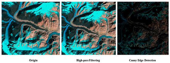
Figure 13.
Origin, high-pass filtering, and Canny edge detection.
As is shown in Figure 14, we estimated the time cost of two algorithms with different working nodes. Among these tests, the data are fetched by SCAN. As previously mentioned, SCAN data takes some of the time. In this section, we aim to eliminate this kind of influence and focus on the cost of only calculation. Therefore, we add a set of control tests with purely SCAN operations. Generally, the time cost declines when more working nodes are participating. When the working nodes increase to five, the time cost decreases slowly. With nine nodes, it takes approximately 275 s and 285 s for high-pass filtering and Canny edge detection, separately, whereas with SCAN for all the data the time cost is 205 s.
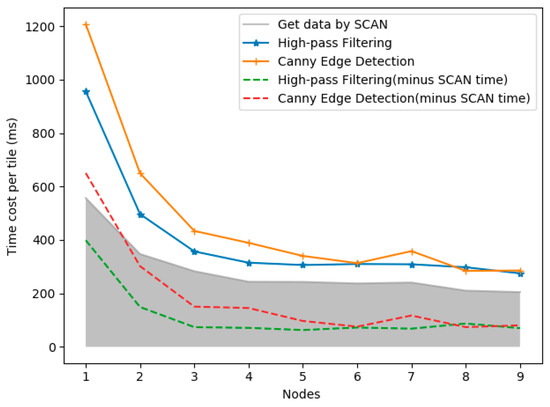
Figure 14.
Time cost of two algorithms and SCAN.
4. Discussion
4.1. Performace of the ScienceGeoData
ScienceGeoData inherits characteristics of HDFS and HBase, and ScienceGeoData is highly available and able to satisfy high I/O requests. Specifically, we store tiles data in PNG format in the database. To achieve this, we split remote sensing data into tiles with certain size of 256 × 256 pixels, following the rules of quad-trees. Following this manner, users can efficiently query and fetched data. Various complex data requirements are easily implemented in such databases. Figure 8 shows the general I/O efficiency of ScienceGeoData with tiles, there are two operations to read data from the database, SCAN and ROW, and one operation, PUT, to write into the database. Generally, speed of writing data is much lower than reading, and the performance of SCAN is more excellent than that of PUT.
In order to further explore I/O characteristics of ScienceGeoData, more experiments were carried out. Figure 9 indicates that when the tiles are in the size between 10 KB and 80 KB, the I/O speed of three main operations of HBase is stable and fine. For a PNG tile of 256 × 256 pixels with three channels, the size is exactly within the range. That is to say, the size of tile is suitable for ScienceGeoData and can reach the most efficient working condition. Figure 10 shows the I/O speed of SCAN with different SCAN sizes. We divided the range of 5 to 4 × 10⁵, into five subranges which are indicated by colors. The results suggest that SCAN size is better within 500 to 2 × 10⁵, which are shown in yellow and green.
Under experimental conditions, the I/O speed of tiles stored in HBase reach approximately 1400 MB/s when the SCAN size is 2 × 10⁴ and the single size of a tile is 60 KB. By the time this article was written, more than 80 terabytes of remote sensing data and copies had been stored in ScienceGeoData. In the whole test phase, the system of ScienceGeoData and ScienceGeoIndex has maintained stable performance.
4.2. Performance of ScienceGeoIndex
ScienceGeoIndex offers an index solution for tiles stored in SharaData. According to the quad-tree and Hilbert curve, ScienceGeoIndex retains the contiguity of ROWKEYs of the tiles. From Figure 12, the optimized Hilbert doubles the performance as compared with the coordinate-based method. When performing the same query task, optimized Hilbert only needs about half the queries as that of the coordinate-based method.
As is illustrated in Figure 15, we analyze the distribution of tiles during the simulation mentioned in Figure 12. The top bar shows the distribution of tiles in different query regions by coordinate-based index, indicating that 25% of the tiles are queried in the size of 0 to 500 tiles per SCAN, and 75% are queried in the 501 to 2000 tiles per SCAN. According to the five regions in Figure 10, the speed of 25% of the tiles is extremely low, and the speed of 75% of the tiles is relatively low. For the distribution of Hilbert in the next two bars, only 4% of tiles are in the first two regions, separately, and 37% tiles are in the third region (in green), and 42% and 12% of tiles in the two following regions. For the tiles in these two regions, we can manually split these tiles into the group of ideal size (in green). As a result, approximately 92% of tiles can be queried with high efficiency.
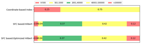
Figure 15.
Proportion of SCAN operations of different sizes with ScienceGeoIndex.
Above all, the index ability of ScienceGeoIndex is good and corresponds to the requirements of ScienceGeoData. When performing a range query, ScienceGeoIndex requires fewer queries and the structure of query is remarkable.
4.3. Performance of ScienceGeoSpark
ScienceGeoSpark offers a powerful calculation performance based on Spark, which can interact with the data in ScienceGeoData. Figure 14 shows the tests of calculation performance. It only takes about 300 s to perform edge detection on a 30 m three-band global remote sensing product with ScienceGeoSpark.
As is shown in Table 3, we compared the efficiency of ScienceGeoSpark with a normal server. The configuration of a normal server is the same as the configuration of WORKER in cluster. We processed high-pass filtering and Canny edge detection on two types of platforms with the same algorithms. First, we compared the performance for a single scene. Compared with a normal server, ScienceEarth improved the performance by 235.7% and 278.3%, separately. Although the data amount is relatively small, the advantage of ScienceEarth is limited by the basic expenditure of the system. With respect to processing the global data, the improvement reaches 2726.2% and 2406.2%. It needs to be explained that in the example with a single machine, only a single core participates in the calculation, whereas ScienceEarth has 32 cores that participate in the calculation. The same algorithm was tested on a server with 32 core parallel operations but failed because the memory required for parallel computing is too large. Although the average performance per core is reduced, ScienceEarth can calculate large tasks in parallel. At the same time, we noticed that when the number of nodes used by ScienceEarth increased from four to nine, the speed remained basically stable because the test algorithm we choose is relatively simple. The algorithm overhead is relatively small as compared with the overhead required for communication and other tasks.
Table 3.
Comparison of efficiency with ScienceEarth and a normal server.
Above all, the results manifest that ScienceEarth is a potential prototype for remote sensing big data. More complex algorithms combined with significant practical research should be tried with ScienceGeoSpark in future experiments. For example, large scale vegetation indices calculation is as suitable for cloud-based cluster framework as Google Earth Engine or ScienceEarth [47].
5. Conclusions
With the explosive growth of remote sensing data, the storage and use of remote sensing data has become a hot topic. On the other side, the development of big data technology in recent years has provided solutions and open source tools for remote sensing big data applications. Driven by the advancement of demand and the development of technology, it is possible to solve the traditional remote sensing problem through big data approaches.
In this article, we introduce a cloud-based remote sensing big data platform prototype, ScienceEarth. Composed of three main parts, i.e., ScienceGeoData, ScienceGeoIndex and ScienceGeoSpark, ScienceEarth offers a throughout solution for remote sensing data. SharaEarth is capable of storing massive amounts of heterogeneous remote sensing data and provides fast indexing of data based on various characteristics. Thanks to ScienceGeoIndex, the data stored in ScienceEarth is no longer independent and unusable raw data. ScienceEarth combines the data and processing. Remote sensing data can be directly used for fast and efficient cloud computing. Since the underlying storage and indexing of this series is transparent to users, ScienceEarth has a very low threshold for use. Thanks to the support for mainstream programming languages, ScienceEarth can be quickly and easily used by remote sensing scientists. This convenient feature allows remote sensing scientists to independently use ScienceEarth for scientific research and development. Preliminary experimental results show that the performance of ScienceEarth is excellent and it is a very promising prototype of a remote sensing data processing platform.
In subsequent work, we expect to make more progress. First, we plan to optimize the ScienceGeoIndex index structure to provide standard map services. In addition, we hope that ScienceEarth can automate the processing of raw satellite data, including geometric correction and partial radiation correction functions. Finally, we plan to introduce support for vector data and combine vector data with raster data to provide services. Machine learning and deep learning frameworks based on remote sensing images are also under consideration.
Author Contributions
Conceptualization, X.D., Z.Y. and X.F.; methodology, C.X. and X.D.; formal analysis, C.X; writing—original draft preparation, C.X. and Z.Y.; writing—review and editing, X.F., X.D. and Z.Y.; project administration, X.D. and X.F. All authors have read and agreed to the published version of the manuscript.
Funding
This work is supported by the Strategic Priority Research Program of the Chinese Academy of Sciences,
Project CASEarth (XDA19080103 and XDA19080101), the National Key Research and Development Project
(2018YFC1504201D), the National Natural Science Foundation of China (41974108) and the Key Research Program of the Chinese Academy of Sciences(KFZD-SW-317).
Acknowledgments
We thank the Open Spatial Data Sharing Project, RADI (http://ids.ceode.ac.cn/EN/) for the experimental data of Landsat TM/ETM images. At the same time, we also thank Mr. Dong Yi for his support with the experiment.
Conflicts of Interest
The authors declare no conflict of interest.
References
- Benediktsson, J.A.; Chanussot, J.; Moon, W.M. Very High-resolution remote sensing: Challenges and opportunities point of view. Proc. IEEE 2012, 100, 1907–1910. [Google Scholar] [CrossRef]
- Data, F.M.; Hou, W.; Su, J.; Xu, W.; Li, X. Inversion of the Fraction of Absorbed Photosynthetically Active Radiation (FPAR) from FY-3C MERSI Data. Remote Sens. 2020, 12, 67. [Google Scholar]
- Pinzon, J.E.; Tucker, C.J. A non-stationary 1981–2012 AVHRR NDVI3g time series. Remote Sens. 2014, 6, 6929–6960. [Google Scholar] [CrossRef]
- Ansper, A.; Alikas, K. Retrieval of chlorophyll a from Sentinel-2 MSI data for the European Union water framework directive reporting purposes. Remote Sens. 2019, 11, 64. [Google Scholar] [CrossRef]
- Drahansky, M.; Paridah, M.; Moradbak, A.; Mohamed, A.; Owolabi, F.; Abdulwahab, T.; Asniza, M.; Abdul, K.S.H. A Review: Remote Sensing Sensors. IntechOpen 2016, 17, 777. [Google Scholar]
- Gamba, P.; Du, P.; Juergens, C.; Maktav, D. Foreword to the Special Issue on Human Settlements: A Global Remote Sensing Challenge. IEEE J. Sel. Top. Appl. Earth Obs. Remote Sens. 2011, 4, 5–7. [Google Scholar] [CrossRef]
- He, G.; Wang, L.; Ma, Y.; Zhang, Z.; Wang, G.; Peng, Y.; Long, T.; Zhang, X. Processing of earth observation big data: Challenges and countermeasures. Kexue Tongbao Chin. Sci. Bull. 2015, 60, 470–478. [Google Scholar]
- Bhardwaj, A.; Sam, L.; Akanksha, B.; Martín-Torres, F.J.; Kumar, R. UAVs as remote sensing platform in glaciology: Present applications and future prospects. Remote Sens. Environ. 2016, 175, 196–204. [Google Scholar] [CrossRef]
- Zhang, X.; Zhang, F.; Qi, Y.; Deng, L.; Wang, X.; Yang, S. New research methods for vegetation information extraction based on visible light remote sensing images from an unmanned aerial vehicle (UAV). Int. J. Appl. Earth Obs. Geoinf. 2019, 78, 215–226. [Google Scholar] [CrossRef]
- Klemas, V.V. Coastal and Environmental Remote Sensing from Unmanned Aerial Vehicles: An Overview. J. Coast. Res. 2015, 315, 1260–1267. [Google Scholar] [CrossRef]
- Prinz, T.; Lasar, B.; Krüger, K.P. High-resolution remote sensing and GIS techniques for geobase data supporting archaeological surveys: A case study of ancient doliche, southeast Turkey. Geoarchaeology 2010, 25, 352–374. [Google Scholar] [CrossRef]
- Guo, H.; Wang, L.; Chen, F.; Liang, D. Scientific big data and Digital Earth. Chin. Sci. Bull. 2014, 59, 5066–5073. [Google Scholar] [CrossRef]
- Wang, L.; Ma, Y.; Zomaya, A.Y.; Ranjan, R.; Chen, D. A parallel file system with application-aware data layout policies for massive remote sensing image processing in digital earth. IEEE Trans. Parallel Distrib. Syst. 2015, 26, 1497–1508. [Google Scholar] [CrossRef]
- Oliveira, S.F.; Fürlinger, K.; Kranzlmüller, D. Trends in computation, communication and storage and the consequences for data-intensive science. In Proceedings of the 2012 IEEE 14th International Conference on High Performance Computing and Communication & 2012 IEEE 9th International Conference on Embedded Software and Systems, Liverpool, UK, 25–27 June 2012; pp. 572–579. [Google Scholar]
- Zhong, Y.; Ma, A.; Ong, Y.S.; Zhu, Z.; Zhang, L. Computational intelligence in optical remote sensing image processing. Appl. Soft Comput. J. 2018, 64, 75–93. [Google Scholar] [CrossRef]
- Huang, B.; Jin, L.; Lu, Z.; Yan, M.; Wu, J.; Hung, P.C.K.; Tang, Q. RDMA-driven MongoDB: An approach of RDMA enhanced NoSQL paradigm for large-Scale data processing. Inf. Sci. 2019, 502, 376–393. [Google Scholar] [CrossRef]
- Li, C.; Yang, W. The distributed storage strategy research of remote sensing image based on Mongo DB. In Proceedings of the 2014 3rd International Workshop on Earth Observation and Remote Sensing Applications (EORSA), Changsha, China, 11–14 June 2014; pp. 101–104. [Google Scholar]
- Liu, X.; Han, J.; Zhong, Y.; Han, C.; He, X. Implementing WebGIS on Hadoop: A case study of improving small file I/O performance on HDFS. In Proceedings of the 2009 IEEE International Conference on Cluster Computing and Workshops, New Orleans, Louisiana, 31 August–4 September 2009; pp. 1–8. [Google Scholar]
- Lin, F.C.; Chung, L.K.; Ku, W.Y.; Chu, L.R.; Chou, T.Y. The framework of cloud computing platform for massive remote sensing images. In Proceedings of the 2013 IEEE 27th International Conference on Advanced Information Networking and Applications (AINA), Barcelona, Spain, 25–28 March 2013; pp. 621–628. [Google Scholar]
- Xiao, Z.; Liu, Y. Remote sensing image database based on NOSQL database. In Proceedings of the 2011 19th International Conference on Geoinformatics, Shanghai, China, 24–26 June 2011; pp. 3–7. [Google Scholar]
- Mahdavi-Amiri, A.; Alderson, T.; Samavati, F. A Survey of Digital Earth. Comput. Graph. 2015, 53, 95–117. [Google Scholar] [CrossRef]
- Fan, J.; Yan, J.; Ma, Y.; Wang, L. Big data integration in remote sensing across a distributed metadata-based spatial infrastructure. Remote Sens. 2018, 10, 7. [Google Scholar] [CrossRef]
- Wei, L.Y.; Hsu, Y.T.; Peng, W.C.; Lee, W.C. Indexing spatial data in cloud data managements. Pervasive Mob. Comput. 2014, 15, 48–61. [Google Scholar] [CrossRef]
- Lin, A.; Chang, C.F.; Lin, M.C.; Jan, L.J. High-performance computing in remote sensing image compression. High. Perform. Comput. Remote Sens. 2011, 8183, 81830C. [Google Scholar]
- Yan, J.; Ma, Y.; Wang, L.; Choo, K.K.R.; Jie, W. A cloud-based remote sensing data production system. Futur. Gener. Comput. Syst. 2018, 86, 1154–1166. [Google Scholar] [CrossRef]
- Ayguadé, E.; Copty, N.; Duran, A.; Hoeflinger, J.; Lin, Y.; Massaioli, F.; Teruel, X.; Unnikrishnan, P.; Zhang, G. The design of OpenMP tasks. IEEE Trans. Parallel Distrib. Syst. 2009, 20, 404–418. [Google Scholar] [CrossRef]
- Dean, J.; Ghemawat, S. MapReduce: Simplified data processing on large clusters. Commun. ACM 2008, 51, 107–113. [Google Scholar] [CrossRef]
- Lv, Z.; Hu, Y.; Zhong, H.; Wu, J.; Li, B.; Zhao, H. Parallel K-Means Clustering of Remote Sensing images Based on Mapreduce. Available online: https://www.researchgate.net/publication/220774985_Parallel_K-Means_Clustering_of_Remote_Sensing_Images_Based_on_MapReduce (accessed on 11 February 2020).
- Wang, L.; Ma, Y.; Yan, J.; Chang, V.; Zomaya, A.Y. pipsCloud: High performance cloud computing for remote sensing big data management and processing. Futur. Gener. Comput. Syst. 2018, 78, 353–368. [Google Scholar] [CrossRef]
- Gorelick, N.; Hancher, M.; Dixon, M.; Ilyushchenko, S.; Thau, D.; Moore, R. Google Earth Engine: Planetary-scale geospatial analysis for everyone. Remote Sens. Environ. 2017, 202, 18–27. [Google Scholar] [CrossRef]
- Bioucas-Dias, J.M.; Plaza, A.; Camps-Valls, G.; Scheunders, P.; Nasrabadi, N.M.; Chanussot, J. Hyperspectral remote sensing data analysis and future challenges. IEEE Geosci. Remote Sens. Mag. 2013, 1, 6–36. [Google Scholar] [CrossRef]
- Sefraoui, O.; Aissaoui, M.; Eleuldj, M. OpenStack: Toward an Open-source Solution for Cloud Computing. Int. J. Comput. Appl. 2012, 55, 38–42. [Google Scholar] [CrossRef]
- Grossman, R.L. The case for cloud computing. IT Prof. 2009, 11, 23–27. [Google Scholar] [CrossRef]
- Borthakur, D. HDFS Architecture Guide. Available online: https://hadoop.apache.org/docs/current/hadoop-project-dist/hadoop-hdfs/HdfsDesign.html (accessed on 11 February 2020).
- Vora, M.N. Hadoop-HBase for large-scale data. In Proceedings of the 2011 International Conference on Computer Science and Network Technology, Harbin, China, 24–26 December 2011; Volume 1, pp. 601–605. [Google Scholar]
- Zhang, J.; You, S.; Gruenwald, L. Parallel quadtree coding of large-scale raster geospatial data on GPGPUs. In Proceedings of the 19th ACM SIGSPATIAL International Conference on Advances in Geographic Information Systems, Gosier, Guadeloupe, France, 23–28 February 2011; pp. 457–460. [Google Scholar]
- Jing, W.; Tian, D. An improved distributed storage and query for remote sensing data. Procedia Comput. Sci. 2018, 129, 238–247. [Google Scholar] [CrossRef]
- Vavilapalli, V.; Murthy, A. Apache Hadoop Yarn: Yet Another Resource Negotiator Big Data Resources Scheduling. Available online: https://www.cse.ust.hk/~weiwa/teaching/Fall15-COMP6611B/reading_list/YARN.pdf (accessed on 11 February 2020).
- Zaharia, M.; Chowdhury, M.; Franklin, M.J.; Shenker, S.; Stoica, I. Spark: Cluster computing with working sets. HotCloud 2010, 10, 95. [Google Scholar]
- Meng, X.; Bradley, J.; Yavuz, B.; Sparks, E.; Venkataraman, S.; Liu, D.; Freeman, J.; Tsai, D.B.; Amde, M.; Owen, S.; et al. MLlib: Machine learning in Apache Spark. J. Mach. Learn. Res. 2016, 17, 1–7. [Google Scholar]
- Qin, V.L. Spark SQL Relational Data Processing in Spark. Acad. Psychiatry 2017, 41, 763. [Google Scholar] [CrossRef]
- Zhang, Y.; Liu, D. Improving the efficiency of storing for small files in hdfs. In Proceedings of the Computer Science & Service System (CSSS), Nanjing, China, 11–13 August 2012; pp. 2239–2242. [Google Scholar]
- Xue, S.J.; Pan, W.B.; Fang, W. A novel approach in improving I/O performance of small meteorological files on HDFS. Appl. Mech. Mater. 2012, 117, 1759–1765. [Google Scholar] [CrossRef]
- Yang, X.; Yin, Y.; Jin, H.; Sun, X.H. SCALER: Scalable parallel file write in HDFS. In Proceedings of the 2014 IEEE International Conference on Cluster Computing (CLUSTER), Madrid, Spain, 22–26 September 2014; pp. 203–211. [Google Scholar]
- Chebotko, A.; Abraham, J.; Brazier, P.; Piazza, A.; Kashlev, A.; Lu, S. Storing, indexing and querying large provenance data sets as RDF graphs in apache HBase. In Proceedings of the Services (SERVICES), 2013 IEEE Ninth World Congress on Services, Santa Clara, CA, USA, 28 June–3 July 2013; pp. 1–8. [Google Scholar]
- Azqueta-Alzuaz, A.; Patino-Martinez, M.; Brondino, I.; Jimenez-Peris, R. Massive data load on distributed database systems over HBase. In Proceedings of the 2017 17th IEEE/ACM International Symposium on Cluster, Cloud and Grid Computing (CCGRID), Madrid, Spain, 14–17 May 2017; pp. 776–779. [Google Scholar]
- Silva-Junior, C.A.D.; Leonel-Junior, A.H.S.; Rossi, F.S.; Correia-Filho, W.L.F.; Santiago D de, B.; de Oliveira-Júnior, J.F.; Teodoro, P.E.; Lima, M.; Capristo-Silva, G.F. Mapping soybean planting area in midwest Brazil with remotely sensed images and phenology-based algorithm using the Google Earth Engine platform. Comput. Electron. Agric. 2020, 169, 105194. [Google Scholar] [CrossRef]


© 2020 by the authors. Licensee MDPI, Basel, Switzerland. This article is an open access article distributed under the terms and conditions of the Creative Commons Attribution (CC BY) license (http://creativecommons.org/licenses/by/4.0/).