Article

Mapping the Land Cover of Africa at 10 m Resolution from Multi-Source Remote Sensing Data with Google Earth Engine

1
Remote Sensing Technology Institute (IMF), German Aerospace Center (DLR), 82234 Wessling, Germany
2
Signal Processing in Earth Observation, Technical University of Munich (TUM), 80333 Munich, Germany
*
Author to whom correspondence should be addressed.
Remote Sens. 2020, 12(4), 602; https://doi.org/10.3390/rs12040602
Submission received: 2 December 2019 / Revised: 5 February 2020 / Accepted: 5 February 2020 / Published: 11 February 2020
(This article belongs to the Special Issue Regional and Global Land Cover Mapping)

Abstract

:
The remote sensing based mapping of land cover at extensive scales, e.g., of whole continents, is still a challenging task because of the need for sophisticated pipelines that combine every step from data acquisition to land cover classification. Utilizing the Google Earth Engine (GEE), which provides a catalog of multi-source data and a cloud-based environment, this research generates a land cover map of the whole African continent at 10 m resolution. This land cover map could provide a large-scale base layer for a more detailed local climate zone mapping of urban areas, which lie in the focus of interest of many studies. In this regard, we provide a free download link for our land cover maps of African cities at the end of this paper. It is shown that our product has achieved an overall accuracy of 81% for five classes, which is superior to the existing 10 m land cover product FROM-GLC10 in detecting urban class in city areas and identifying the boundaries between trees and low plants in rural areas. The best data input configurations are carefully selected based on a comparison of results from different input sources, which include Sentinel-2, Landsat-8, Global Human Settlement Layer (GHSL), Night Time Light (NTL) Data, Shuttle Radar Topography Mission (SRTM), and MODIS Land Surface Temperature (LST). We provide a further investigation of the importance of individual features derived from a Random Forest (RF) classifier. In order to study the influence of sampling strategies on the land cover mapping performance, we have designed a transferability analysis experiment, which has not been adequately addressed in the current literature. In this experiment, we test whether trained models from several cities contain valuable information to classify a different city. It was found that samples of the urban class have better reusability than those of other natural land cover classes, i.e., trees, low plants, bare soil or sand, and water. After experimental evaluation of different land cover classes across different cities, we conclude that continental land cover mapping results can be considerably improved when training samples of natural land cover classes are collected and combined from areas covering each Köppen climate zone.

1. Introduction

Land cover mapping is considered to be one of the most important tasks in remote sensing, as it provides crucial geoinformation for environmental research. Since physical characteristics are closely related to the land cover type, the land cover classes not only relate to the local ecosystems but also to the climate system. This knowledge of regional land cover classes is of great relevance to land use management, including nature conservation, water management, agricultural monitoring, etc. Large-scale land cover maps of extended areas, such as whole countries or even continents, provide abundant information for policy-makers making decisions and taking action for sustainable development. Existing large-scale land cover mapping products are (1) MODIS Global Land Cover [1]; (2) ESA GlobCover [2]; (3) UMD classification [3]; (4) CCI-LC [4]; (5) GLC-SHARE [5]; (6) GLCNMO [6]; and (7) Copernicus Global Land Cover [7]. However, these land cover products are limited to coarse spatial resolution in the range of 100 m and 1 km, and this provides insufficient spatial detail. Existing high resolution global land cover products are (1) FROM-GLC10 [8]; (2) FROM-GLC30 [9]; and (3) GlobeLand30 [10], but they are only available for certain years, and not updated regularly.
Google Earth Engine (GEE) has been recognized as a substantial enabler of large-scale mapping, with its powerful capabilities in accessing and processing massive volumes of multi-source, multi-temporal, multi-scale Earth Observation (EO) data through a cloud platform [11]. Available datasets in the GEE catalog include satellite imagery, geophysical data, climate and weather data, and demographic data. In this regard, GEE provides exciting opportunities for multi-temporal and large-scale land cover mapping [12,13,14,15]. However, most existing studies focus on one specific land cover type or only generate land cover maps for certain regions at a specific image acquisition time. Therefore, these studies are often difficult to scale up to continental or global areas at other times.
Africa has the fastest population growth compared to other continents [16], and environmental threats such as erosion, desertification, deforestation, drought, and water shortages often have detrimental impacts on the continent’s development in Africa [17]. Therefore, providing regularly updated land cover maps is vital to land management in Africa, as these maps offer information related to the protection of terrestrial ecosystems and livelihoods of the continent. Currently, there are only two African land cover products derived from GEE: FROM-GLC10 and AfricaLC [18]. There are multi-source data available in GEE, which not only could reduce data gaps and uncertainties of individual data sources, but also could improve the classification results [19]. However, both FROM-GLC10 and AfricaLC have not fully harnessed the available data on GEE, and have failed to provide an analysis of influences from different combinations of the data sources. Moreover, the creation of training samples for large-scale land cover mapping takes a large quantity of time and manual work. For example, in order to ensure that training samples are representative for the whole continent, AfricaLC selects the training samples from all 49 countries in continental Africa. This manual work could be reduced if the trained models that use samples created for some cities could be implemented to classify a different city into its land cover types, a process that is referred to as transferability [20] and has not been adequately addressed in the current literature. In this research, we propose a framework for land cover mapping in Africa from multi-source data with GEE, which makes three main contributions:
(1) The proposed framework is able to provide reliable land cover maps of the whole African continent at a resolution of 10 m, using GEE’s multi-source remote sensing data.
(2) With the ready-to-use availability of multi-source data in GEE, we have investigated the data and feature importance within the multi-source data-based framework for continental scale land cover mapping, which has not been adequately addressed in the current literature. This is performed by gradually introducing different data and feature importance analysis based on the classifier used. As a result, the best input configurations are determined and applied in this study.
(3) In order to offer useful sampling strategies for similar continental land cover mapping tasks, we have investigated the transferability issue further by using reference data of selected cities across the African continent and employing the processing and data resources in GEE. It should be noted that this work is in a advanced position to study the transferability of trained models for different land cover classes in the continental scale land cover mapping.
The remainder of this paper is structured as follows: Section 2 introduces the study area and data considered in this research. In Section 3, the proposed framework for land cover mapping and the experiment setup are described. The quantitative and qualitative results are presented in Section 4. Section 5 provides a detailed discussion of the results. Finally, Section 6 summarizes and concludes the work.

2. Study Area and Dataset
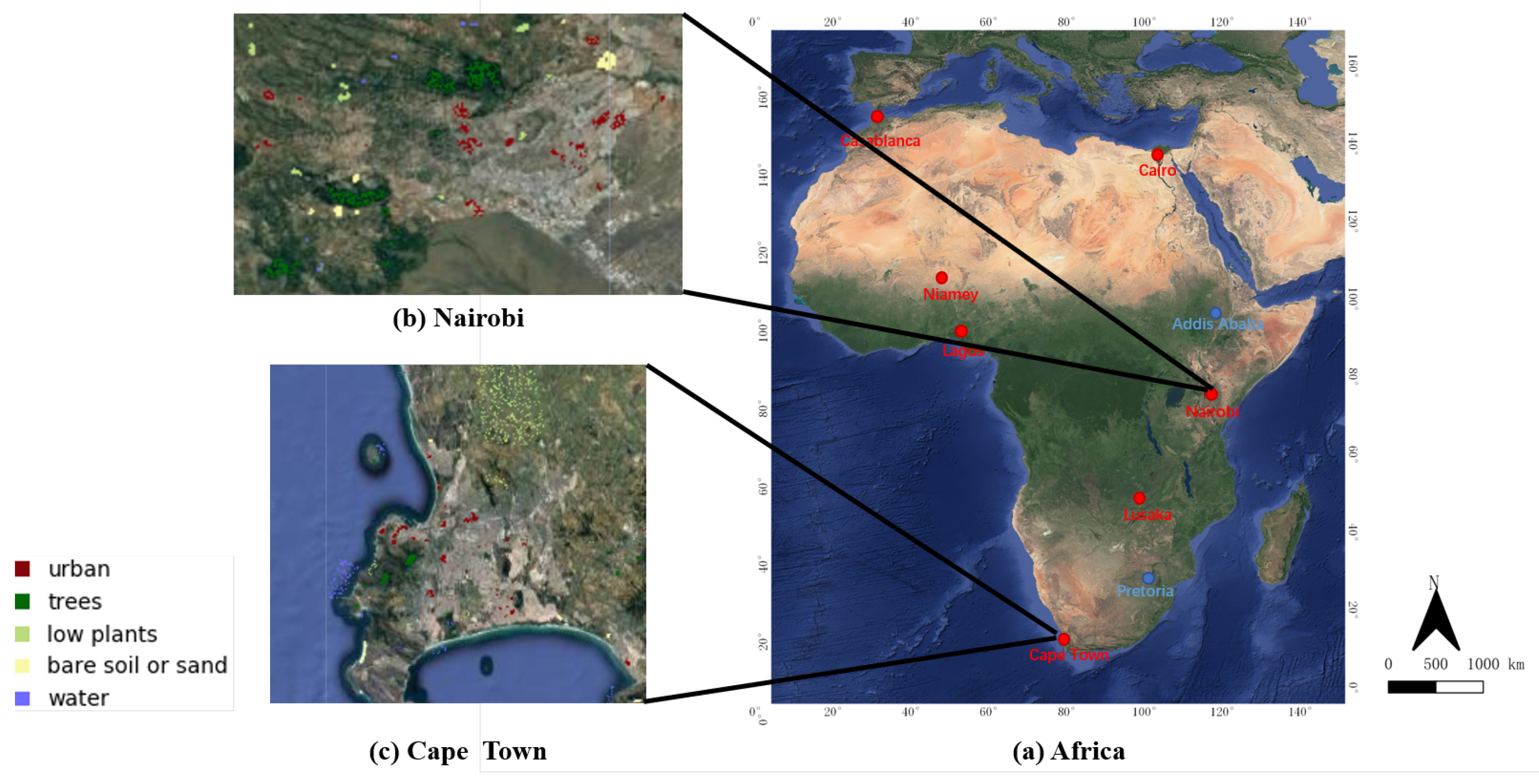
2.1. Study Area

The entire continent of Africa is selected as the study area in this research. Africa has the second largest population of all seven continents, which amounted to about 1.2 billion people in 2016. Moreover, Africa is the second largest continent (covering an area of 30.3 million km 2 ), extending from 37°N to 34°S in latitude and from 51°E and 17°W in longitude. Thus, the climate varies widely across different African regions, ranging from a tropical climate to a Mediterranean climate. Similarly, its geography is extremely diverse: the northern half of the continent is mainly desert, while the central and southern parts are primarily forest regions.

2.2. Multi-Source Geodata for Land Cover Mapping

  • Sentinel-2 Satellite Imagery
    Sentinel-2 consists of 13 spectral bands, which includes four bands with 10 m spatial resolution, six bands with 20 m spatial resolution, and three bands with 60 m spatial resolution, as shown in Table 1. In the GEE catalog, Sentinel-2 Multispectral Instrument (MSI), Level-1C data [21] is the standard of the Sentinel-2 archive, and represents the Top Of Atmosphere (TOA) reflectance. For this study, Bands 1, 9, and 10 are excluded, as they contain only information about the atmosphere rather than land surface data, and only have a coarse spatial resolution.
  • Landsat-8 Satellite Imagery
    Landsat-8 [22] consists of two science instruments: the Operational Land Imager (OLI) and the Thermal Infrared Sensor (TIRS). OLI collects data from eight spectral bands at 30 m and one panchromatic band at 15 m. TIRS conducts thermal imaging from two bands at 100 m, as shown in Table 1. In this research, Landsat-8 Surface Reflectance Tier 1 is chosen as the input data. This data is orthorectified and atmospherically corrected surface reflectance, which excludes Band 8 and 9.
  • Night Time Light (NTL) Data
    The Visible Infrared Imaging Radiometer Suite (VIIRS) Day/Night Band (DNB) [23], sourced from the Suomi National Polar-orbiting Partnership (Suomi-NPP) satellite, is able to provide multi-temporal NTL data, which allows near-real-time monitoring because of its high repeat frequency. For this study, we use VIIRS DNB Composites Version 1 data, which is the temporal average radiance on a monthly basis at 742 m spatial resolution.
  • Global Human Settlement Layer (GHSL)
    Human settlement information is derived for the four different epochs 1975, 1990, 2000, and 2014 in GHSL [24]. From the GHSL data (Built-Up Grid 1975-1990-2000-2015 (P2016)) available in the GEE catalog, the “built” class identifies the presence of built-up areas at 38 m spatial resolution.
  • Shuttle Radar Topography Mission (SRTM)
    The SRTM V3 product (SRTM Plus) [25] is exploited in our research, which is an enhanced version of the original digital elevation model (DEM) at 30 m spatial resolution. The slope in degrees from the DEM is adopted in this research, which is the local gradient within the four-connected neighbors of each pixel.
  • MODIS Land Surface Temperature (LST)
    MODIS is an imaging sensor on both the Terra and Aqua satellites, which aim to acquire global dynamics of the Earth. LST can be derived from the radiance at Band 31 and 32 that is measured with the Terra satellite. In this study, we chose MYD11A2 V6 [26] available in GEE as MODIS LST. MYD11A2 V6 is a simple average of the data collected within that eight-day period, which can provide both day and night LST with a 1 km spatial resolution.

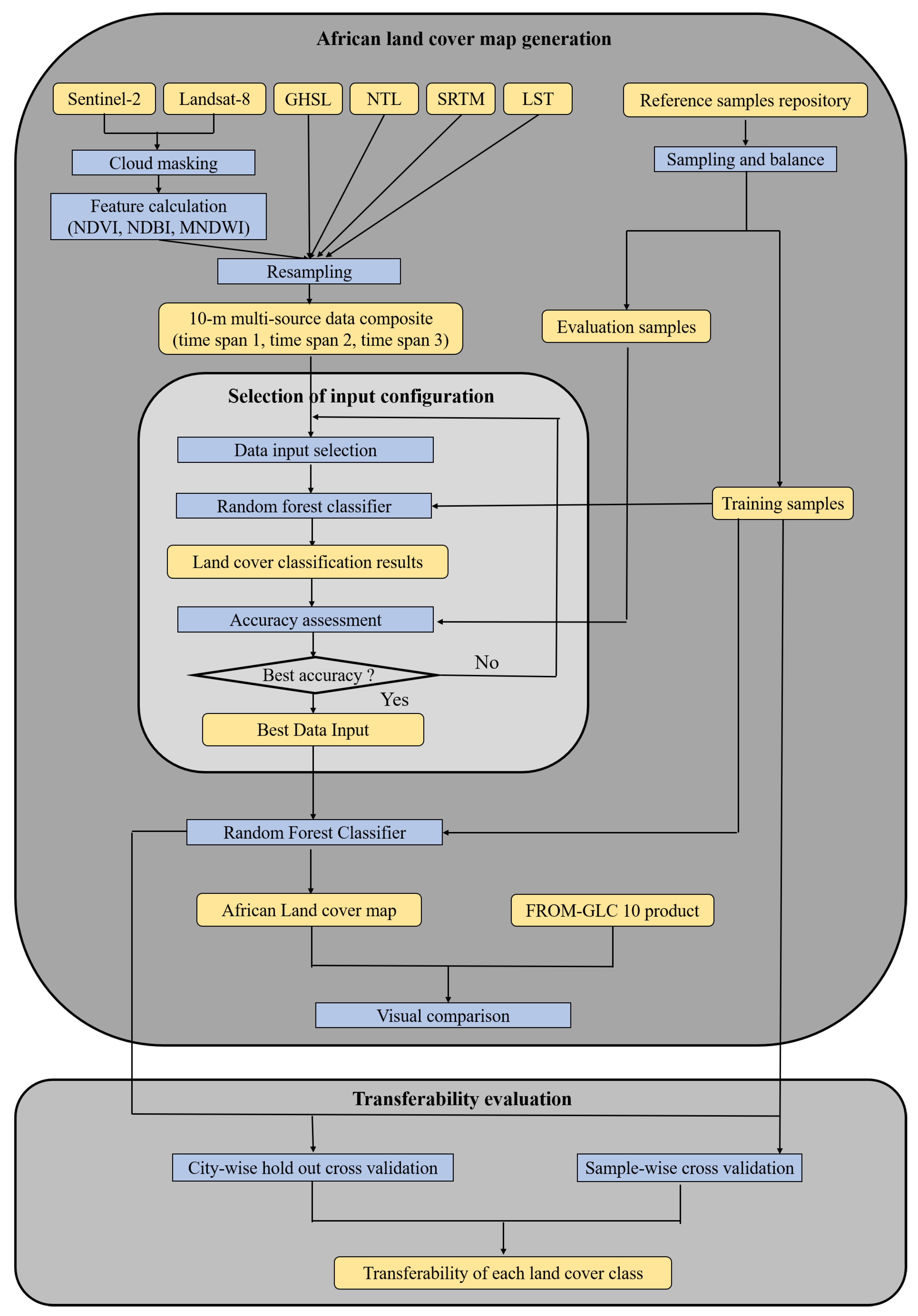
3. A Framework for Land Cover Mapping from Multi-Source Data

3.1. Overview of the Proposed Framework

Figure 1 shows a comprehensive overview of the proposed framework, which can be utilized as a routine strategy for large-scale land cover mapping. The proposed framework presented in this research makes three key contributions to the extant literature: (1) African land cover map generation (2) selection of input configurations, and (3) transferability evaluation, where each part is closely linked to the other parts. After the data preprocessing steps, such as cloud masking from Sentinel-2 and Landsat-8 data, the features of these two input sources are extracted in the form of selected spectral indices. Then each employed data is processed as follows. Firstly, we collected all the available data within each of the three time spans, (January–April 2017; May–August 2017; September–December 2017). Then, the composite for each time span is then produced by taking the median pixel value from all the collected data. Finally, a composite of multi-source data at a spatial resolution of 10 m, where all different datasets are stacked together, is built for all three time spans. This is based on the assumption that the land cover classes will remain stable for a year. The best data input is yielded after the selection of input configurations. In this research, a Random Forest (RF) classifier is used to classify the mosaics for each temporal composition into different land cover classes. Finally, the land cover map is produced after the majority voting of the results from the three time spans, a process that compensates for the data missing from certain time spans. In the sampling step, all the reference samples are manually selected around the nine selected African cities, and are divided into training and evaluation samples. We then investigate the transferability of trained models derived from training samples for different land cover classes, based on the experiments of transferability evaluation, which include “city-wise holdout cross validation” and “sample-wise cross validation”.

3.2. African Land Cover Map Generation

3.2.1. Preprocessing
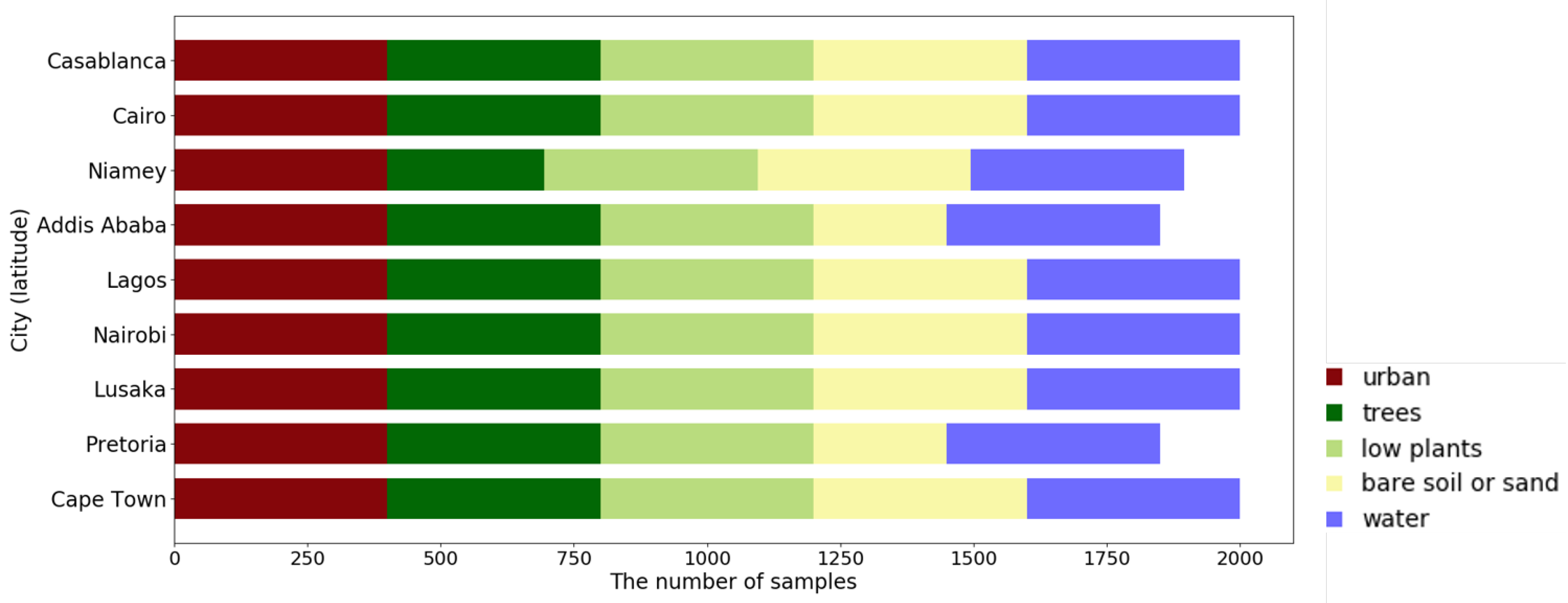
For optical satellite imagery, cloud cover is an important factor that affects the potential of this form of imagery for land cover mapping. The “pixel_ qa” band of Landsat-8 is a bitmask band, which contains a quality attribute generated from the CFMASK algorithm [27] and can be utilized to remove cloud. For Sentinel-2 imagery, the simple cloud detection algorithm proposed in [28] is implemented to mask clouds.
Spectral indices are widely used in the existing literature on large-scale land cover mapping [3]. They are based on expert knowledge of the known characteristics of land cover classes, such as urban, vegetation, and water. Thus, we adopt three popular spectral indices: the normalized difference built-up index (NDBI) [29], the normalized difference vegetation index (NDVI) [30], and the modified normalized difference water index (MNDWI) [31], which are a recommended feature combination for land cover classification in [32]. These three spectral indices are closely related to the land cover classes defined in our research; and their formulas are summarized in Table 2.
After the features are calculated from both Sentinel-2 and Landsat-8 satellite imagery using the above spectral indices, all the multi-source data are resampled to 10 m spatial resolution, which corresponds to the fine resolution of Sentinel-2. Finally, all the data are projected into the GCS WGS84 coordinate system. All these steps can be undertaken internally and seamlessly on the GEE platform.

3.2.2. Sampling

Inspired by the local climate zone classification scheme [33,34,35], which is related to the physical nature of surface properties, in this research we select five land cover classes—(1) urban, (2) trees, (3) low plants, (4) bare soil or sand, and (5) water. Urban consists of different building types and impervious ground such as paved surfaces. Trees represent wooded landscapes such as trees or bushes on pervious ground. Low plants include natural grassland, agriculture, and urban recreation. Bare soil or sand describes a featureless landscape of pervious ground. Water includes open water bodies such as rivers, oceans, and lakes.
In order to select the most representative land cover samples to map the whole African continent, seven cities—Cairo, Cape Town, Nairobi, Lagos, Niamey, Lusaka, and Casablanca—are chosen as training cities. The samples in these cities provide a complete representation of different land cover classes. These seven cities are located in widely different geographic environments. Specifically, according to the Köppen climate classification system [36], the training cities belong to eight different climate zones, which represent the eight climate types in Africa. The socioeconomic characteristics (e.g., population and economy) of these training cities also vary considerably. In order to select the best input configurations and evaluate the generated African land cover map, we select two cities—Addis Ababa and Pretoria—as evaluation cities. The geographic distribution and climate type of training and evaluation cities is illustrated in Figure 2a and Table 3, respectively.
We obtained all reference land cover samples in the nine selected cities by manual interpretation from very high spatial resolution satellite imagery. In order to ensure a good representation of different land cover classes, all reference samples are distributed in not only city areas but also rural areas. Each sample is extracted within a 10 × 10 m area from every Region of Interest (ROI), which also ensures the homogeneity and geographic integrity of the samples. Then we make a selection of random samples for each land cover class within each city. The distribution of each land cover class among different cities is illustrated in Figure 3. The distribution of the reference samples collected from the study area in Nairobi and Cape Town are illustrated in Figure 2b,c, and we randomly select 400 sample points for each land cover class in these two cities.

3.2.3. Random Forest Classifier

There are many automatic classification algorithms for land cover classification in GEE, such as maximum likelihood classification (MLC), RF, and support vector machine (SVM) [36]. In this research, an RF [37] classifier is chosen as the supervised classification method for land cover mapping, which has advantages in flexibility and speed when dealing with large datasets [38]. RF can not only manage multi-dimension data [39] such as multi-source data [40], but can also realize multi-feature fusion, where feature selection is closely linked with learning phases [41]. RF is an ensemble-based classifier that consists of many classification decision trees. Each decision tree gives a class label to the pixel by classification, and the pixel is finally assigned the class label with the most votes. For each of the decision trees, only a subsection of the training data is used; thus, the overfitting issue can be controlled. Here, we use 50 trees, as suggested in [9], which can simultaneously meet the accuracy and computation speed requirements for large-scale land cover classification problems.
Another function of RF, where the importance of each feature can be derived, has elicited an increasing interest in the RS domain [42]. The mean decrease in Gini (MDG) [37] is defined as the amount of decrease in the node impurity criterion resulting from each feature, which is an indicator to estimate the feature importance [41]. It should be noted that the RF method is preferred in this study not only because it is able to assign a land cover class label to each pixel, but also because it can be used to derive the importance of the multiple input features [43,44].

3.2.4. Accuracy Assessment

The most widely used statistical accuracy assessment method in land cover classification is the confusion matrix [45], which is a cross-tabulation of the predicted class label against that in the ground reference. Some accuracy measures can be derived from the confusion matrix, such as overall accuracy, kappa, and the user’s accuracy and producer’s accuracy for each class. Overall accuracy (OA) is the percentage of pixels assigned with the correct label. Kappa is also a measure to assess the overall agreement between classification and ground reference. If we want to focus on the accuracy of an individual class, then the user’s and producer’s accuracy are the most important measures. The user’s accuracy indicates the percentages of pixels that are incorrectly classified as a known class. The producer’s accuracy represents the percentage of pixels of a known class that are classified as other classes. The F1-score indicates a balance between the user’s accuracy and the producer’s accuracy. For a qualitative accuracy assessment, FROM-GLC10 product, which is an existing global land cover map at 10 m, has been selected as a visual comparison of our African land cover map.

3.3. Selection of Input Configurations

Since multi-source data are used in our research, we are concerned about which input configurations will eventually provide the best accuracy of land cover classification. In this regard, one of the contributions of our research is the investigation of multi-source data in land cover classification.
Different data aid in the discrimination of land cover classes based on their different features. Sentinel-2 and Landsat-8 satellite imagery offer global high and medium resolution multi-spectral data of the Earth’s surface, respectively, which characterize different land cover classes based on spectral information [14]. GHSL presents the global spatial representation of human settlement during the past 40 years, which is closely linked with the urban class [46]. NTL data monitors the nighttime world with one of signal sources from city lights, so that it can also be utilized to map urban areas or human settlements [47]. The high-quality global SRTM DEM is anticipated to regulate differences in land cover distribution [48]. In addition, many studies have tested the sensitivity of climate such as LST to land cover compositions [49].
In order to select the best input data, we designed an experiment called “fixed validation”. In this experiment, the reference samples for all seven training cities were utilized to train the model, and accuracy measures were derived for the two evaluation cities. This experiment has two applications: one to generate a land cover map of the whole African continent by finding the best input configurations, and the other for comparison with other experiments, where only reference samples of a subset of training cities are exploited for the model training.
Based on the experiment of “fixed validation”, we first use only Sentinel-2 data to obtain land cover classification results. Then, the features extracted from Sentinel-2 and other multi-source data are gradually introduced as input configurations. The new introduced data will only be accepted when there is an improvement in the accuracy indexes. Finally, the best input configurations can be selected based on the best achievable accuracy.

3.4. Transferability Evaluation

Another contribution of our research is to explore transferability issues using training data for selected cities around Africa. To this end, two separate experiments are carried out to examine the transferability of the trained models.
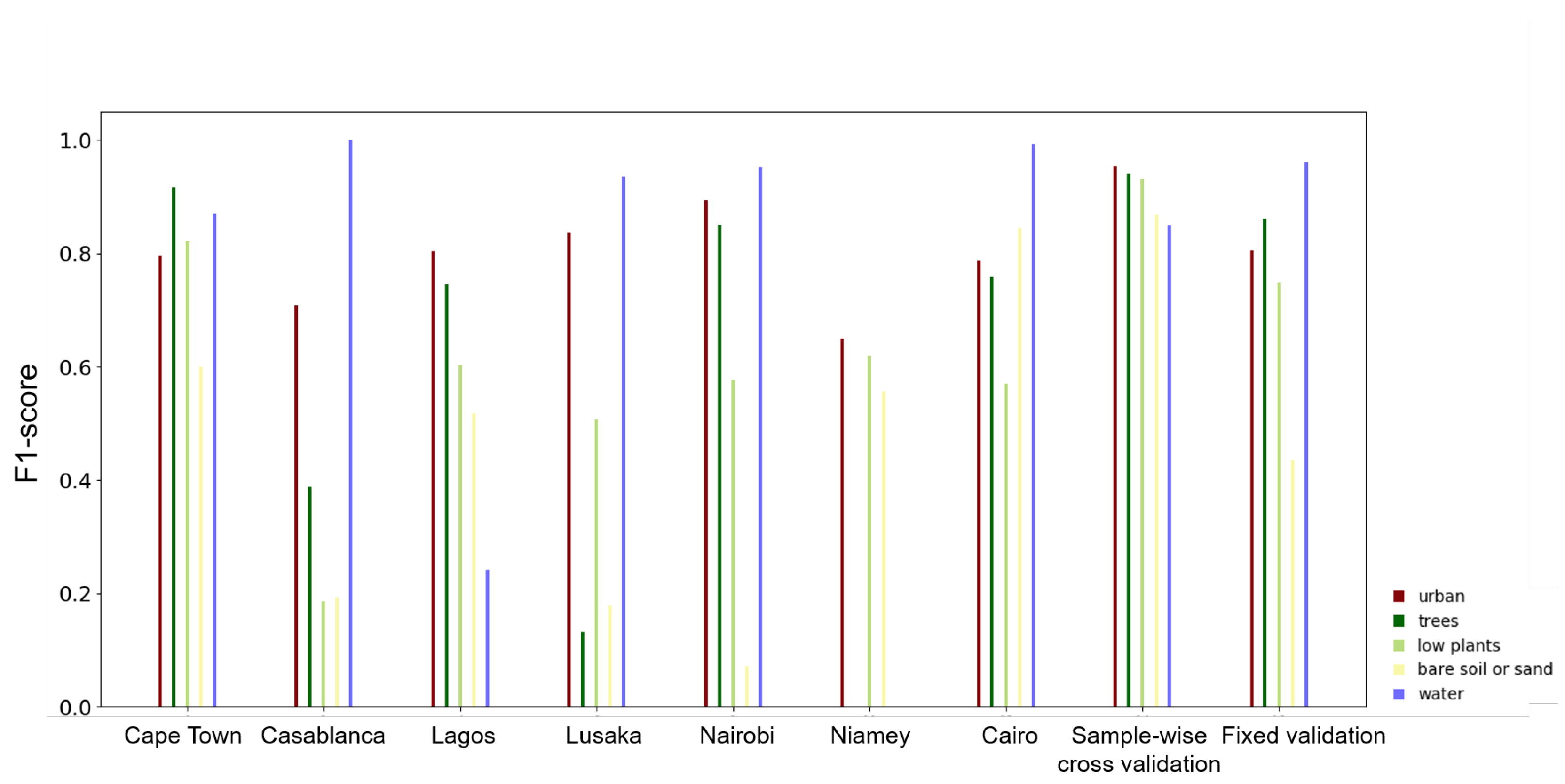
  • City-wise holdout cross validation: The reference samples from six training cities are used for training models and samples from the one remaining city are used for testing models. Since there are seven cities, this classification procedure was performed seven times. In this case, the information for training is independent of that used for testing, which facilitates the assessment of transferability of the trained models for each land cover class across different areas.
  • Sample-wise cross validation: All training samples are randomly split into five folds, where four folds of class samples that include data from all the training cities are fed to the classifier and the remaining fold of class samples is used for testing. This experiment is used for comparison and provides an upper bound for mapping accuracy.

4. Results

4.1. Comparative Classification Accuracy of Different Input Configurations

Based on the training samples collected from all seven training cities, we compare the classification accuracy of different input configurations validated on two evaluation cities, which are listed in Table 4. It is observed that there is always an increase of accuracy when new data are introduced, so that the highest accuracy (OA = 0.8105, Kappa = 0.7602) is achieved when all available datasets are included.
Figure 4 shows the relative importance of the different input features, which is derived from the RF importance analysis implementation in Python’s Scikit-learn library. Some spectral indices show higher importance than other configurations. Figure 5 illustrates the pixel values for two features (NDVI and MNDWI from Sentinel-2) for each land cover class in all training cities, arranged by latitude. In order to distinguish different land cover classes, the same land cover class in different cities should have as similar a range as possible. It can be seen that natural land cover classes such as trees and low plants have high values of NDVI, while these values for the water and urban classes are low. Similarly, the MNDWI value of most water samples is higher than for other land cover classes.

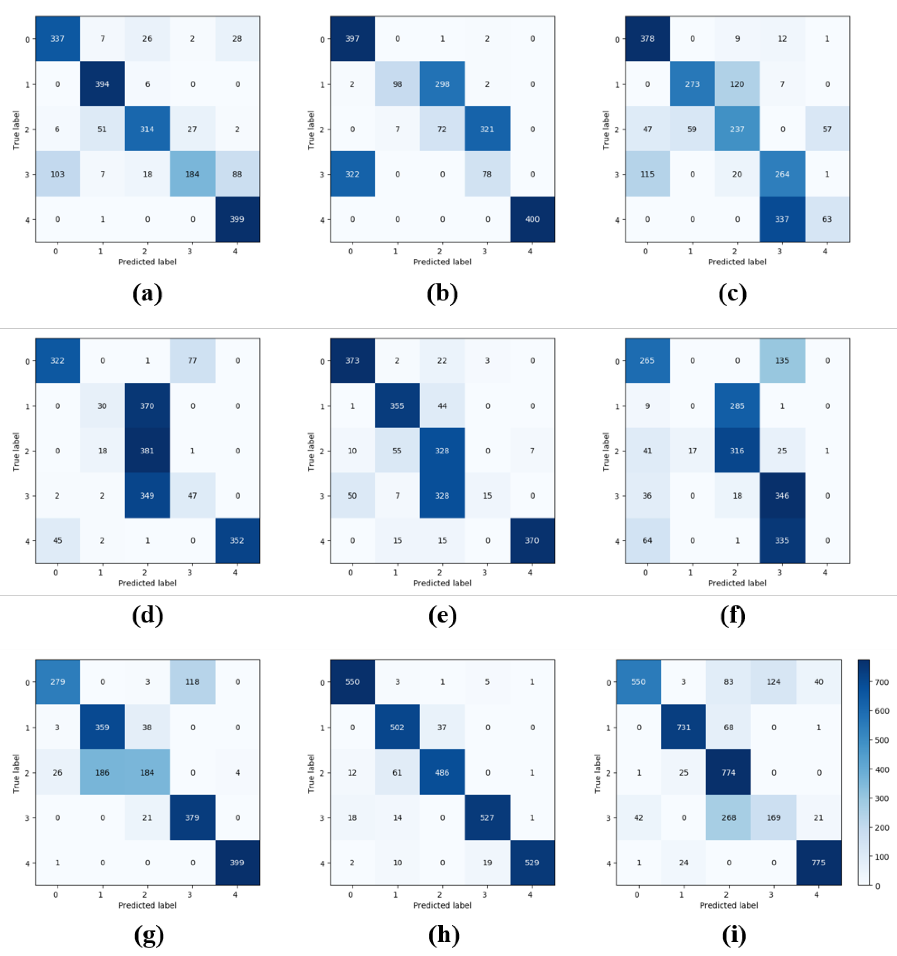
4.2. Transferability of Trained Models

After the selection of best input configurations, the experiments of “city-wise holdout cross validation” and “sample-wise cross validation” are carried out in order to investigate the transferability of the trained models. The accuracy values are listed in Table 5. “Fixed validation” represents the model trained on all seven training cities and tested on the two evaluation cities. “City-wise holdout cross validation” means that the trained model is derived from six training cities and applied to one remaining training city. The city name indicates that the model is trained on the other six cities and tested on this city. In the “sample-wise cross validation”, four folds of all class samples across all training cities are trained and one fold of the samples of the training cities is used for evaluation.
Figure 6 compares the F1-score obtained from different trained models. Confusion tables of all experiments are illustrated in Figure 7 in order to explain the reasons for the low F1-score of a certain land cover class in each cross validation experiment. For the experiments of “city-wise holdout cross validation”, there is a huge difference in the accuracy indices among the seven cities. The OA of three cities exceed 0.7: Capetown, Cairo, and Nairobi, which achieved OA at 0.8140, 0.8000, and 0.7205, respectively. The results of the other four cities are slightly lower, due to the many misclassifications among the five land cover classes. The land cover maps and their corresponding Google Earth imagery of these four cities are shown in Figure 8.

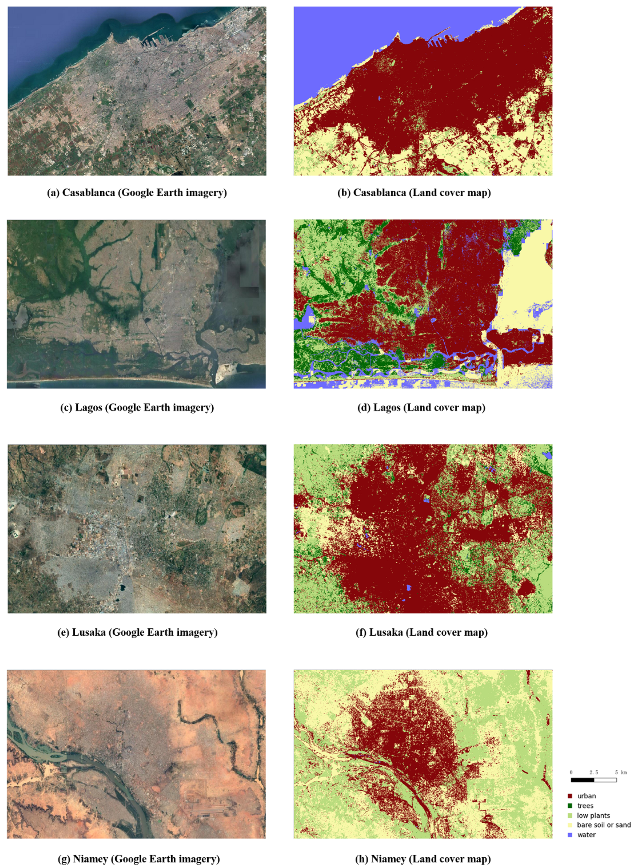
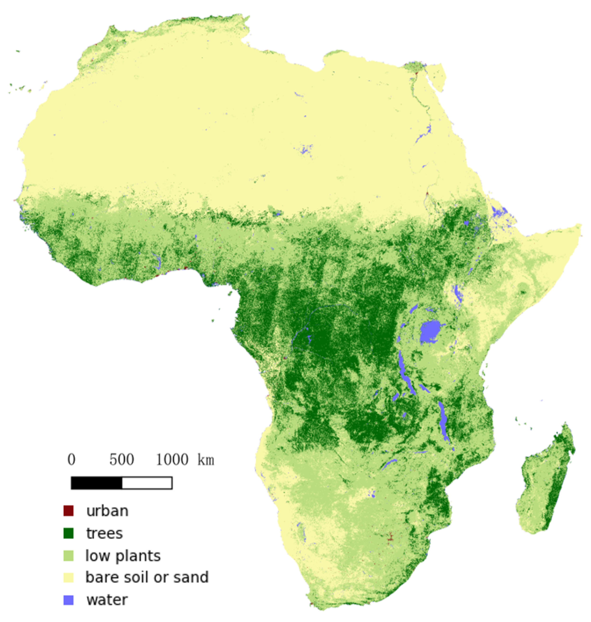
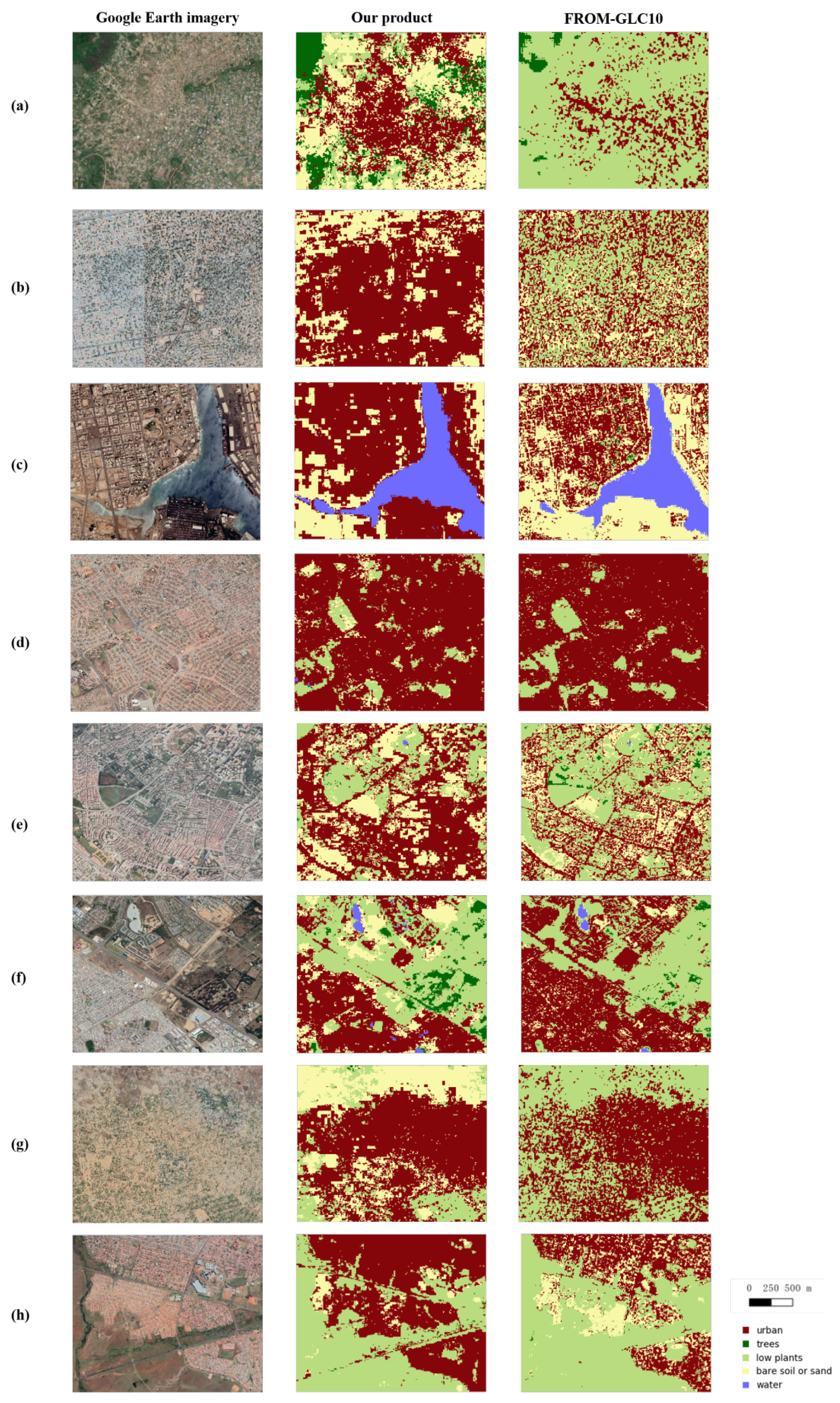
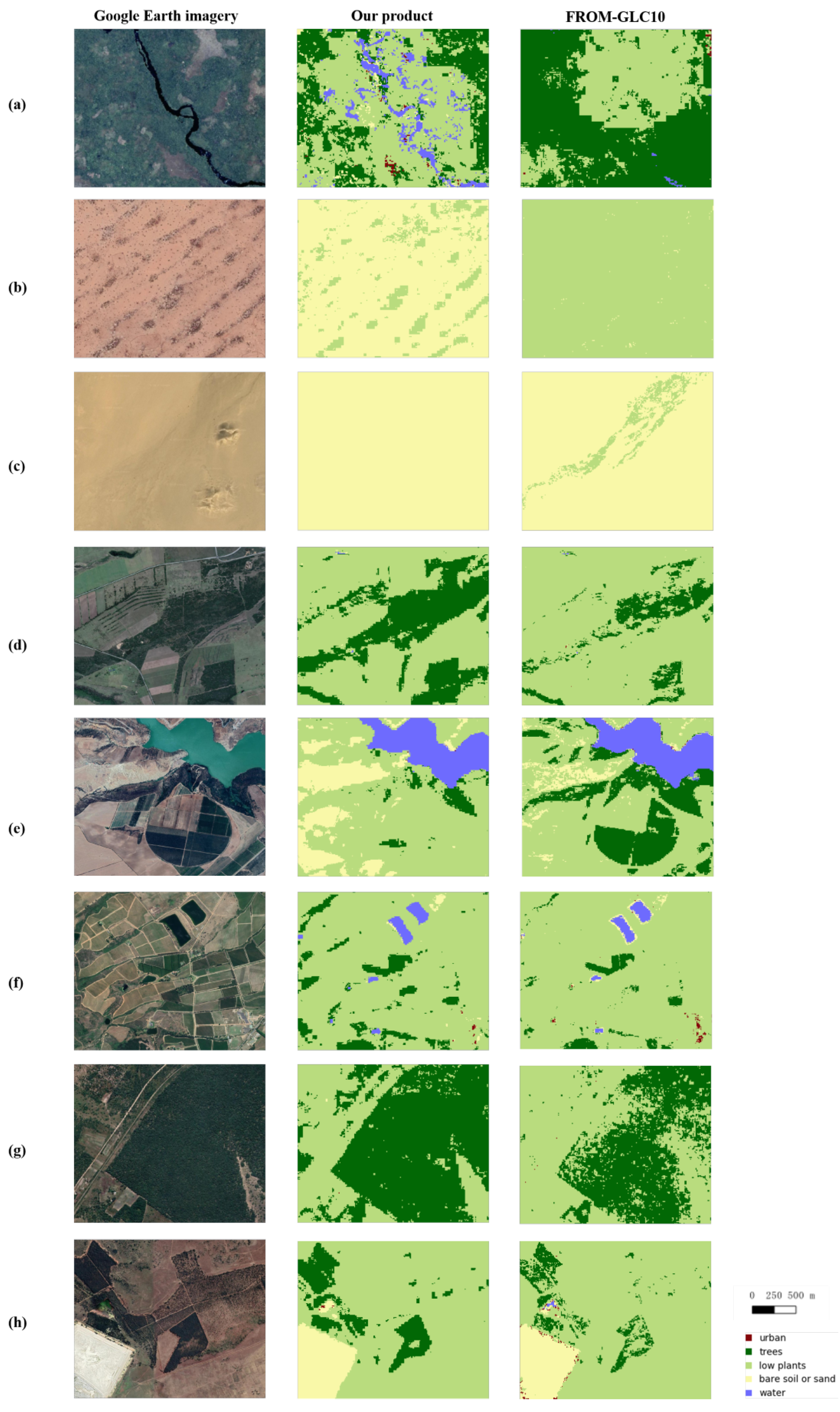
4.3. Land Cover Map of the Whole African Continent

The land cover map of the whole African continent from the best input configurations is illustrated in Figure 9. Land cover maps of the urban and rural regions in each climate zone are shown in Figure 10 and Figure 11, respectively. In order to make a better comparison between our product and FROM-GLC10, we redefine the classification system of FROM-GLC10, where the class of impervious surface, forest, water, and bare land in FROM-GLC10 correspond to urban, trees, water, and bare soil/sand in our product, respectively. The classes of cropland, grassland, shrubland, wetland, and tundra in FROM-GLC10 product correspond to the class of low plants in our product. From the visual results, there is nearly no salt–pepper effect on our product, but FROM-GLC10 shows some noise in certain areas. This superiority of our product lies in the incorporation of multi-source data such as GHSL and NTL in our proposed framework, which provides complementary information to separate between different classes. The urban class in the city area is better captured by our product compared to FROM-GLC10. For example, the area in Figure 10c,h is mainly covered by urban, which is wrongly classified as bare soil/sand in FROM-GLC10. This may be due to the fact that our proposed framework utilizes GHSL and NTL, which could be beneficial to the recognition of urban areas. In most rural regions of Africa, the interlaced distribution of trees and low plants increases the difficulty of satellite-based land cover mapping. However, the transition between trees and low plants is closer to the real land surface in our product than that in FROM-GLC10, according to the high-resolution images from Google Earth (see Figure 11d,g). The water in Figure 11a has been detected in our product, but not identified in the FROM-GLC10 product. In Figure 11b, most of the land is covered by bare soil or sand and low plants, which are better discerned by our product than by FROM-GLC10. Figure 11c is a desert area covered by only bare soil or sand, however, FROM-GLC10 has resulted in some confusion between bare soil or sand and low plants. The cropland in Figure 11e is accurately recognized as low plants in our product, while is misclassified as trees in FROM-GLC10. The temporal consistency and more fine-grained details of our training samples are more beneficial to the discrimination among natural land cover classes. More specifically, the training samples in our product are collected within a 10 m × 10 m area using Google Earth high-resolution imagery acquired in 2017. However, when producing FROM-GLC10, training set was collected with a sample unit (from 30 m × 30 m to 500 m × 500 m) corresponding to Landsat-8 images acquired in 2014 and 2015. Moreover, our research is concentrated on Africa, while the focus of FROM-GLC10 is the global world rather than only Africa. In this case, FROM-GLC10 needs a more generalized model for the global world, which may lead to some discrepancies in Africa.

5. Discussion

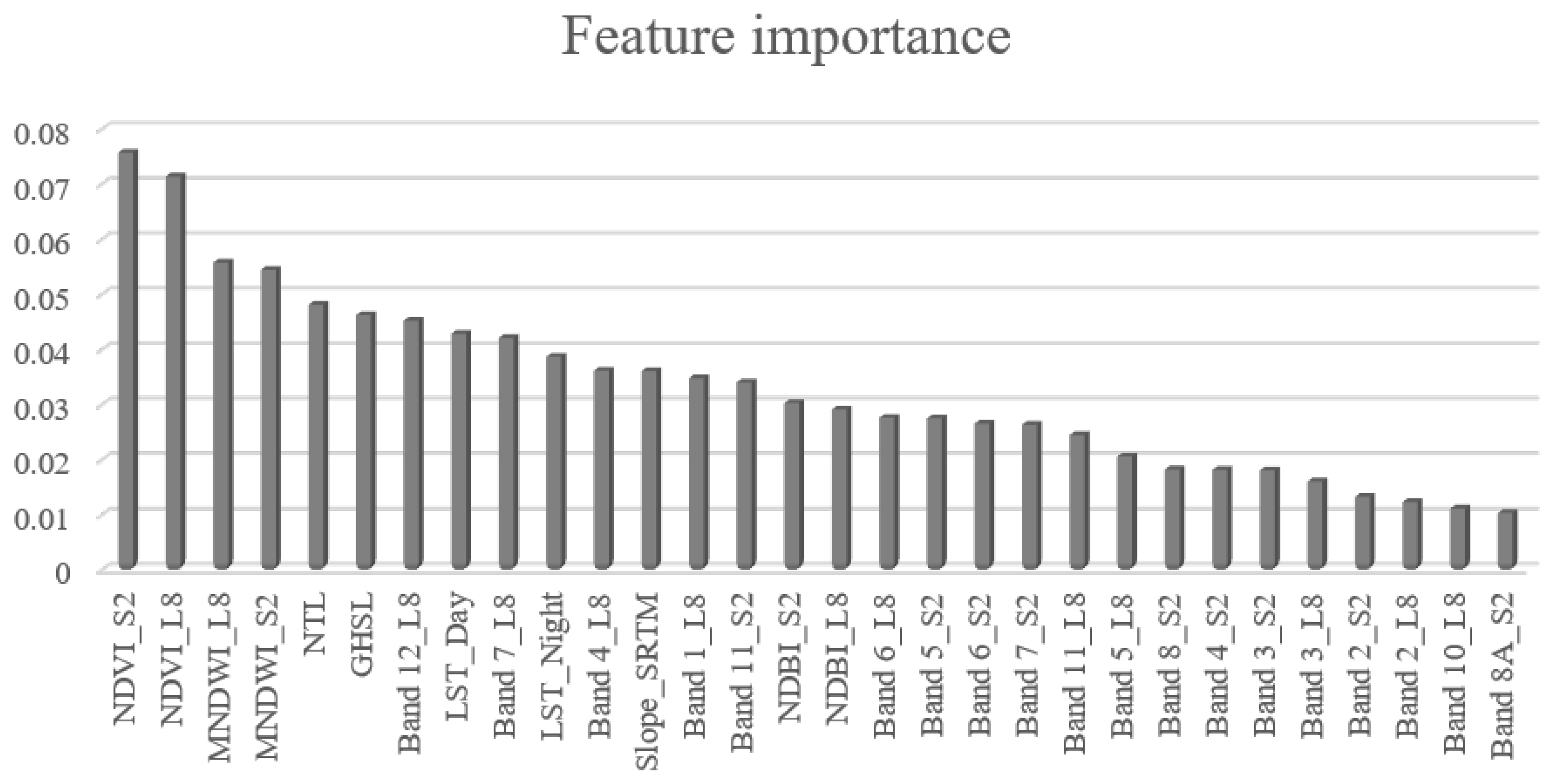
5.1. Input Configurations Analysis

It is observed that the overall accuracy trends (Table 4) and the feature importance (Figure 4) are consistent. The datasets under consideration such as GHSL, NTL, LST, and SRTM, all have high importance, which also contribute to the improvement of classification accuracy when introduced as input configurations. As the first input configuration, the spectral bands of Sentinel-2 provide a variety of spectral information, which contribute to the whole classification. After the spectral indices are introduced, the accuracy indices are improved. Specifically, the NDVI from Sentinel-2 (NDVI_S2) is found to have the highest importance scores, followed by MNDWI from Sentinel-2 (MNDWI_S2). On the one hand, spectral indices combine different spectral bands, which indicates the relative abundance of certain land cover classes. For instance, NDVI is the most common vegetation indice to separate the vegetation and non-vegetation classes, and NDBI is a built-up index helpful for mapping built-up areas. Open water can be delineated by water index (MNDWI). On the other hand, atmospheric effects could also be compensated by utilizing spectral indices.
It is understandable that different datasets have different capabilities in recognizing some land cover classes, which facilitate the improvement the overall classification accuracy [50]. The wavelength range of spectral bands between Landsat-8 and Sentinel-2 is slightly different, and thus, Landsat-8 will provide alternative spectral information that discriminates among land cover classes. GHSL provides the spatial distribution of built-up structures, which supports the identification of urban area. NTL, which has captured artificial lighting, signifies the urban areas. Since different land cover classes are characterized by varying geographic conditions, the DEM and temperature information obtained from SRTM and LST data are also beneficial to the classification.

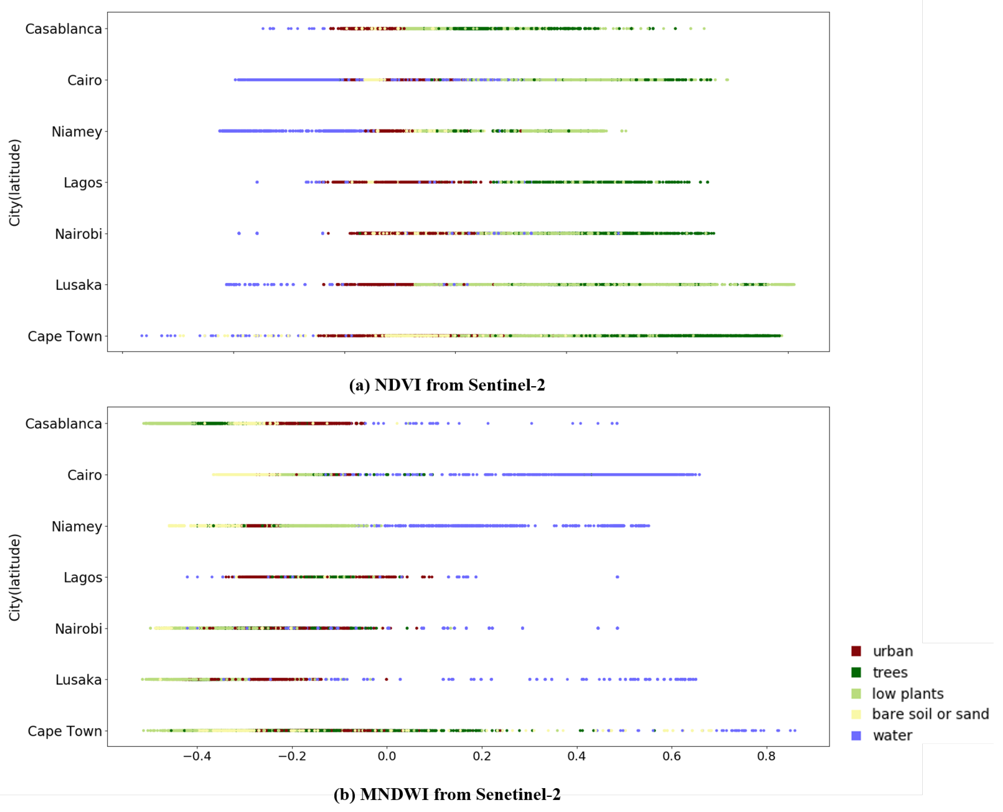
5.2. Transferability Analysis of Trained Models for Each Land Cover Class across Different Cites

The highest accuracy indices are achieved by the experiment of “sample-wise cross validation”, which is not only related to spatial proximity between training samples and testing samples, but also due to the fact that the training set and test set are sampled from the same distribution. The results of the “city-wise holdout cross validation” are generally poor when compared to those of the “sample-wise cross validation”, due to several issues: (1) The trained model might be overfitting to the training data; (2) the training samples are not reliable enough to cover all possible target data; and (3) the difficulty of discriminating among different land cover classes across different cities. For instance, the lower accuracy of Casablanca resulted from the relatively lower transferability of some natural land cover classes such as bare soil or sand and low plants. The reason is that the advantageous geographical conditions of Casablanca such as terrain and climate offer a good opportunity for the development of agriculture. Therefore, there is a lot of agricultural land (belongs to the “low plants” class) in the city area, which is different from the other six cities. For an input configuration to be relevant across cities, the value range of the same land cover class should be as similar as possible for each city. In order to distinguish between different land cover classes, the value range of different land cover classes should be as different as possible. However, from Figure 5, it is clearly seen that even the input configuration with highest importance is not enough for land cover classification across different cities. These issues could be addressed by aiming at less powerful local models, which means that site-specific training sample collection and model training are the best way of generating a land cover map for a city of interest. However, this approach takes a significant amount of time and manual work, which is not feasible for large-scale land cover mapping. The experiment of “city-wise holdout cross validation” is a more realistic test for the transferability of trained models, which could be exploited to upscale existing training for continental or global scale land cover maps.
The transferability of trained models for the urban class holds great potential in African land cover mapping. From Figure 6, it is apparent that the urban class of all cities exceeds the threshold of 0.6 for F1-score. It is hypothesized that these cities have similar spectral signatures due to their similar urban morphologies [20], which are related to the infrastructure and housing in a city. In most African cities, a lower proportion of central land is dedicated to transport use, such as paved roads, and this proportion rapidly declines near the edges of the city [51]. Moreover, a great many African cities are characterized by low-rise buildings [52], and much land within the central business district remains unbuilt [53]. This is due to unclear ownership of land and insufficient financing [54]. In this regard, the trained models for the urban class could be easily transferred to the whole continent of Africa, which indicates good reusability of urban samples in the land cover mapping of the whole African continent.
However, for the natural land cover classes such as trees, low plants, bare soil or sand, and water, they are more difficult to transfer the trained models across different cities. In this regard, all representative samples should be considered during the process of training sample selection for natural land cover classes, which could provide the basis for intelligent transfers between cities. For instance, the results for the tree class are not satisfactory for Casablanca, Lusaka, and Niamey, which indicates that the tree class in these three cities are largely different from other cities. In particular, the lowest F1-score of trees exists in the Niamey experiment. It can be seen from the confusion matrix (Figure 7f) and visual result (Figure 8h) of Niamey that almost all trees are misclassified as low plants. More than 90% of the trees within the Niamey are the Neem species [55], a tree that is mainly located in semi-arid areas. Thus, the training samples of trees collected from the other six cities are unable to discriminate trees from low plants in Niamey. Moreover, the F1-score of the water class is also the lowest in Niamey. The largest water body in Niamey is the Niger River, which flows across the city from the northwest to the southeast. In these areas, there is great confusion between water and other classes such as urban and soil/sand, which results from the high sediment content in the water. Therefore, when we select the water samples, the water samples should cover not only oceans, but also lakes and rivers that may have different sediment contents. In this regard, the quality and quantity of training samples will be improved.

5.3. Implication of Our African Land Cover Map

The information of five land cover classes from our product is essential for a better understanding of many of the Earth’s land surface processes. For instance, the information on the “urban” class can allow for monitoring trends in urbanization [56] and provide a large-scale base layer for a more detailed local climate zone mapping of urban areas [57], which lie in the focus of interest of many studies. The “trees” class and “low plants” class are vegetation, which plays a critical role in improving performances of the ecosystem, thus, this information is beneficial to investigate carbon cycling [58]. Water has a close relation to climate, biological diversity, and human wellbeing. In this regard, the “water” class provides information for water-management decision-making [59]. The transition from vegetation to the “bare soil or sand” class is helpful to understand the status of and tracking desertification [60]. Moreover, the combination of “urban” class, “trees” class, and “low plants” class in the city could be exploited to assess the impacts of urban form on the landscape structure of urban green spaces [61].
In addition, a local climate zone classification map with more land cover classes could also be derived from our product after further processing. In the local climate zone classification scheme [33], “dense trees” is defined as the heavily wooded landscape of trees, and “scattered trees” represents the lightly wooded landscape of trees on the pervious area (low plants). In this case, the ratios of different land cover classes within a block (100 m × 100 m) could be firstly calculated. According to these ratios, the new land cover class label could be assigned to each block. For instance, if the ratio of the “trees” class is dominant in this block, then we can assign this block with “dense trees” class. When the “trees” class and “low plants” class have the largest two and similar ratios, this block could be classified as “scattered trees”. In this regard, the newly generated local climate zone classification map provides auxiliary data for applications such as urban climate studies [62] and urban planning [63].

6. Conclusions

Given that GEE is an efficient platform for large-scale and multi-source data processing and analysis, we have proposed a framework for African land cover mapping at 10 m from multi-source data with GEE, and demonstrated its effectiveness for large-scale land cover mapping. Especially, a large-scale base layer could be acquired from our product for a more detailed local climate zone mapping of urban areas in the future work. In this regard, our land cover maps of 30 sample African cities are released and users can access it through the link: https://drive.google.com/open?id=1_x2YCFqCk7eEp0jc1v83-E_uxYOhIEYU. This new 10-m resolution dataset could be utilized for further applications by researchers from all around the world. We will continuously update and refine this dataset in the future. Our product has better captured some land cover types than FROM-GLC10 does, an existing global land cover map at 10 m. Specifically, the urban class is better extracted in city areas and the transition between trees and low plants is closer to the real land surface in rural areas. This may be due to the combination of more multi-source data in our proposed framework, which indicates the importance of multi-source data for improving land cover classification accuracy at extensive scales, e.g., for whole continents.
Within the proposed mapping framework, a number of multi-source data are selected to generate land cover maps. We have evaluated the characteristics and performances of different input configurations by a comparison of their land cover classification results. The use of all considered multi-source data, which include Sentinel-2, Landsat-8, GHSL, NTL, SRTM, and LST, has achieved the best capability for land cover classification.
In addition, the transferability of trained models for each land cover class across different cities is investigated here in continental land cover mapping tasks for the first time. The experiments of “city-wise hold out cross validation” in this study demonstrates that the transferability of trained models for the urban class is much better than other natural land cover classes such as trees, low plants, and water. Therefore, it is suggested that training samples of natural land cover classes should be collected from areas covering each main Köppen climate zone for African land cover mapping and other similar tasks. It is a vital outcome, which denotes that this sampling strategy, which covers areas in all the different Köppen climate zones, could support better upscaling to continental levels.

Author Contributions

Conceptualization, X.X.Z. and M.S.; methodology, Q.L. and C.Q.; software, Q.L. and C.Q.; validation, Q.L.; formal analysis, Q.L., C.Q. and L.M.; investigation, Q.L.; resources, X.X.Z.; data curation, Q.L. and C.Q.; writing—original draft preparation, Q.L.; writing—review and editing, Q.L., C.Q., L.M. and M.S.; visualization, Q.L.; supervision, X.X.Z.; project administration, X.X.Z.; funding acquisition, X.X.Z. All authors have read and agreed to the published version of the manuscript.

Funding

This work is supported by the European Research Council (ERC) under the European Union’s Horizon 2020 research and innovation programme (grant agreement no. ERC-2016-StG-714087, acronym: So2Sat, www.so2sat.eu), the Helmholtz Association under the framework of the Young Investigators Group “SiPEO” (VH-NG-1018, www.sipeo.bgu.tum.de) and Helmholtz Excellent Professorship “Data Science in Earth Observation—Big Data Fusion for Urban Research”.

Conflicts of Interest

The authors declare no conflict of interest. The founding sponsors had no role in the design of the study; in the collection, analyses, or interpretation of data; in the writing of the manuscript, and in the decision to publish the results.

References

  1. Friedl, M.A.; Sulla-Menashe, D.; Tan, B.; Schneider, A.; Ramankutty, N.; Sibley, A.; Huang, X. MODIS Collection 5 global land cover: Algorithm refinements and characterization of new datasets. Remote Sens. Environ. 2010, 114, 168–182. [Google Scholar] [CrossRef]
  2. Arino, O.; Bicheron, P.; Achard, F.; Latham, J.; Witt, R.; Weber, J.L. The most detailed portrait of Earth. Eur. Space Agency 2008, 136, 25–31. [Google Scholar]
  3. Hansen, M.C.; DeFries, R.S.; Townshend, J.R.; Sohlberg, R. Global land cover classification at 1 km spatial resolution using a classification tree approach. Int. J. Remote Sens. 2000, 21, 1331–1364. [Google Scholar] [CrossRef]
  4. Bontemps, S.; Defourny, P.; Radoux, J.; Van Bogaert, E.; Lamarche, C.; Achard, F.; Mayaux, P.; Boettcher, M.; Brockmann, C.; Kirches, G.; et al. Consistent global land cover maps for climate modelling communities: Current achievements of the ESA’s land cover CCI. In Proceedings of the ESA Living Planet Symposium, Edinburgh, UK, 9–13 September 2013; pp. 9–13. [Google Scholar]
  5. Latham, J.; Cumani, R.; Rosati, I.; Bloise, M. Global Land Cover Share (GLC-SHARE) Database Beta-Release Version 1.0-2014; FAO: Rome, Italy, 2014. [Google Scholar]
  6. Tateishi, R.; Uriyangqai, B.; Al-Bilbisi, H.; Ghar, M.A.; Tsend-Ayush, J.; Kobayashi, T.; Kasimu, A.; Hoan, N.T.; Shalaby, A.; Alsaaideh, B.; et al. Production of global land cover data–GLCNMO. Int. J. Digit. Earth 2011, 4, 22–49. [Google Scholar] [CrossRef]
  7. Copernicus Global Land Service. Providing Bio-Geophysical Products of Global Land Surface. Available online: https://land.copernicus.eu/global/index.html (accessed on 12 June 2018).
  8. Gong, P.; Liu, H.; Zhang, M.; Li, C.; Wang, J.; Huang, H.; Clinton, N.; Ji, L.; Li, W.; Bai, Y.; et al. Stable classification with limited sample: Transferring a 30-m resolution sample set collected in 2015 to mapping 10-m resolution global land cover in 2017. Sci. Bull. 2019, 64, 370–373. [Google Scholar] [CrossRef] [Green Version]
  9. Gong, P.; Wang, J.; Yu, L.; Zhao, Y.; Zhao, Y.; Liang, L.; Niu, Z.; Huang, X.; Fu, H.; Liu, S.; et al. Finer resolution observation and monitoring of global land cover: First mapping results with Landsat TM and ETM+ data. Int. J. Remote Sens. 2013, 34, 2607–2654. [Google Scholar] [CrossRef] [Green Version]
  10. Chen, J.; Chen, J.; Liao, A.; Cao, X.; Chen, L.; Chen, X.; He, C.; Han, G.; Peng, S.; Lu, M.; et al. Global land cover mapping at 30 m resolution: A POK-based operational approach. ISPRS J. Photogramm. Remote Sens. 2015, 103, 7–27. [Google Scholar] [CrossRef] [Green Version]
  11. Gorelick, N.; Hancher, M.; Dixon, M.; Ilyushchenko, S.; Thau, D.; Moore, R. Google Earth Engine: Planetary-scale geospatial analysis for everyone. Remote Sens. Environ. 2017, 202, 18–27. [Google Scholar] [CrossRef]
  12. Huang, H.; Chen, Y.; Clinton, N.; Wang, J.; Wang, X.; Liu, C.; Gong, P.; Yang, J.; Bai, Y.; Zheng, Y.; et al. Mapping major land cover dynamics in Beijing using all Landsat images in Google Earth Engine. Remote Sens. Environ. 2017, 202, 166–176. [Google Scholar] [CrossRef]
  13. Sidhu, N.; Pebesma, E.; Câmara, G. Using Google Earth Engine to detect land cover change: Singapore as a use case. Eur. J. Remote Sens. 2018, 51, 486–500. [Google Scholar] [CrossRef]
  14. Carrasco, L.; O’Neil, A.W.; Morton, R.D.; Rowland, C.S. Evaluating combinations of temporally aggregated Sentinel-1, Sentinel-2 and Landsat 8 For land cover mapping with Google Earth Engine. Remote Sens. 2019, 11, 288. [Google Scholar] [CrossRef] [Green Version]
  15. Qiu, C.; Schmitt, M.; Geiss, C.; Chen, T.K.; Zhu, X.X. A framework for large-scale mapping of human settlement extent from Sentinel-2 images via fully convolutional neural networks. arXiv 2020, arXiv:2001.11935. [Google Scholar]
  16. Steinmann, G. Population, Resources, and Limits to Growth. In Development Economics: Theory, Practice, and Prospects; Springer: Dordrecht, The Netherlands, 1989; pp. 87–128. [Google Scholar]
  17. Reich, P.; Numbem, S.; Almaraz, R.; Eswaran, H. Land resource stresses and desertification in Africa. Agro-Science 2001, 2, 2. [Google Scholar]
  18. Midekisa, A.; Holl, F.; Savory, D.J.; Andrade-Pacheco, R.; Gething, P.W.; Bennett, A.; Sturrock, H.J. Mapping land cover change over continental Africa using Landsat and Google Earth Engine cloud computing. PLoS ONE 2017, 12, e0184926. [Google Scholar] [CrossRef]
  19. Schmitt, M.; Zhu, X.X. Data fusion and remote sensing: An ever-growing relationship. IEEE Geosci. Remote Sens. Mag. 2016, 4, 6–23. [Google Scholar] [CrossRef]
  20. Demuzere, M.; Bechtel, B.; Mills, G. Global transferability of local climate zone models. Urban Clim. 2019, 27, 46–63. [Google Scholar] [CrossRef]
  21. Gatti, A.; Bertolini, A. Sentinel-2 Products Specification Document. 2013. Available online: https://earth.esa.int/documents/247904/685211/Sentinel-2+Products+Specification+Document (accessed on 23 February 2015).
  22. Roy, D.P.; Wulder, M.A.; Loveland, T.R.; Woodcock, C.; Allen, R.G.; Anderson, M.C.; Helder, D.; Irons, J.R.; Johnson, D.M.; Kennedy, R.; et al. Landsat-8: Science and product vision for terrestrial global change research. Remote Sens. Environ. 2014, 145, 154–172. [Google Scholar] [CrossRef] [Green Version]
  23. Elvidge, C.D.; Baugh, K.E.; Zhizhin, M.; Hsu, F.C. Why VIIRS data are superior to DMSP for mapping nighttime lights. Proc. Asia-Pac. Adv. Netw. 2013, 35, 62. [Google Scholar] [CrossRef] [Green Version]
  24. Pesaresi, M.; Ehrilch, D.; Florczyk, A.J.; Freire, S.; Julea, A.; Kemper, T.; Soille, P.; Syrris, V. GHS Built-Up Grid, Derived from Landsat, Multitemporal (1975, 1990, 2000, 2014). European Commission; Joint Research Centre (JRC)[Dataset] PID: 2015. Available online: http://data.europa.eu/89h/jrc-ghsl-ghs_built_ldsmt_globe_r2015b (accessed on 10 January 2020). (In Luxembourg).
  25. Farr, T.G.; Rosen, P.A.; Caro, E.; Crippen, R.; Duren, R.; Hensley, S.; Kobrick, M.; Paller, M.; Rodriguez, E.; Roth, L.; et al. The shuttle radar topography mission. Rev. Geophys. 2007, 45, 2. [Google Scholar] [CrossRef] [Green Version]
  26. Wan, Z.; Hook, S.; Hulley, G. MYD11A2 MODIS/Aqua Land Surface Temperature/Emissivity 8-Day L3 Global 1 km SIN Grid V006. 2015, Distributed by NASA EOSDIS Land Processes DAAC. Available online: https://doi.org/10.5067/MODIS/MYD11A2.006 (accessed on 23 June 2019).
  27. Foga, S.; Scaramuzza, P.L.; Guo, S.; Zhu, Z.; Dilley, R.D., Jr.; Beckmann, T.; Schmidt, G.L.; Dwyer, J.L.; Hughes, M.J.; Laue, B. Cloud detection algorithm comparison and validation for operational Landsat data products. Remote Sens. Environ. 2017, 194, 379–390. [Google Scholar] [CrossRef] [Green Version]
  28. Braaten, J.D.; Cohen, W.B.; Yang, Z. Automated cloud and cloud shadow identification in Landsat MSS imagery for temperate ecosystems. Remote Sens. Environ. 2015, 169, 128–138. [Google Scholar] [CrossRef] [Green Version]
  29. Zha, Y.; Gao, J.; Ni, S. Use of normalized difference built-up index in automatically mapping urban areas from TM imagery. Int. J. Remote Sens. 2003, 24, 583–594. [Google Scholar] [CrossRef]
  30. Rouse, J., Jr.; Haas, R.; Schell, J.; Deering, D. Monitoring Vegetation Systems in the Great Plains with ERTS; NASA Special Publication: Washington, DC, USA, 1974.
  31. Xu, H. Modification of normalised difference water index (NDWI) to enhance open water features in remotely sensed imagery. Int. J. Remote Sens. 2006, 27, 3025–3033. [Google Scholar] [CrossRef]
  32. Jhonnerie, R.; Siregar, V.P.; Nababan, B.; Prasetyo, L.B.; Wouthuyzen, S. Random forest classification for mangrove land cover mapping using Landsat 5 TM and ALOS PALSAR imageries. Procedia Environ. Sci. 2015, 24, 215–221. [Google Scholar] [CrossRef] [Green Version]
  33. Stewart, I.D.; Oke, T.R. Local climate zones for urban temperature studies. Bull. Am. Meteorol. Soc. 2012, 93, 1879–1900. [Google Scholar] [CrossRef]
  34. Stewart, I.D.; Oke, T.R.; Krayenhoff, E.S. Evaluation of the ‘local climate zone’scheme using temperature observations and model simulations. Int. J. Climatol. 2014, 34, 1062–1080. [Google Scholar] [CrossRef]
  35. Peel, M.C.; Finlayson, B.L.; McMahon, T.A. Updated world map of the Köppen-Geiger climate classification. Hydrol. Earth Syst. Sci. Discuss. 2007, 4, 439–473. [Google Scholar] [CrossRef] [Green Version]
  36. Rikimaru, A. Development of forest canopy density mapping and monitoring model using indices of vegetation, bare soil and shadow. In Proceedings of the 18th ACRS, Kuala Lumpur, Malaysia, 20–24 October 1997. [Google Scholar]
  37. Breiman, L. Random forests. Mach. Learn. 2001, 45, 5–32. [Google Scholar] [CrossRef] [Green Version]
  38. Schneider, A. Monitoring land cover change in urban and peri-urban areas using dense time stacks of Landsat satellite data and a data mining approach. Remote Sens. Environ. 2012, 124, 689–704. [Google Scholar] [CrossRef]
  39. Hu, Y.; Hu, Y. Land Cover Changes and Their Driving Mechanisms in Central Asia from 2001 to 2017 Supported by Google Earth Engine. Remote Sens. 2019, 11, 554. [Google Scholar] [CrossRef] [Green Version]
  40. Belgiu, M.; Drăguţ, L. Random forest in remote sensing: A review of applications and future directions. ISPRS J. Photogramm. Remote Sens. 2016, 114, 24–31. [Google Scholar] [CrossRef]
  41. Li, Q.; Huang, X.; Wen, D.; Liu, H. Integrating multiple textural features for remote sensing image change detection. Photogramm. Eng. Remote Sens. 2017, 83, 109–121. [Google Scholar] [CrossRef]
  42. Ma, L.; Li, M.; Ma, X.; Cheng, L.; Du, P.; Liu, Y. A review of supervised object-based land-cover image classification. ISPRS J. Photogramm. Remote Sens. 2017, 130, 277–293. [Google Scholar] [CrossRef]
  43. Li, M.; Ma, L.; Blaschke, T.; Cheng, L.; Tiede, D. A systematic comparison of different object-based classification techniques using high spatial resolution imagery in agricultural environments. Int. J. Appl. Earth Obs. Geoinf. 2016, 49, 87–98. [Google Scholar] [CrossRef]
  44. Ma, L.; Fu, T.; Blaschke, T.; Li, M.; Tiede, D.; Zhou, Z.; Ma, X.; Chen, D. Evaluation of feature selection methods for object-based land cover mapping of unmanned aerial vehicle imagery using random forest and support vector machine classifiers. ISPRS Int. J. Geo-Inf. 2017, 6, 51. [Google Scholar] [CrossRef]
  45. Foody, G.M. Status of land cover classification accuracy assessment. Remote Sens. Environ. 2002, 80, 185–201. [Google Scholar] [CrossRef]
  46. Melchiorri, M.; Florczyk, A.; Freire, S.; Schiavina, M.; Pesaresi, M.; Kemper, T. Unveiling 25 years of planetary urbanization with remote sensing: Perspectives from the global human settlement layer. Remote Sens. 2018, 10, 768. [Google Scholar] [CrossRef] [Green Version]
  47. Huang, X.; Li, Q.; Liu, H.; Li, J. Assessing and improving the accuracy of GlobeLand30 data for urban area delineation by combining multisource remote sensing data. IEEE Geosci. Remote Sens. Lett. 2016, 13, 1860–1864. [Google Scholar] [CrossRef]
  48. Na, X.; Zhang, S.; Li, X.; Yu, H.; Liu, C. Improved land cover mapping using random forests combined with landsat thematic mapper imagery and ancillary geographic data. Photogramm. Eng. Remote Sens. 2010, 76, 833–840. [Google Scholar] [CrossRef]
  49. Bounoua, L.; DeFries, R.; Collatz, G.J.; Sellers, P.; Khan, H. Effects of land cover conversion on surface climate. Clim. Chang. 2002, 52, 29–64. [Google Scholar] [CrossRef]
  50. Khatami, R.; Mountrakis, G.; Stehman, S.V. A meta-analysis of remote sensing research on supervised pixel-based land-cover image classification processes: General guidelines for practitioners and future research. Remote Sens. Environ. 2016, 177, 89–100. [Google Scholar] [CrossRef] [Green Version]
  51. Antos, S.E.; Lall, S.V.; Lozano-Gracia, N. The Morphology of African Cities; The World Bank: Washington, DC, USA, 2016. [Google Scholar]
  52. Ede, A.N. Challenges Affecting the Development and Optimal Use of Tall Buildings in Nigeria. Int. J. Eng. Sci. (IJES) 2014, 3, 12–20. [Google Scholar]
  53. Lall, S.V.; Henderson, J.V.; Venables, A.J. Africa’s Cities: Opening Doors to the World; The World Bank: Washington, DC, USA, 2017. [Google Scholar]
  54. Hass, A.; Kopanyi, M. Taxation of Vacant Urban Land: From Theory to Practice; International Growth Center, London School of Economic and Political Science: London, UK, 2017. [Google Scholar]
  55. Abdulazeez, A. A Description of the Physical and Human Geographies of the Niger Republic Capital City, Niamey; Bayero University: Kano, Nigeria, 2015; pp. 2–21. [Google Scholar]
  56. Liu, X.; Hu, G.; Chen, Y.; Li, X.; Xu, X.; Li, S.; Pei, F.; Wang, S. High-resolution multi-temporal mapping of global urban land using Landsat images based on the Google Earth Engine Platform. Remote Sens. Environ. 2018, 209, 227–239. [Google Scholar] [CrossRef]
  57. Qiu, C.; Mou, L.; Schmitt, M.; Zhu, X.X. Local climate zone-based urban land cover classification from multi-seasonal Sentinel-2 images with a recurrent residual network. ISPRS J. Photogramm. Remote Sens. 2019, 154, 151–162. [Google Scholar] [CrossRef] [PubMed]
  58. Poulter, B.; Frank, D.; Hodson, E.; Zimmermann, N. Impacts of land cover and climate data selection on understanding terrestrial carbon dynamics and the CO2 airborne fraction. Biogeosciences 2011, 8, 2027–2036. [Google Scholar] [CrossRef] [Green Version]
  59. Pekel, J.F.; Cottam, A.; Gorelick, N.; Belward, A.S. High-resolution mapping of global surface water and its long-term changes. Nature 2016, 540, 418–422. [Google Scholar] [CrossRef]
  60. Badreldin, N.; Goossens, R. Monitoring land use/land cover change using multi-temporal Landsat satellite images in an arid environment: A case study of El-Arish, Egypt. Arab. J. Geosci. 2014, 7, 1671–1681. [Google Scholar] [CrossRef]
  61. Huang, C.; Yang, J.; Jiang, P. Assessing Impacts of Urban Form on Landscape Structure of Urban Green Spaces in China Using Landsat Images Based on Google Earth Engine. Remote Sens. 2018, 10, 1569. [Google Scholar] [CrossRef] [Green Version]
  62. Kotharkar, R.; Bagade, A. Evaluating urban heat island in the critical local climate zones of an Indian city. Landsc. Urban Plan. 2018, 169, 92–104. [Google Scholar] [CrossRef]
  63. Bechtel, B.; Pesaresi, M.; See, L.; Mills, G.; Ching, J.; Alexander, P.; Feddema, J.; Florczyk, A.; Stewart, I. Towards consistent mapping of urban structure-global human settlement layer and local climate zones. ISPRS-Int. Arch. Photogramm. Remote Sens. Spat. Inf. Sci. 2016, 41, 1371–1378. [Google Scholar] [CrossRef]
Figure 1. Flowchart of the proposed framework.
Remotesensing 12 00602 g001
Figure 2. (a) Study areas: red circles represents training cities, blue circles represents evaluation cities and the distribution of reference samples from (b) Nairobi, and (c) Cape Town.
Remotesensing 12 00602 g002
Figure 3. Number and distribution of each land cover class samples in different cities.
Remotesensing 12 00602 g003
Figure 4. Importance factor of different features. S2 means Sentinel-2, L8 represents Landsat-8.
Remotesensing 12 00602 g004
Figure 5. Meridional profiling of (a) normalized difference vegetation index (NDVI) and (b) modified normalized difference water index (MNDWI) from Sentinel-2 across all training cities, sorted from south (bottom) to north (top). Each pixel is depicted by its input feature value and land cover class.
Remotesensing 12 00602 g005
Figure 6. F1-score of each land cover class in experiments of transferability analysis.
Remotesensing 12 00602 g006
Figure 7. Confusion matrix obtained from the experiments of “city-wise holdout cross validation” with test cities for (a) Cape Town, (b) Casablanca, (c) Lagos, (d) Lusaka, (e) Nairobi, (f) Niamey, (g) Cairo, and (h) “Sample-wise cross validation” as well as (i) “Fixed validation”.
Remotesensing 12 00602 g007
Figure 8. Visual results of experiments of “city-wise holdout cross validation”.
Remotesensing 12 00602 g008
Figure 9. Visual mapping results of the whole continent of Africa.
Remotesensing 12 00602 g009
Figure 10. Google Earth imagery, our product, and the From-CLC10 product of the urban area in the climate zone from (a) Tropical wet climate (Aw), (b) Hot semi-arid climate (BSh), (c) Hot desert climate (BWh), (d) Temperate oceanic climate (Cfb), (e) Hot-summer Mediterranean climate (Csa), (f) Warm-summer Mediterranean climate (Csb), (g) Monsoon-influenced humid subtropical climate (Cwa), and (h) Subtropical highland climate (Cwb).
Remotesensing 12 00602 g010
Figure 11. Google Earth imagery, our product, and the From-CLC10 product of the rural area in the climate zone from (a) Tropical wet climate (Aw), (b) Hot semi-arid climate (BSh), (c) Hot desert climate (BWh), (d) Temperate oceanic climate (Cfb), (e) Hot-summer Mediterranean climate (Csa), (f) Warm-summer Mediterranean climate (Csb), (g) Monsoon-influenced humid subtropical climate (Cwa), and (h) Subtropical highland climate (Cwb).
Remotesensing 12 00602 g011
Table 1. Spectral region and spatial resolution of the bands from Sentinel-2 and Landsat-8.
Sentinel-2Landsat-8
BandSpectral RegionResolution (M)Spectral RegionResolution (M)
Band 1Coastal Aerosol60Coastal Aerosol30
Band 2Blue10Blue30
Band 3Green10Green30
Band 4Red10Red30
Band 5Vegetation red edge120Near Infrared (NIR)30
Band 6Vegetation red edge220Short Wavelength Infrared 1 (SWIR1)30
Band 7Vegetation red edge320Short Wavelength Infrared 2 (SWIR2)30
Band 8NIR10Panchromatic15
Band 8ANarrow Near Infrared20
Band 9Water vapour60Cirrus30
Band 10Cirrus60Thermal Infrared 1 (TIR1)100
Band 11SWIR120Thermal Infrared 2 (TIR2)100
Band 12SWIR120
Table 2. Spectral indices selected for our research.
Spectral IndicesEquation
NDBI N D B I = B a n d S W I R 1 B a n d N I R B a n d S W I R 1 + B a n d N I R
NDVI N D V I = B a n d N I R B a n d R e d B a n d N I R + B a n d R e d
MNDWI M N D W I = B a n d G r e e n B a n d S W I R 1 B a n d G r e e n + B a n d S W I R 1
Table 3. African cities selected for this research.
TypeCityCountryClimate (Köppen Climate Classification)
TrainingCairoEgyptHot desert climate (BWh)
TrainingCape TownSouth AfricaWarm-summer Mediterranean climate (Csb)
TrainingNairobiKenyaTemperate oceanic climate (Cfb), Subtropical highland climate (Cwb)
TrainingLagosNigeriaTropical wet climate (Aw)
TrainingNiameyNigerHot semi-arid climate (BSh)
TrainingLusakaZambiaMonsoon-influenced humid subtropical climate (Cwa)
TrainingCasablancaMoroccoHot-summer Mediterranean climate (Csa)
EvaluationAddis AbabaEthiopiaSubtropical highland climate (Cwb)
EvaluationPretoriaSouth AfricaMonsoon-influenced humid subtropical climate (Cwa)
Table 4. Accuracy indices of two evaluation cities (Addis Ababa and Pretoria).
Feature CombinationOAKappa
Sentinel-2 (spectral band)0.75510.6896
Sentinel-2 (spectral band + indices)0.76160.6981
Sentinel-2 (spectral band + indices) + Landsat-8 (spectral band + indices)0.76190.6986
Sentinel-2 (spectral band + indices) + Landsat-8 (spectral band + indices) + NTL0.79860.7452
Sentinel-2 (spectral band + indices) + Landsat-8 (spectral band + indices) + NTL + GHSL0.80430.7524
Sentinel-2 (spectral band + indices) + Landsat-8 (spectral band + indices) + NTL + GHSL + LST0.81000.7596
Sentinel-2 (spectral band + indices) + Landsat-8 (spectral band + indices) + NTL + GHSL + LST + SRTM0.81050.7602
Table 5. Accuracy indexes of transferablity evaluation experiments.
ExperimentsTraining SetTest SetOAKappa
Fixed validationCape Town, Casablanca, Lagos, Lusaka, Nairobi, Niamey, and CairoAddis Ababa and Pretoria0.81050.7602
City-wise holdout cross validationCasablanca, Lagos, Lusaka, Nairobi, Niamey, and CairoCape Town0.81400.7675
Cape Town, Lagos, Lusaka, Nairobi, Niamey, and CairoCasablanca0.52250.4031
Cape Town, Casablanca, Lusaka, Nairobi, Niamey, and CairoLagos0.60750.5094
Cape Town, Casablanca, Lagos, Nairobi, Niamey, and CairoLusaka0.56600.4575
Cape Town, Casablanca, Lagos, Lusaka, Niamey, and CairoNairobi0.72050.6506
Cape Town, Casablanca, Lagos, Lusaka, Nairobi, and CairoNiamey0.48920.3529
Cape Town, Casablanca, Lagos, Lusaka, Nairobi, and NiameyCairo0.80000.7500
Sample-wise cross validation4/5 Training samples1/5 Training samples0.93340.9168

