3.1. Data Preprocessing and Analysis
A preliminary analysis, aiming at understanding the role of each frequency in the assessment of forest features, was carried out. All the available SAR images were pre-processed by using SARSCAPE©. The original image dataset was collected in single-look complex slant range format, which does not include radiometric corrections. The pre-processing description of the procedure follows.
First, the radiometric calibration was performed using a digital elevation model (DEM) [
29]. The radiometric correction provided imagery in which pixel values truly represent the radar backscatter of the reflecting surface. This step is necessary for the comparison of SAR images acquired with different sensors or from the same sensor but at different times and modes or for scenes processed by different processors. Subsequently, multilooking was applied to reduce the speckle impairments. Since SAR sensors have different spatial resolutions, the window size must vary accordingly. Specifically, window sizes (in range and azimuth, respectively) of 1 pixels × 2 pixels (PALSAR), 1 pixels × 5 pixels (ASAR) and 2 pixels × 2 pixels (CSK2) were adopted. Successively, since the SAR images were in the 2D raster radar geometry (i.e., slant range view), a precise geolocation process was applied by using orbit state vector information, radar timing annotations, the slant to ground range conversion parameters and the reference DEM data. The resulting geocoded images had a pixel size of 10 m × 10 m and the same projection (UTM 32N). Finally, the SAR images were co-registered by shifting each image in the stack file by using ENVI©, in order to relate the same pixel to the same geocoded target and allowing a ‘pixel by pixel’ comparison among the various images and the ground truth.
Afterwards, some RGB compositions, derived from the available SAR images of
Table 1, were prepared for each area in order to visually inspect the classification capability of different frequencies. RGB images were compared with the available ground truth. As an example, in
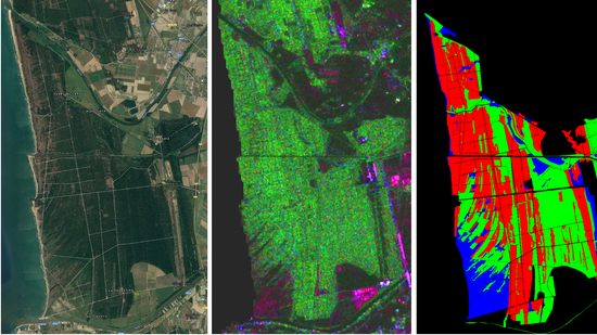
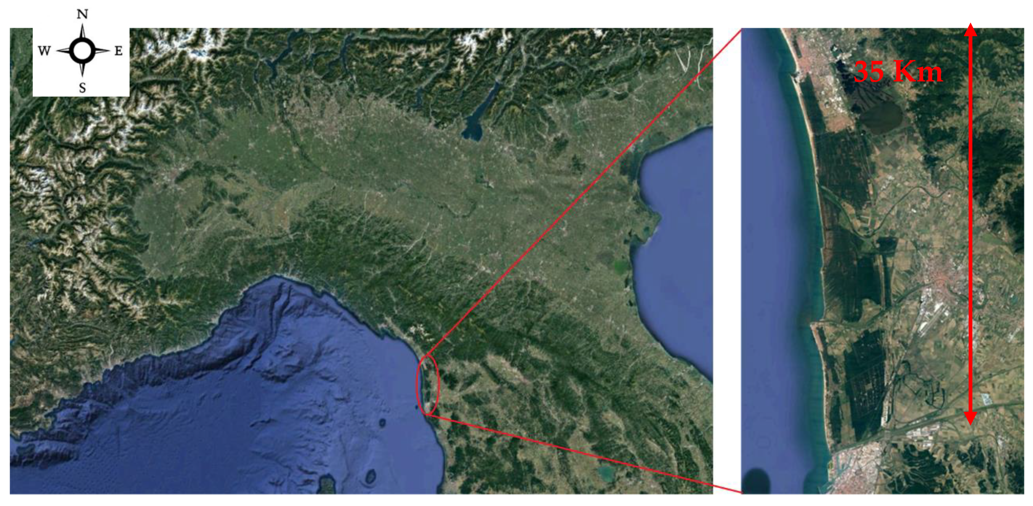
Figure 4b, an RGB visualization of ALOS/PALSAR images collected on San Rossore area in 7th June 2009 at three polarizations is shown (R: HH pol., G: HV pol. and B: VV pol.), which allows a preliminary but clear identification of forest areas with respect to other type of surfaces. In
Figure 4a, an optical Google Earth image is also shown for a visual match. Comparing both images, forest areas recognizable in the Google Earth image correspond to green pixels in the RGB composite, pointing out the importance of HV polarization in identification of forest areas. Indeed, cross polarization at the L-band was mainly sensitive to inclined cylinders of dimensions comparable to the carrier radar wavelength (about 20 cm) and therefore represented by thick branches and trunks. When inclined cylinders were observed, the backscattering coefficient shows a maximum whose position tended toward lower diameter values as the frequency increased [
10,
30]. For each frequency the range of diameters producing the maximum values of the backscatter coefficient was a fraction of the wavelength (1/10-1/20).
3.2. Temporal Average Backscatter Images
The image dataset for classification was built starting from all the available data reported in
Table 1, with the only exception of quad-pol PALSAR acquisition that had been excluded a-priori for sake of consistency with the other SAR data in terms of incidence angle and type of product. The co-registered image stack had been initially split in four sub-stacks, namely PALSAR HH, PALSAR HV, ASAR VV and CSK2 HH, grouping together the images sensed by the same sensor and the same polarization. The statistics of the backscattering coefficient evaluated over each sub-stack for coniferous and broadleaf forests are reported in
Table 2. The mean backscattering values were close (gap of about 0.5 dB) in PALSAR HH and PALSAR HV, whereas they increase for broadleaf with respect to coniferous (gap greater than 1.5 dB) in ASAR VV and CSK2 HH. Hence, the different sensitivities at various frequencies to forest characteristics were well pointed out. At X- and C-bands, the operative wavelength (between 3 and 6 cm, respectively) was comparable with the dimensions of needles and leaves, being more sensitive these surface characteristics. On the other hand, at L-band, the longer wavelength (about 20 cm) had a higher penetration power inside vegetation cover and was less influenced by crown characteristics. Furthermore, by considering the standard deviation of each sub-stack, it emerged that the horizontal polarization (PALSAR HH and CSK2 HH) exhibited the highest dispersion. Interestingly, if the median absolute deviation (M.A.D.) was used instead of the standard deviation, the contribution of speckle and outliers was reduced (up to –3.99 dB for the broadleaf class in PALSAR HH). Thus, a limited temporal dispersion of data for sensor-polarization pair was assumed.
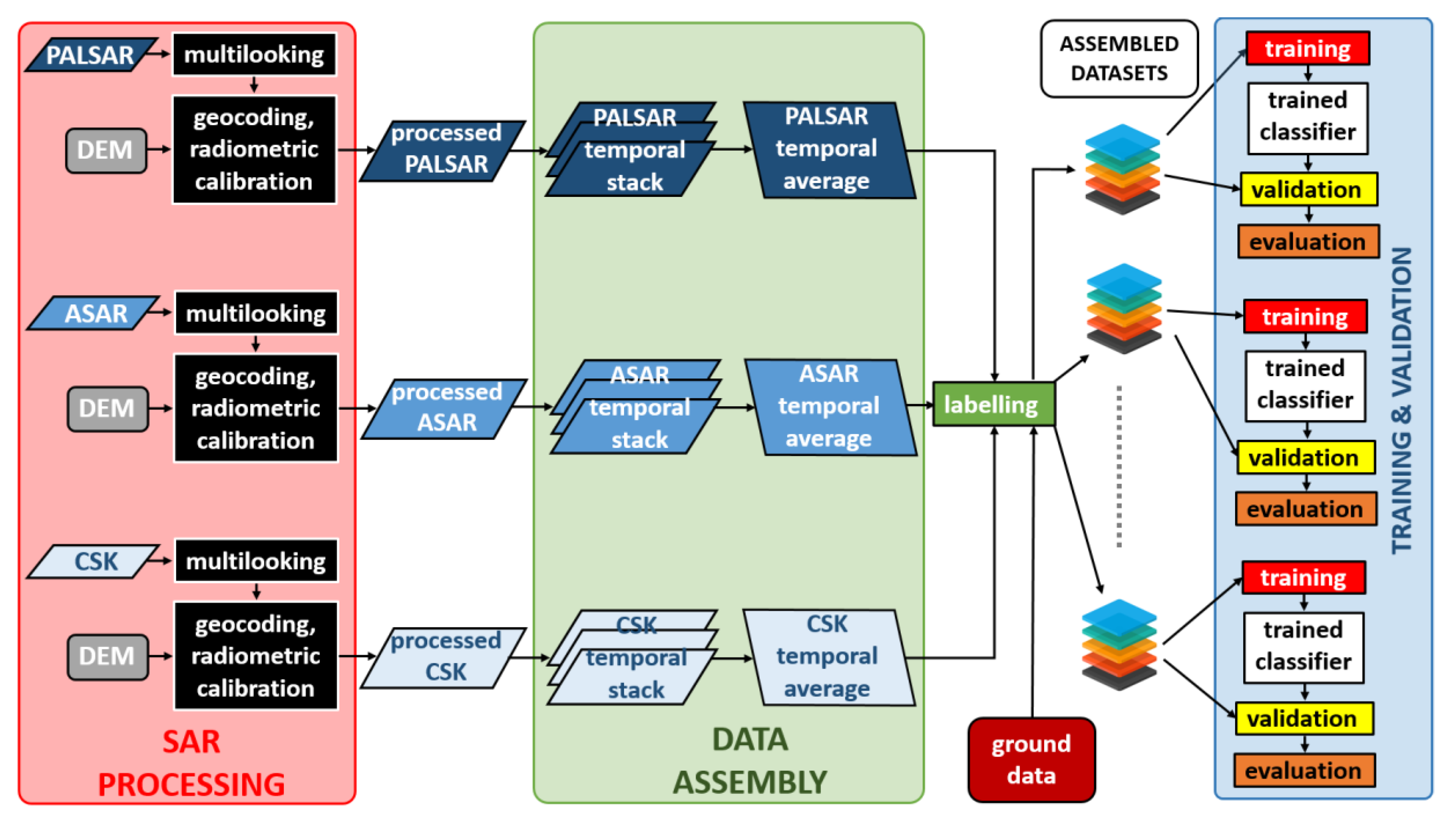
The images of each sub-stack were subsequently averaged, in order to obtain four temporal average backscatter coefficient images. This processing was motivated by two reasons: i) improve the signal intensity with respect to speckle noise and ii) minimize the seasonal effects (such as soil moisture variations, presence/absence of leaves, higher or lower tree water content) on the classification procedures. As to the effects of soil moisture, model simulations in [
31] pointed out that for high cover fraction, typical of the most of the plots of the San Rossore forest, the soil contribution becomes negligible at L-band for growing stock volume values higher than 50 m
3/ha.
Radiometric discrimination among classes was preserved in the temporal average backscattering coefficient images. This fact can be appreciated, for instance, by visual inspecting the PALSAR HH and PALSAR HV images, reported in
Figure 5a,b, respectively. Different forest features could be weakly identified in the former image; instead, they were visible in the latter, due to the presence of inclined cylinders represented by branches and trunks. However, also in this case, the discrimination between the two types of forest was not trivial. In
Figure 5c,d, ASAR VV and CSK2 HH images were respectively represented; in these images, the features inside the forest area were more evident than in the previous ones, and the temporal average backscatter coefficient seemed more suitable to discriminate coniferous and broadleaf forests.
The additional contribution of interferometric coherence [
32] for classification purposes was also investigated. Nevertheless, it was not reported in this work because no relevant improvement emerged in our test cases.
3.3. Classification Dataset
The classification dataset was obtained by stacking the temporal average backscattering coefficient images described in
Section 3.2. For convenience, the composition of the classification stack is listed in the following:
PALSAR HH stack, which is the temporal average of 11 HH polarized PALSAR images collected from single and dual polarization acquisitions;
PALSAR HV stack, which is the temporal average of 5 HV polarized PALSAR images collected from dual polarization acquisitions;
ASAR VV stack, which is the temporal average of 12 HV polarized ASAR images;
CSK2 HH stack, which is the temporal average of 7 HH polarized CSK2 images.
The classification of SAR images is generally impaired by speckle noise. Even though the multitemporal averaging intrinsically introduces a speckle reduction, a performance margin was empirically observed when applying a despeckling stage, especially for the smallest temporal stack (PALSAR HV). Thus, a 7 × 7 sliding window Kuan filter was applied to each image of the classification stack, as a tradeoff between speckle removal and reduced computational burden [
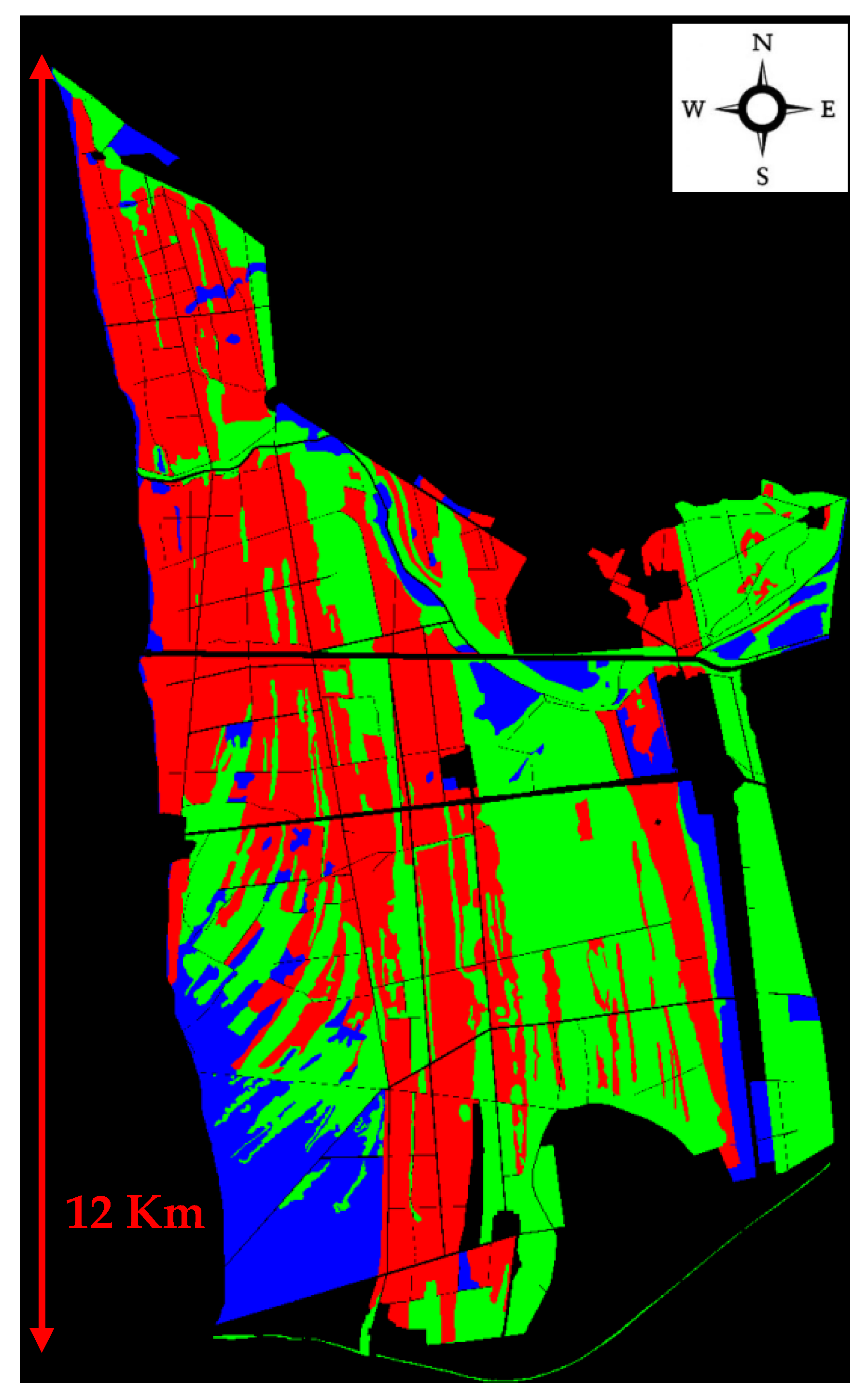
33]. After masking of unclassified and no-data-pixel, a total of 365,541 labeled samples were extracted. The prior distribution of the labeled samples is the following: coniferous (39.4%), broadleaf (41.3%) and non-forest (19.3%). Each sample is a four-element vector whose components were the temporal average backscattering coefficients evaluated at the same pixel in the classification stack. The sample label was the class (coniferous, broadleaf and non-forest) of the corresponding pixel according to the reference map (
Figure 2).
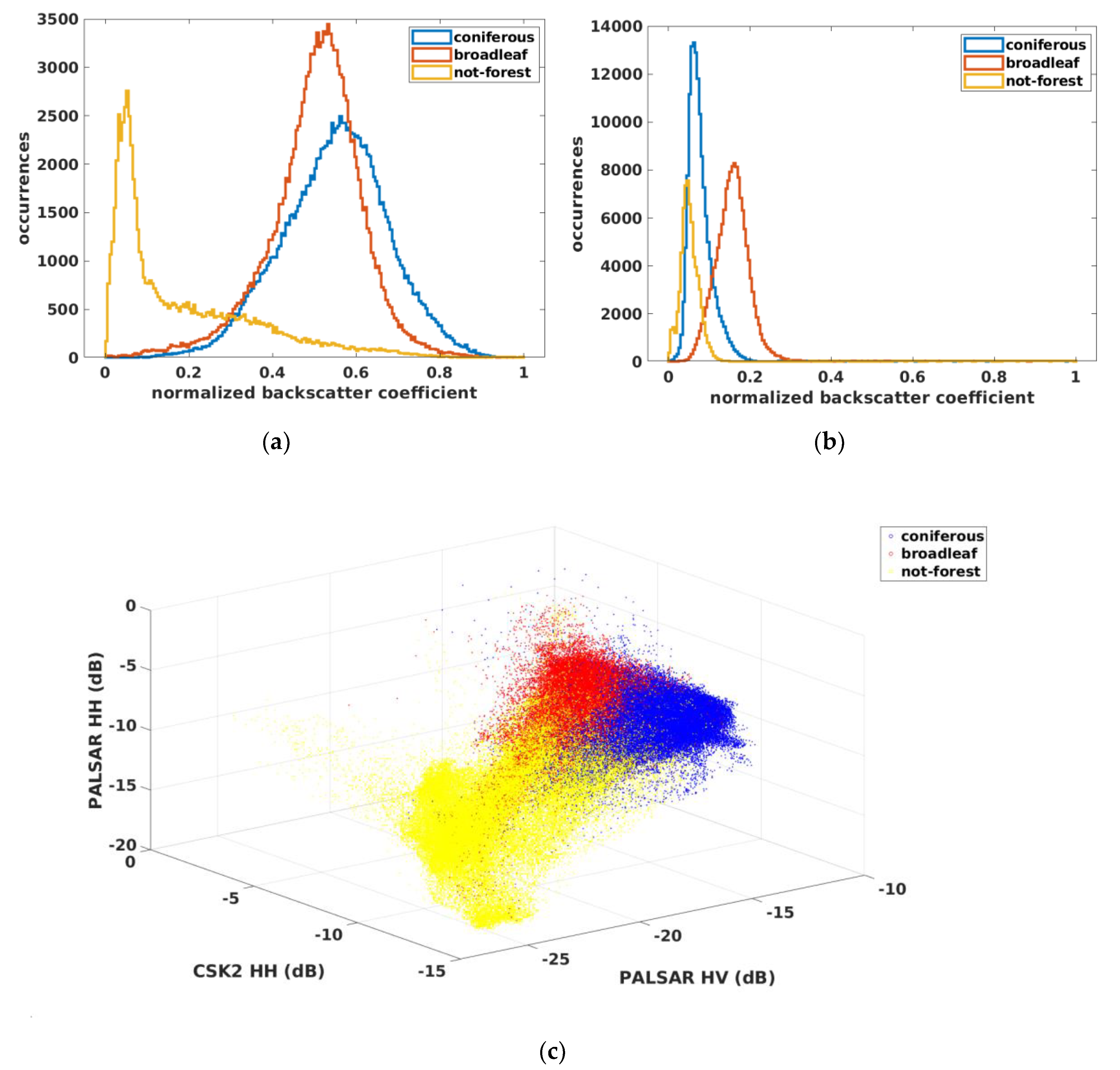
In
Figure 6, the distributions related to PALSAR HV and the CSK2 HH components collected in the classification dataset are shown. It can be observed that coniferous and broadleaf classes were distributed according to monomodal distributions with a high degree of symmetry. On the contrary, the non-forest class was remarkably asymmetric. This is explained by considering the heterogeneity of this class, where different surface features as marine environment, agricultural fields and small anthropic settlements are contained. By visual inspection, it can be noted that coniferous and broadleaf classes were better distinguished in the X-band (
Figure 6b), whereas non-forest was more separated in the C-band (
Figure 6a). The improvement in terms of separation among classes when using of three components, namely PALSAR HV, CSK2 HH and PALSAR HV, could be appreciated in
Figure 6c, where the joint three-dimensional distribution was reported. Thus, an improvement in the performance of classifiers is expected by using the bands jointly.
3.4. Image Classification Methods
The classification of the test site was carried out by using the following supervised classification methods belonging to the machine learning framework:
Random forest (RF);
AdaBoost with decision trees (AB);
K-nearest neighbors (kNN);
Feed forward artificial neural networks (FF-ANNs);
Support vector machines (SVM);
Quadratic discriminant (QD).
Random forest (RF) is a classification method belonging to the ensemble learning methods [
34]. Ensemble classifiers perform decisions by aggregating the classification results coming from several weak classifiers. In RF, the weak classifiers are decision trees [
35] and predictions are performed by the majority, i.e., the predicted class is the most voted by all the weak classifiers. Decision trees are trained by randomly drawing with replacement a subset of training data (bagging). The RF algorithm has been demonstrated to reduce both the bias and the overfitting with respect to decision trees, as well as making unnecessary the pruning phase [
36]. Two main parameters must be set in RF: the number of features in the random subset at each node and the number of decision trees [
37]. All these aspects, as well as a contained computation burden (compared, for instance, to SVM) and outperforming classification results, have contributed to make RF very popular in the study of land cover, too (see, for instance, [
36,
37,
38,
39,
40]).
Boosting algorithms generally refer to the method that combines weak classifiers to get a strong classifier [
41]. AdaBoost with decision trees (AB) [
42] is a boosting ensemble classification method whose prediction relies on a weighted mean of the outputs of several weaker decision trees (the higher the weight, the more reliable the decision tree). The iterative training algorithm selects a decision tree at each step, in order to minimize a cost function, and update the weights. This process has been shown to improve the overall performance under some optimality measure [
42]. AdaBoost has been already considered in the remote sensing literature, e.g., for tree detection [
43], land cover classification in tropical regions [
44] and land cover classification carried out on hyperspectral images [
45]. Nevertheless, the main drawbacks of AB are its sensitivity to outliers and the number of hyperparameters to be optimized in order to improve the classification performance.
The K-nearest neighbors (KNN) algorithm is another popular classification method [
46]. In KNN, the training dataset corresponds to a set of labeled points in the space of features. The prediction is performed by only considering the classes of the k training samples that are closest to test sample, according to a given metric. There are many strategies to perform this decision, e.g., majority vote, weighted distance [
47] or by using Dempster–Schafer theory [
48]. An integration of KNN and SVM has been also proposed [
49]. The basic KNN algorithm usually attains suboptimal classification performance compared to other more recent methods and can be memory intensive for a high number of features. Nevertheless, due its plain logic and configuration (the main parameter is the number of neighbor k), it has been thoroughly used as benchmark in the remote sensing community [
39,
50,
51].
An algorithm based on feed forward artificial neural networks (FF-ANNs) has been also considered for the comparison. FF-ANN is conceived for establishing non-linear relationships between inputs and outputs [
52] and therefore cannot be regarded as a classification algorithm strictly speaking. However, they can be applied to almost any kind of input–output relationships and their ability in solving non-linear problems has been largely proven [
53]. FF-ANN is composed of a given number of interconnected neurons, distributed in one or more hidden layers, that receive data, perform simple operations (usually additions and products) and propagate the results. The FF-ANN training is based on the back propagation (BP) learning rule, which is a gradient descendent algorithm aimed at minimizing iteratively the mean square error (MSE) between the network output and the target value. As a main disadvantage, FF-ANN is sensitive to outliers: a training representative of the testing conditions is therefore mandatory for obtaining satisfactory results [
54]. In this study, FF-ANN was adapted to act as classifiers by simply rounding the obtained outputs to the closest integer.
Another popular algorithm for classification is represented by support vector machine (SVM). In SVM, the space of features is divided in subspaces by means of hyperplanes, named decision planes, and the prediction is performed according to the subspace that the test point belongs to (see, for instance, [
55]). The decision planes are computed during the training phase searching for the maximum margin, according to some distance function. SVM have been also extended to deal with nonlinear separation hypersurfaces [
55,
56], allowing us to map the features in a higher-dimensional feature space through some nonlinear mapping and formulating a linear classification problem in that feature space by means of kernel functions. SVM-based methods are very common due to their good classification performance (see, for instance, [
24,
37,
39,
40,
50,
57]). As a drawback, SVM may require a fine tuning of many hyperparameters to obtain the optimal result. Furthermore, the training of SVM classifiers is performed by means of quadratic programming optimization routines [
55]; thus, the training time is usually higher than, for instance, RF.
The quadratic discriminant classifier (QD) pertains to the discriminant analysis framework [
58]. In QD, data samples are assumed to be generated according to a Gaussian mixture distribution. The mean and the covariance matrix of each component are estimated by using the training data set belonging to the corresponding class. The prediction is performed by computing the posterior probability that the test sample belongs to each class and selecting the class for which the maximum is attained. Despite of the simplistic statistical hypothesis, QD can often deal with complex data models, exhibiting a competitive classification performance [
59,
60]. Furthermore, the training and decision phases are usually extremely fast.

 ,
, 


