Intercomparison of Machine-Learning Methods for Estimating Surface Shortwave and Photosynthetically Active Radiation


Abstract
1. Introduction
2. Data
2.1. Remote Sensing
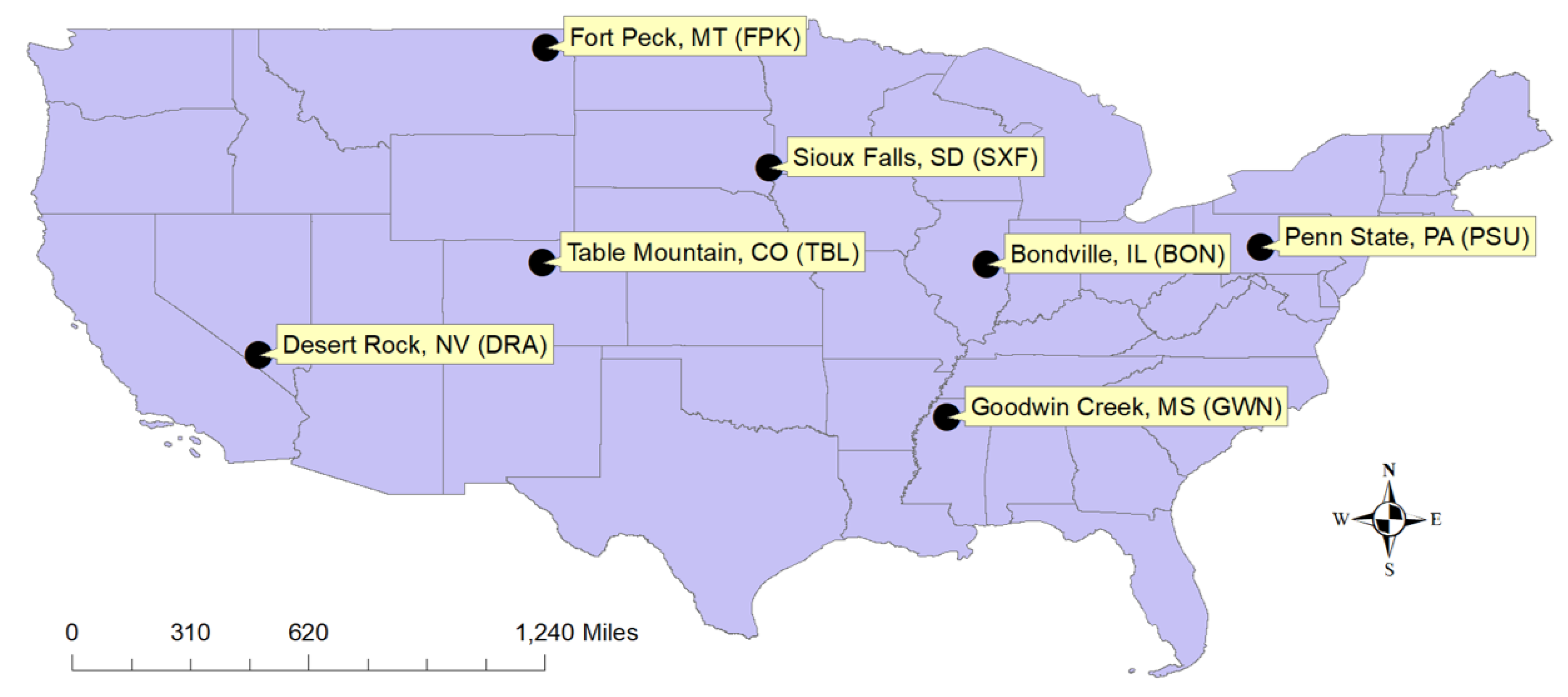
2.2. SURFRAD
2.3. Training and Validation Data Sets
3. Methods
3.1. Modeling SSR and PAR with Machine-Learning Methods
3.1.1. Linear Methods
3.1.2. Decision Tree Methods
3.1.3. Neural Networks
3.1.4. Kernel Methods
3.2. Data Filtering, Parameter Tuning, and Training
3.3. Cross Validation
4. Results
4.1. Model Performance
4.2. Time Series and Site Analysis
5. Discussion
6. Conclusions
Author Contributions
Acknowledgments
Conflicts of Interest
References
- Wild, M. Enlightening global dimming and brightening. Bull. Am. Meteorol. Soc. 2012, 93, 27–37. [Google Scholar] [CrossRef]
- Liang, S.; Wang, D.; He, T.; Yu, Y. Remote sensing of earth’s energy budget: Synthesis and review. Int. J. Digit. Earth 2019, 12, 737–780. [Google Scholar] [CrossRef]
- Wild, M.; Folini, D.; Schär, C.; Loeb, N.; Dutton, E.G.; König-Langlo, G. The global energy balance from a surface perspective. Clim. Dyn. 2013, 40, 3107–3134. [Google Scholar] [CrossRef]
- Streets, D.G.; Wu, Y.; Chin, M. Two-decadal aerosol trends as a likely explanation of the global dimming/brightening transition. Geophys. Res. Lett. 2006, 33. [Google Scholar] [CrossRef]
- Qian, Y.; Wang, W.; Leung, L.R.; Kaiser, D.P. Variability of solar radiation under cloud-free skies in China: The role of aerosols. Geophys. Res. Lett. 2007, 34. [Google Scholar] [CrossRef]
- Haywood, J.M.; Bellouin, N.; Jones, A.; Boucher, O.; Wild, M.; Shine, K.P. The roles of aerosol, water vapor and cloud in future global dimming/brightening. J. Geophys. Res. Atmos. 2011, 116. [Google Scholar] [CrossRef]
- Nemani, R.R.; Keeling, C.D.; Hashimoto, H.; Jolly, W.M.; Piper, S.C.; Tucker, C.J.; Myneni, R.B.; Running, S.W. Climate-driven increases in global terrestrial net primary production from 1982 to 1999. Science 2003, 300, 1560–1563. [Google Scholar] [CrossRef]
- Running, S.W.; Nemani, R.R.; Heinsch, F.A.; Zhao, M.; Reeves, M.; Hashimoto, H. A continuous satellite-derived measure of global terrestrial primary production. AIBS Bull. 2004, 54, 547–560. [Google Scholar] [CrossRef]
- Milesi, C.; Hashimoto, H.; Running, S.W.; Nemani, R.R. Climate variability, vegetation productivity and people at risk. Glob. Planet. Chang. 2005, 47, 221–231. [Google Scholar] [CrossRef]
- Alton, P.; Ellis, R.; Los, S.; North, P. Improved global simulations of gross primary product based on a separate and explicit treatment of diffuse and direct sunlight. J. Geophys. Res. Atmos. 2007, 112. [Google Scholar] [CrossRef]
- Mercado, L.; Bellouin, N.; Sitch, S.; Boucher, O.; Huntingford, C.; Wild, M.; Cox, P. Impact of Changes in Diffuse Radiation on the Global Land Carbon Sink, 1901–2100. In Proceedings of the EGU General Assembly Conference Abstracts, Vienna, Austria, 19–24 April 2009; Volume 11, p. 8273. [Google Scholar]
- Kanniah, K.D.; Beringer, J.; North, P.; Hutley, L. Control of atmospheric particles on diffuse radiation and terrestrial plant productivity: A review. Prog. Phys. Geogr. 2012, 36, 209–237. [Google Scholar] [CrossRef]
- Cheng, S.J.; Bohrer, G.; Steiner, A.L.; Hollinger, D.Y.; Suyker, A.; Phillips, R.P.; Nadelhoffer, K.J. Variations in the influence of diffuse light on gross primary productivity in temperate ecosystems. Agric. For. Meteorol. 2015, 201, 98–110. [Google Scholar] [CrossRef]
- Liang, S.; Zheng, T.; Liu, R.; Fang, H.; Tsay, S.C.; Running, S. Estimation of incident photosynthetically active radiation from Moderate Resolution Imaging Spectrometer data. J. Geophys. Res. Atmos. 2006, 111. [Google Scholar] [CrossRef]
- Zhang, Y.; He, T.; Liang, S.; Wang, D.; Yu, Y. Estimation of all-sky instantaneous surface incident shortwave radiation from Moderate Resolution Imaging Spectroradiometer data using optimization method. Remote Sens. Environ. 2018, 209, 468–479. [Google Scholar] [CrossRef]
- Wang, D.; Liang, S.; Zhang, Y.; Gao, X.; Brown, M.G.; Jia, A. A New Set of MODIS Land Products (MCD18): Downward Shortwave Radiation and Photosynthetically Active Radiation. Remote Sens. 2020, 12, 168. [Google Scholar] [CrossRef]
- Van Laake, P.E.; Sanchez-Azofeifa, G.A. Simplified atmospheric radiative transfer modelling for estimating incident PAR using MODIS atmosphere products. Remote Sens. Environ. 2004, 91, 98–113. [Google Scholar] [CrossRef]
- Zhang, X.; Liang, S.; Wild, M.; Jiang, B. Analysis of surface incident shortwave radiation from four satellite products. Remote Sens. Environ. 2015, 165, 186–202. [Google Scholar] [CrossRef]
- Katkovsky, L.; Martinov, A.; Siliuk, V.; Ivanov, D.; Kokhanovsky, A. Fast atmospheric correction method for hyperspectral data. Remote Sens. 2018, 10, 1698. [Google Scholar] [CrossRef]
- Camps-Valls, G.; Gómez-Chova, L.; Muñoz-Marí, J.; Vila-Francés, J.; Amorós-López, J.; Calpe-Maravilla, J. Retrieval of oceanic chlorophyll concentration with relevance vector machines. Remote Sens. Environ. 2006, 105, 23–33. [Google Scholar] [CrossRef]
- Lázaro-Gredilla, M.; Titsias, M.K. Variational Heteroscedastic Gaussian Process Regression. In Proceedings of the 28th International Conference on International Conference on Machine Learning (ICML), Bellevue, WA, USA, 28 June–2 July 2011; pp. 841–848. [Google Scholar]
- Lázaro-Gredilla, M.; Titsias, M.K.; Verrelst, J.; Camps-Valls, G. Retrieval of biophysical parameters with heteroscedastic Gaussian processes. IEEE Geosci. Remote Sens. Lett. 2014, 11, 838–842. [Google Scholar] [CrossRef]
- Bishop, C.M. Pattern Recognition and Machine Learning; Springer: New York, NY, USA, 2006. [Google Scholar]
- Claverie, M.; Ju, J.; Masek, J.G.; Dungan, J.L.; Vermote, E.F.; Roger, J.C.; Skakun, S.V.; Justice, C. The Harmonized Landsat and Sentinel-2 surface reflectance data set. Remote Sens. Environ. 2018, 219, 145–161. [Google Scholar] [CrossRef]
- Justice, C.O.; Román, M.O.; Csiszar, I.; Vermote, E.F.; Wolfe, R.E.; Hook, S.J.; Friedl, M.; Wang, Z.; Schaaf, C.B.; Miura, T.; et al. Land and cryosphere products from Suomi NPP VIIRS: Overview and status. J. Geophys. Res. Atmos. 2013, 118, 9753–9765. [Google Scholar] [CrossRef] [PubMed]
- Skakun, S.; Justice, C.O.; Vermote, E.; Roger, J.C. Transitioning from MODIS to VIIRS: An analysis of inter-consistency of NDVI data sets for agricultural monitoring. Int. J. Remote Sens. 2018, 39, 971–992. [Google Scholar] [CrossRef] [PubMed]
- MOD021KM MODIS/Terra Calibrated Radiances 5-Min L1B Swath 1 km. Available online: https://modaps.modaps.eosdis.nasa.gov/services/about/products/c6/MOD021KM.html (accessed on 1 June 2017).
- MYD021KM MODIS/Aquaa Calibrated Radiances 5-Min L1B Swath 1 km. Available online: https://modaps.modaps.eosdis.nasa.gov/services/about/products/c6/MYD021KM.html (accessed on 1 June 2017).
- Ackerman, S.; Frey, R. MODIS Atmosphere L2 Cloud Mask Product (35_L2); NASA MODIS Adaptive Processing System, NASA Goddard Space Flight Center: Greenbelt, MD, USA, 2015.
- MOD03 MODIS/Terra Geolocation Fields 5-Min L1A Swath 1 km. Available online: https://modaps.modaps.eosdis.nasa.gov/services/about/products/c6/MOD03.html (accessed on 1 June 2017).
- MYD03 MODIS/Aqua Geolocation Fields 5-Min L1A Swath 1 km. Available online: https://modaps.modaps.eosdis.nasa.gov/services/about/products/c6/MYD03.html (accessed on 1 June 2017).
- Augustine, J.A.; Hodges, G.B.; Cornwall, C.R.; Michalsky, J.J.; Medina, C.I. An update on SURFRAD—The GCOS surface radiation budget network for the continental United States. J. Atmos. Ocean. Technol. 2005, 22, 1460–1472. [Google Scholar] [CrossRef]
- WMO OSCAR. Observing Systems Capability Analysis and Review Tool (OSCAR); World Meteorological Organization: Geneva, Switzerland; Available online: https://www.wmo-sat.info/oscar/ (accessed on 1 December 2019).
- Carter, C.; Liang, S. Evaluation of ten machine learning methods for estimating terrestrial evapotranspiration from remote sensing. Int. J. Appl. Earth Obs. Geoinf. 2019, 78, 86–92. [Google Scholar] [CrossRef]
- Santosa, F.; Symes, W.W. Linear inversion of band-limited reflection seismograms. SIAM J. Sci. Stat. Comput. 1986, 7, 1307–1330. [Google Scholar] [CrossRef]
- Tibshirani, R. Regression shrinkage and selection via the lasso. J. R. Stat. Soc. Ser. B (Methodol.) 1996, 58, 267–288. [Google Scholar] [CrossRef]
- Zou, H.; Hastie, T. Regularization and variable selection via the elastic net. J. R. Stat. Soc. Ser. B Statist. Methodol. 2005, 67, 301–320. [Google Scholar] [CrossRef]
- Hastie, T.; Tibshirani, R.; Friedman, J. The Elements of Statistical Learning: Data Mining, Inference, and Prediction; Springer: Berlin, Germany, 2009. [Google Scholar]
- Breiman, L. Bagging predictors. Mach. Learn. 1996, 24, 123–140. [Google Scholar] [CrossRef]
- LeCun, Y.; Bengio, Y.; Hinton, G. Deep learning. Nature 2015, 521, 436–444. [Google Scholar] [CrossRef]
- Kussul, N.; Lavreniuk, M.; Skakun, S.; Shelestov, A. Deep learning classification of land cover and crop types using remote sensing data. IEEE Geosci. Remote Sens. Lett. 2017, 14, 778–782. [Google Scholar] [CrossRef]
- Campagnolo, M.L.; Montano, E.L. Estimation of effective resolution for daily MODIS gridded surface reflectance products. IEEE Trans. Geosci. Remote Sens. 2014, 52, 5622–5632. [Google Scholar] [CrossRef]
- Latinne, P.; Debeir, O.; Decaestecker, C. Limiting the number of trees in random forests. In International Workshop on Multiple Classifier Systems; Springer: Berlin/Heidelberg, Germany, 2001; pp. 178–187. [Google Scholar]
- Oshiro, T.; Perez, P.; Baranauskas, J. How Many Trees in a Random Forest? In Proceedings of the 8th International Conference Machine Learning and Data Mining in Pattern Recognition (MLDM 2012), Berlin, Germany, 13–20 July 2012; Volume 7376. [Google Scholar] [CrossRef]
- Perner, P. Machine Learning and Data Mining in Pattern Recognition. In Proceedings of the 8th International Conference (MLDM 2012), Berlin, Germany, 13–20 July 2012; Volume 7376. [Google Scholar] [CrossRef]
- Xu, J.; Li, C.; Shi, H.; He, Q.; Pan, L. Analysis on the impact of aerosol optical depth on surface solar radiation in the Shanghai megacity, China. Atmos. Chem. Phys. 2011, 11, 3281–3289. [Google Scholar] [CrossRef]
- Lefèvre, M.; Oumbe, A.; Blanc, P.; Espinar, B.; Gschwind, B.; Qu, Z.; Wald, L.; Homscheidt, M.S.; Hoyer-Klick, C.; Arola, A.; et al. McClear: A new model estimating downwelling solar radiation at ground level in clear-sky conditions. Atmos. Meas. Tech. 2013, 6, 2403–2418. [Google Scholar] [CrossRef]
- Xu, X.; Du, H.; Zhou, G.; Mao, F.; Li, P.; Fan, W.; Zhu, D. A method for daily global solar radiation estimation from two instantaneous values using MODIS atmospheric products. Energy 2016, 111, 117–125. [Google Scholar] [CrossRef]
- Zhang, X.; Liang, S.; Zhou, G.; Wu, H.; Zhao, X. Generating Global LAnd Surface Satellite incident shortwave radiation and photosynthetically active radiation products from multiple satellite data. Remote Sens. Environ. 2014, 152, 318–332. [Google Scholar] [CrossRef]
- Gui, S.; Liang, S.; Wang, K.; Li, L.; Zhang, X. Assessment of three satellite-estimated land surface downwelling shortwave irradiance data sets. IEEE Geosci. Remote Sens. Lett. 2010, 7, 776–780. [Google Scholar] [CrossRef]


| Data | Years Avail. | Spatial Res. | Temporal Res. | Citation |
|---|---|---|---|---|
| MOD/MYD021KM TOA Reflectance | 2002–current | 1 km at nadir | instantaneous 1–2-day revisit | [27,28] |
| MOD/MYD35 Cloud Mask | 2002–current | 1 km at nadir | instantaneous 1–2-day revisit | [29] |
| MOD/MYD03 Geolocation | 2002–current | 1 km at nadir | instantaneous 1–2-day revisit | [30,31] |
| SURFRAD | 2003–current | 10 m footprint | 3-min before 2005 1-min since 2005 | [32] |
| Method | SSR | SSR RMSE () | SSR Bias () | PAR | PAR RMSE () | PAR Bias () |
|---|---|---|---|---|---|---|
| RLR | 0.68 | 170 (29%) | −11 | 0.70 | 69 (29%) | −3 |
| LASSO | 0.68 | 170 (29%) | 28 | 0.70 | 70 (29%) | 11 |
| ELASTIC NET | 0.69 | 170 (29%) | 29 | 0.70 | 70 (29%) | 11 |
| DECISION TREE | 0.62 | 190 (31%) | −8 | 0.60 | 82 (31%) | −3 |
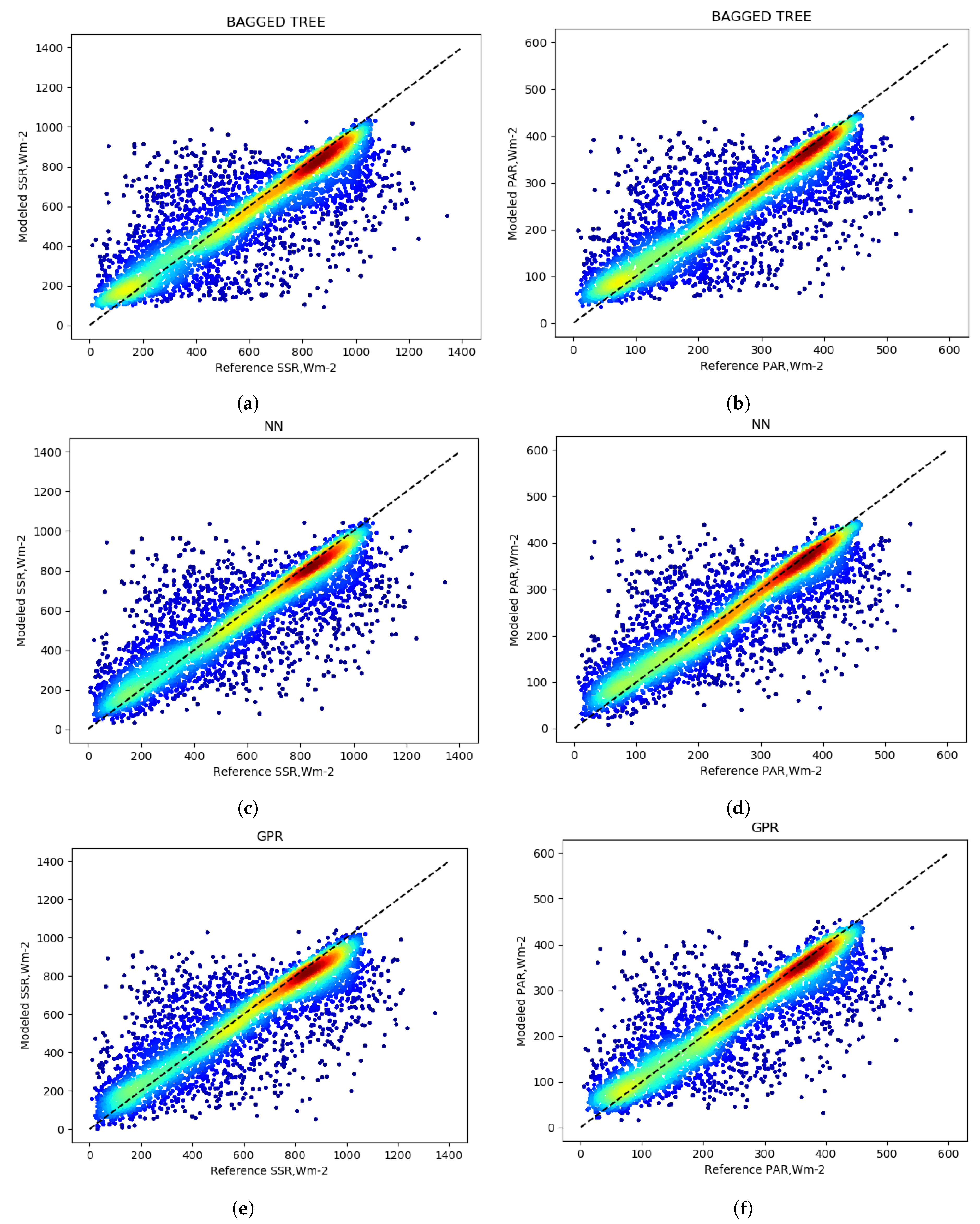
| BAGGED TREE | 0.77 | 144 (23%) | −8 | 0.76 | 61 (23%) | −2 |
| BOOSTED TREE | 0.73 | 155 (25%) | −11 | 0.73 | 65 (24%) | −3 |
| NN | 0.78 | 138 (22%) | −4 | 0.78 | 59 (22%) | −1 |
| KRR | 0.75 | 149 (24%) | −7 | 0.75 | 62 (23%) | −1 |
| GPR | 0.78 | 140 (23%) | −5 | 0.78 | 59 (22%) | −2 |
| Method | std | RMSE () | std () | Bias () | std () | |
|---|---|---|---|---|---|---|
| RLR | 0.62 | 0.08 | 183 (30%) | 25 | 5 | 9 |
| LASSO | 0.65 | 0.07 | 182 (30%) | 18 | 51 | 12 |
| ELASTIC NET | 0.65 | 0.07 | 182 (30%) | 19 | 50 | 10 |
| DECISION TREE | 0.60 | 0.01 | 193 (32%) | 4 | −2 | 7 |
| BAGGED TREE | 0.77 | 0.01 | 140 (23%) | 6 | 0 | 6 |
| BOOSTED TREE | 0.73 | 0.02 | 151 (25%) | 7 | 1 | 7 |
| NN | 0.78 | 0.02 | 136 (22%) | 7 | 1 | 6 |
| KRR | 0.76 | 0.02 | 141 (23%) | 7 | 0 | 5 |
| GPR | 0.78 | 0.02 | 138 (23%) | 7 | 0 | 5 |
| Method | std | RMSE () | std () | Bias () | std () | |
|---|---|---|---|---|---|---|
| RLR | 0.63 | 0.08 | 78 (30%) | 10 | 2 | 4 |
| LASSO | 0.65 | 0.06 | 77 (29%) | 8 | 22 | 5 |
| ELASTIC NET | 0.65 | 0.06 | 78 (29%) | 8 | 22 | 5 |
| DECISION TREE | 0.61 | 0.01 | 81 (31%) | 1 | −1 | 2 |
| BAGGED TREE | 0.77 | 0.02 | 60 (23%) | 2 | 0 | 2 |
| BOOSTED TREE | 0.73 | 0.02 | 64 (24%) | 3 | 0 | 2 |
| NN | 0.79 | 0.02 | 58 (22%) | 3 | 0 | 2 |
| KRR | 0.77 | 0.02 | 60 (23%) | 3 | 0 | 2 |
| GPR | 0.77 | 0.03 | 59 (22%) | 4 | −1 | 2 |
| Method | std | RMSE () | std () | Bias () | std () | |
|---|---|---|---|---|---|---|
| RLR | 0.60 | 0.09 | 182 (31%) | 33 | 7 | 17 |
| LASSO | 0.63 | 0.07 | 184 (31%) | 31 | 54 | 36 |
| ELASTIC NET | 0.63 | 0.07 | 183 (31%) | 31 | 52 | 36 |
| DECISION TREE | 0.51 | 0.10 | 214 (36%) | 27 | −19 | 55 |
| BAGGED TREE | 0.74 | 0.04 | 149 (25%) | 13 | −11 | 42 |
| BOOSTED TREE | 0.70 | 0.04 | 155 (26%) | 10 | −2 | 24 |
| NN | 0.76 | 0.04 | 139 (23%) | 12 | −8 | 30 |
| KRR | 0.73 | 0.04 | 146 (25%) | 15 | 8 | 13 |
| GPR | 0.75 | 0.04 | 141 (24%) | 15 | −2 | 15 |
| Method | std | RMSE () | std () | Bias () | std () | |
|---|---|---|---|---|---|---|
| RLR | 0.60 | 0.09 | 78 (31%) | 14 | 3 | 7 |
| LASSO | 0.63 | 0.07 | 78 (31%) | 12 | 21 | 16 |
| ELASTIC NET | 0.63 | 0.07 | 78 (30%) | 12 | 21 | 16 |
| DECISION TREE | 0.54 | 0.05 | 88 (34%) | 7 | −4 | 17 |
| BAGGED TREE | 0.74 | 0.04 | 64 (25%) | 5 | −5 | 18 |
| BOOSTED TREE | 0.71 | 0.04 | 67 (26%) | 4 | 0 | 16 |
| NN | 0.76 | 0.04 | 59 (23%) | 5 | −1 | 9 |
| KRR | 0.67 | 0.11 | 72 (28%) | 21 | −1 | 4 |
| GPR | 0.75 | 0.03 | 61 (24%) | 5 | 0 | 9 |
© 2020 by the authors. Licensee MDPI, Basel, Switzerland. This article is an open access article distributed under the terms and conditions of the Creative Commons Attribution (CC BY) license (http://creativecommons.org/licenses/by/4.0/).
Share and Cite
Brown, M.G.L.; Skakun, S.; He, T.; Liang, S. Intercomparison of Machine-Learning Methods for Estimating Surface Shortwave and Photosynthetically Active Radiation. Remote Sens. 2020, 12, 372. https://doi.org/10.3390/rs12030372
Brown MGL, Skakun S, He T, Liang S. Intercomparison of Machine-Learning Methods for Estimating Surface Shortwave and Photosynthetically Active Radiation. Remote Sensing. 2020; 12(3):372. https://doi.org/10.3390/rs12030372
Chicago/Turabian StyleBrown, Meredith G. L., Sergii Skakun, Tao He, and Shunlin Liang. 2020. "Intercomparison of Machine-Learning Methods for Estimating Surface Shortwave and Photosynthetically Active Radiation" Remote Sensing 12, no. 3: 372. https://doi.org/10.3390/rs12030372
APA StyleBrown, M. G. L., Skakun, S., He, T., & Liang, S. (2020). Intercomparison of Machine-Learning Methods for Estimating Surface Shortwave and Photosynthetically Active Radiation. Remote Sensing, 12(3), 372. https://doi.org/10.3390/rs12030372