Abstract
To study the uncertainties of a collapse susceptibility prediction (CSP) under the coupled conditions of different data-based models and different connection methods between collapses and environmental factors, An’yuan County in China with 108 collapses is used as the study case, and 11 environmental factors are acquired by data analysis of Landsat TM 8 and high-resolution aerial images, using a hydrological and topographical spatial analysis of Digital Elevation Modeling in ArcGIS 10.2 software. Accordingly, 20 coupled conditions are proposed for CSP with five different connection methods (Probability Statistics (PSs), Frequency Ratio (FR), Information Value (IV), Index of Entropy (IOE) and Weight of Evidence (WOE)) and four data-based models (Analytic Hierarchy Process (AHP), Multiple Linear Regression (MLR), C5.0 Decision Tree (C5.0 DT) and Random Forest (RF)). Finally, the CSP uncertainties are assessed using the area under receiver operation curve (AUC), mean value, standard deviation and significance test, respectively. Results show that: (1) the WOE-based models have the highest AUC accuracy, lowest mean values and average rank, and a relatively large standard deviation; the mean values and average rank of all the FR-, IV- and IOE-based models are relatively large with low standard deviations; meanwhile, the AUC accuracies of FR-, IV- and IOE-based models are consistent but higher than those of the PS-based model. Hence, the WOE exhibits a greater spatial correlation performance than the other four methods. (2) Among all the data-based models, the RF model has the highest AUC accuracy, lowest mean value and mean rank, and a relatively large standard deviation. The CSP performance of the RF model is followed by the C5.0 DT, MLR and AHP models, respectively. (3) Under the coupled conditions, the WOE-RF model has the highest AUC accuracy, a relatively low mean value and average rank, and a high standard deviation. The PS-AHP model is opposite to the WOE-RF model. (4) In addition, the coupled models show slightly better CSP performances than those of the single data-based models not considering connect methods. The CSP performance of the other models falls somewhere in between. It is concluded that the WOE-RF is the most appropriate coupled condition for CSP than the other models.
1. Introduction
Typical geological disasters such as collapse, landslide and debris flow are widely distributed all over the world, threatening a lot of human lives and property, and resulting in increasingly serious environmental problems [1]. The collapse is a geological phenomenon where the rock and soil mass on a steep slope suddenly breaks away from the parent body under the action of gravity [2,3,4]. Collapse susceptibility prediction (CSP) can efficiently reflect the spatial occurrence probability of collapses in a certain area. However, the uncertainties of CSP will lead to high risk project construction, seriously restricting the land use in the collapse prone area. Hence, how to effectively carry out the CSP has become one of the focuses of the collapse research [5].
Obtaining an accurate CSP is the preliminary work of collapse risk assessments. By analyzing the correlations between environmental factors and the history collapses inventory, a prediction model can be established to predict the possible spatial positions of future collapses [4,6]. The CSP consists of four steps: basic data acquisition, collapse-environmental factors connection method, model training and testing, and collapse susceptibility mapping (CSM) and CSP performance evaluation, etc. [2,7]. With the rapid development of spatial data acquisition technologies, the quality of the collapses inventory and environmental factors have been greatly improved [8]. Among these technologies, remote sensing (RS) is mainly applied for the acquisition of collapse-related environmental factors [9,10,11]. Meanwhile, CSP modeling is performed through the spatial analysis tools in the GIS software [12]. Furthermore, the types of collapse-related environmental factors in a specific study area can be determined by a review of related literature and the physical geography and geological conditions of the study area [8,10,13]. This study mainly focuses on the uncertainty characteristics of nonlinear connection methods of collapse-environmental factors, and the data-based models for CSP. Furthermore, these uncertainty characteristics are assessed by several statistic methods.
The nonlinear correlation analysis between collapses and basic environmental factors (no trigger factors) is considered as an important link between collapse susceptibility indexes (CSIs) and environment factors [14]. Then, these connection values will be directly used as the inputs of data-based models [15,16]. At present, many methods have been developed to construct correlation, mainly including weight of evidence (WOE) [17], information value (IV) [17], probability statistics (PSs) [18], Index of Entropy (IOE) [19] and frequency ratio (FR) [20] methods. However, there is almost no specific evidence and/or literature evaluation to determine an appropriate connection method. The calculation processes and results of nonlinear connection methods will bring great uncertainties to the data-based models for CSP. In general, a rough or less than ideal connection method will lead to information loss and further reduce the model’s CSP performance; on the contrary, a reasonable and excellent connection method can contribute to obtaining the optimal input variables of data-based models and improve the reliability of CSP results. Therefore, it is of great significance to explore the influence degree of different connection methods on CSP modeling [21].
Meanwhile, many scholars have carried out in-depth analysis on the data-based modeling for CSP on the Geographic Information System (GIS) platform [22,23]. According to the Bragagnolo et al. [24], the data-based models mainly include heuristic, mathematical statistics [25] and machine learning models [26]. Heuristic and mathematical statistical models are widely used [25,27,28], such as the deterministic factor model [29], discriminant analysis method [30], analytic hierarchy process (AHP) [31] and multiple linear regression [32]. Machine learning models mainly include logistic regressions [33,34], artificial neural networks [7,23,35,36,37,38], decision trees (DTs) [39,40,41], random forests [42], support vector machines [20,43], ensemble learning [44] and Bayesian algorithms [45,46,47,48]. Data-based models exhibit a more excellent prediction performance in nonlinear modeling of CSP in a large range with only an input–output sample than that of the heuristic and mathematical statistical models [31,49]. This is because the machine learning models [15,50,51,52] can effectively deal with the nonlinear relationship between collapses and environmental factors, determine model parameters automatically and connect inputs with CSIs named as output. However, there is no consensus on which type of model is the most suitable for CSP. Meanwhile, a slight improvement of the CSP performance may also have a significant impact on the division of the collapse susceptibility levels (CSLs) [53].
Overall, two remarkable uncertainty factors, namely the connection method and data-based model, are challenges greatly influencing CSP performance [54,55]. In most cases, a specific connection method and a certain data-based model may have been used without providing any argument and assessment—the uncertainties of CSP are rarely discussed in depth [56]. In fact, the CSP effect and feasibility can be further understood through uncertainty analysis of the CSP results under the coupled conditions of different connection methods and different data-based models [57].
In summary, the uncertainties of the connection methods and data-based models used in CSP modeling are explored. The An’yuan County in China is used as the study area, five kinds of nonlinear connection method (probability statistics (PSs), frequency ratio (FR), information value (IV), index of entropy (IOE) and weight of evidence (WOE)), coupled with four types of data-based models (heuristic model with analytic hierarchy process (AHP), conventional mathematical statistics model with multiple linear regression (MLR) and machine learning model with C5.0 decision tree (C5.0) and random forest (RF)) to form 20 types of different conditions for CSP. Finally, the uncertainty features of the CSIs under each coupled condition are assessed using several methods, including the accuracy evaluation, the difference significance analysis and the distribution rules of CSIs.
2. Materials
2.1. Introduction of An’yuan County
An’yuan County is located in the lower reaches of the Ganjiang River in Jiangxi Province, China, with a longitude of 115°9′52″ E–115°37′13″ E and a latitude of 24°52′18″ N–25°36′52″ N. The approximately 2374.59 km2 study area is characterized by hills and mountainous topography, with elevations of 180–1150 m. This district has a subtropical monsoon climate with an average temperature of 18.7 °C and an average rainfall of 1640 mm/year. The lithology is dominated by magmatic rocks, followed by metamorphic rocks and clastic rocks, and carbonate rocks are the least distributed. In this area, collapses are triggered by plum rains, stream erosion, engineering geological activities, or combination triggers [58]. Plum rains result from the fact that, during June each year, cold air from the north meets warm air from the south, creating a rainy season. Most of the collapses occurred in the slope residual material and the Quaternary sediments.
2.2. Collapse Inventory and Environmental Factors
According to the collapse inventory data provided by the An’yuan Land Resources Bureau of Jiangxi Province, as of 2014, a total of 108 collapses had occurred in the study area (Figure 1). The position, areas and boundary information of these recorded collapses are mapped out by the Global Position System technology in the field survey process. These collapses are dominated by moderate and small collapses over an average area of 6000 m2 (Figure 2c). From the perspective of space, the distribution of collapses is mainly affected by the topographical features, types of rock and soil mass, distance to rivers and land cover types, etc. From the collapse evolution characteristics in An’yuan County and the related literature, 11 environmental factors were acquired and chosen from the data sources based on a geological map, remote sensing image and GIS platform, and the main data sources are listed in Table 1 [59]. Both the collapse inventory and the environmental factors were mapped with 30 m resolution grid units. Examples of collapses in the An’yuan County are shown in Figure 2.

Figure 1.
Geographical location of collapses: China (a), Jiangxi Province (b), An’yuan County (c).
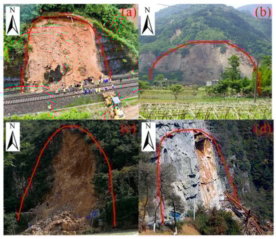
Figure 2.
Photos of typical collapses in the study area: soil collapse (a), soil collapse (b), mixture collapse of soil and rocks (c), rock collapse (d).

Table 1.
Data sources for collapse susceptibility prediction.
In this study, the environmental factors used for CSP are classified as follows: (1) topographic and geomorphic factors, including digital elevation model (DEM), slope, aspect, profile curvature, plane curvature and topographic relief; (2) land cover factors consist of the normalized differential vegetation index (NDVI) and normalized difference built-up index (NDBI); (3) hydrological factors with distance to rivers and modified normalized difference water index (MNDWI); (4) geological factors with lithology; lithology is the material basis of collapse development, which affects the permeability of rock and soil and shear strength of the slope. The lithology of the study area is magmatic rock, metamorphic rock, clastic rock and carbonate. The collapse-related environmental factors are acquired through RS and the GIS platform. The RS data include the DEM, Landsat TM 8 image and high-resolution images, and the GIS spatial analysis was performed in the ArcGIS 10.2 software.
2.2.1. Acquisition of Topographic and Hydrological Factors
The topographic and geomorphic factors for CSP were calculated and mapped through the three-dimensional analysis tool and data management tool in ArcGIS 10.2 software [40,60]. DEM is an important environmental factor for collapse evolution and a data source for other topographic elements. The whole study area ranges from 180 to 1151 m and was divided into 8 categories with equal intervals of 180–288 m, 288–368 m, 368–450 m, 450–540 m, 540–630 m, 630–733 m, 733–870 m and 870–1151 m. DEM can only reflect the changes of elevation values in larger regions, but it cannot reflect the ups and downs of terrain in smaller regions. To solve this problem, topographic relief is introduced to measure the relative changes of elevation values in smaller regions. The topographic relief was calculated through the statistical test and the maximum height difference method in a certain area in the ArcGIS 10.2 software. Slope has a direct relationship with the occurrence of collapse [61]. Only when the slope is attached to the slope can collapse occur, and the probability of collapse is different with different slopes. In this study, the slope angle values were reclassified into 8 categories with equal intervals of 0°–4°, 4°–8°, 8°–12°, 12°–16°, 16°–20°, 16°–24°, 24°–30° and 30°–90°. Aspect determines the scale of collapse formation under external factors such as rainfall, solar radiation and vegetation cover. Hence, the effects of aspect on collapse occurrence should not be neglected. Ultimately, nine groups of aspect are identified in this study area. Profile curvature and plan curvature are also extracted from DEM data. They affect the rate of collapse and weathering degree of rock mass on the slope. In this paper, profile curvature and plan curvature are divided into eight categories.
In addition, the river networks of An’yuan County are extracted by the hydrological analysis toolbox made up of fill, flow direction and flow accumulation tools, to reflect the effects of hydrological factors on landslide occurrences [62,63,64]. In the first step, the depressurization treatment of the DEM data with 30 m resolution was performed by the fill tool. In the second step, the flow direction tool was applied to determine the water flow direction of the filled DEM. In the third step, the flow accumulation tool was applied to determine the flow accumulation based on the water flow direction and DEM data. Finally, the river networks of the study area could be calculated and mapped by determining the flow accumulation of all grid units above a certain threshold.
2.2.2. Acquisition of NDVI, NDBI and MNDWI Factors
The NDVI, NDBI and MNDWI factors have important influences on the probability of landslide occurrence though affecting the shear strength of slope soils and controlling the surface and underground water migrations of the slope body [10,65,66]. These three significant remote sensing indexes were extracted from the above Landsat TM 8 image. The NDVI can be used to reflect the regional vegetation growth and coverage ratios (Equation (1)). The NDBI can be used to show the percentage of buildings on the ground surface of the study area (Equation (2)). Additionally, the MNDWI can reflect the surface hydrology and soil moisture information (Equation (3)). In these equations, the P (Red), P (NIR), P (Green) and P (MIR) are the measurements of the visible red band, near infrared band, green band and middle infrared band in the above Landsat 8 TM image, respectively.
3. Methodologies
3.1. Uncertainties of CSP: Connection Methods and Data-Based Models
The CSP accuracy is significantly dependent on the quality of input variables; therefore, it is important to select the collection methods of collapses inventory and environmental factors to obtain the input variables. In addition, the coupled models between collection methods and data-based models can also create many uncertainties. By analyzing the performance rules and influence degrees of the above two kinds of uncertainty factors on the prediction of CSIs, the influences of these uncertainty factors can be better reduced. For example, the literature shows that some researchers have recently used WOE or FR for collapse susceptibility modeling without any proper explanations [2,56]. In this study, based on the five nonlinear connection methods of PSs, FR, IV, IOE and WOE, the AHP, MLR, C5.0 and RF models were selected to establish 20 kinds of different coupled models for the CSP. The specific research steps are as follows (Figure 3):
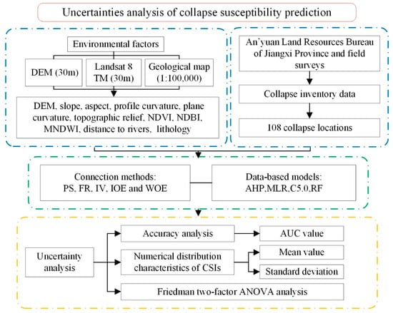
Figure 3.
The flowchart used in this research.
- (1)
- The data sources of collapse inventory and related environmental factors in the study area were obtained to construct the spatial datasets for CSP modeling;
- (2)
- A total of 20 different modeling conditions are proposed for CSP on the basis of the above five different connection methods and four different kinds of data-based models;
- (3)
- In the modeling processes, the CSP model was utilized, the CSM was drawn and the uncertainty analysis of the CSI was carried out under each coupled model condition;
- (4)
- The area under the ROC curve (AUC) [67] was used to evaluate the accuracy of the CSP results;
- (5)
- At the significance level of 0.05, the Friedman two-factor ANOVA analysis and test method were used to analyze the difference significance of the CSI distribution under each coupled model condition;
- (6)
- Numerical distribution characteristics of CSIs predicted by five correlation methods and four data-based models were analyzed from the perspective of mean values and standard deviation;
- (7)
- The optimal correlation method and data-based model coupled model condition was obtained through comparison analysis, so as to provide theoretical guidance for the CSP.
3.2. Collapse-Environmental Factors Connection Method
3.2.1. Probability Statistics
In general, the PSs method can be defined as the ratio of the area where collapses have occurred to the total collapse area for a given attribute interval of an environmental factor [18]. A greater value of means a higher correlation between the collapse and the related factor. The formula for calculating the collapse area ratio of each second-order factor is shown in Equation (4)— is the historical collapse area in the th state of the th environmental factor, and is the number of states under the th class factor.
3.2.2. Frequency Ratio
The FR method can be defined as the ratio of the area where collapses occurred in the total study area for a given attribute of an environmental factor, as show in Equation (5). is the number of collapse grid units that occurred in the attribute interval of an environmental factor; is the total number of collapse grid units in the study area; is the number of grid units of the attribute interval in an environment factor; represents the total number of grids in the study area. reveals the relative influence degree of each attribute interval of an environmental factor on the collapse occurrence [68]. A value greater than 1 indicates a higher correlation between collapse and environmental factors, otherwise the opposite is true.
3.2.3. Information Value
The collapse disasters are affected by multifactors. Under different geological environments, the degree and nature of the environmental factors that contribute to the collapse are different. The IV method was used to express the optimal combination of environmental factors under a certain geological environment, including the number and basic state of the environmental factors [31]. For a specific grid unit, the IV was used to consider the quantity and quality of all information acquired in a given area related to the collapse. In the specific calculation process, the total probability was usually estimated by using sample frequency for the calculation convenience. Hence, the formula of can be converted into Equation (6).
where is the information value of collapse occurrence when the environmental factor is in the state of , expresses the number of collapse grid units in the attribute interval of an environmental factor, is the total number of collapse grid units in the study area, denotes the number of grid units in the attribute interval of an environment factor and denotes the total number of grid units in the study area. When the value of is positive, the environmental factor in state j can provide the information of collapse occurrence. The greater the value of , the higher the probability of collapse occurrence. Otherwise, the opposite is true. In addition, when the value of is 0 or close to 0, the environmental factor has almost no contribution to the collapse occurrence and can be removed from the CSP modeling processes.
3.2.4. Index of Entropy
The IOE method was used to represent the degree of uncertainty of an environmental factor [69]. In the prediction of collapse susceptibility, IOE was used to express the influence degree of different environmental factors on the evolution of collapse disasters. Firstly, the probability density was calculated based on the frequency ratio analysis, as show in Equation (7). is the FR value of each environmental factor, denotes the number of categories and and represent the serial number and the class of the environmental factor, respectively.
Secondly, the probability density was substituted into Equation (8) to obtain the entropy value of each parameter; the information coefficient was calculated as Equation (9).
Finally, by coupling the information coefficient with the collapse occurrence probability, the final weight value of the parameter was calculated.
3.2.5. Weight of Evidence
The WOE is a quantitative method to predict the probability of an event based on Bayes’ theorem. For the collapse prediction, the spatial correlation between collapse and environmental factors was analyzed to obtain the distribution of various environmental factors at the collapse point. A pair of weights, and , for any environment factor was calculated:
where and are the weight values of the existence and nonexistence region of environmental factors, respectively; and are the number of the collapse grid units present on the existent and nonexistent regions of environmental factors, respectively; and are the number of the noncollapse units present on the existent and nonexistent regions of environmental factors, respectively. The difference between these weights , known as the relative coefficient, , represents a useful measure of the correlation between the evidence layer and the collapse events. For a positive correlation, the value of is positive, whereas for a negative correlation the value is negative; a weight of 0 is irrelevant. When data were missing, the weight was also considered to be 0.
3.3. Data-Based Models
3.3.1. Analytic Hierarchy Process
The AHP, a kind of decision-making method combining qualitative and quantitative analyses, was mainly used to quantify and model the selected environmental factors [70]. The AHP was established based on the internal dominant relationship among various environmental factors. Then, the weight values (ranging between 1 and 9) of environmental factors were determined by comparing environmental factors. The consistency ratio was defined based on Equation (13) to check the consistent features of the comparison matrix composed of these weight values.
where denotes the index of consistency obtained through Equation (14), suggests the random index for the comparison matrix , is the order in matric , denotes the eigenvector corresponding to the maximum eigenvalue of the matrix and denotes the th environmental factor. When the value of is less than 0.1, the comparison matric is satisfactory and consistent. Then, CSIs were calculated as Equation (15), where indicates the weight of the environmental factor :
3.3.2. Multiple Linear Regression
The MLR is often used to explore the correlations between multiple dependent variables and an independent variable. The value of the dependent variable was defined as Equation (16), where denotes the independent variable, denotes the regression coefficient and represents the error. The maximum likelihood value of parameters was calculated based on the least square method; then, necessary statistical tests were carried out to judge the goodness of fit of the model. The higher the value of is, the better the fitting degree is.
3.3.3. C5.0 Decision Tree
C5.0 uses the boosting method to improve the implementation efficiency and classification accuracy of the decision tree algorithm [71,72]. The C5.0 model can be constructed as four main steps [73]: (i) selecting the nodes of the optimal root segmentation tree using the training dataset and threshold with the highest gain ratio; (ii) finding the child nodes from two branch nodes produced by the tree structure; (iii) creating additional tree nodes that grow further with certain mathematical criteria, and in this process, children nodes that do not contribute to the model are eliminated; (iv) this process is continuous and repeated until all instances in the training dataset are assigned gain ratio values for leaf nodes or no remaining variables can be divided. After the initial decision tree was established, the model was verified by the testing dataset.
In summary, C5.0 construction consists of tree splitting, growth, pruning of child nodes, growth promotion and model closure. Compared with other artificial neural networks, this model is easier to be understood because it can clearly explain the processes of tree growth and removal [74].
3.3.4. Random Forest
The RF model is an integrated classification model composed of multiple classification trees and regression trees. The bagging technique (Bootstrap aggregation) was used to randomly select samples from the training dataset for classification and regression tree construction. Then, the optimal classification results were selected in the random subset of environmental factors with a given feature. The error of the model was evaluated by using a bag sample. The random forest integrates the results of all classification and regression trees, effectively avoiding the discontinuity of the predictive value of the decision tree and the sensitivity to the training dataset, so as to make the predictive value smoother, to prevent the overfitting of the model and to increase its stability [75].
3.4. Uncertainty Analysis of Results
3.4.1. ROC Curves and AUC Analysis
The ROC was used to evaluate the overall performance of the prediction model based on the quantitative indicators [76,77]. The ROC curve was calculated as follows: First, the values of CSIs were calculated, and various collapse samples in the testing dataset were sorted. Then, different truncation points were selected in this order. Next, whether each landslide sample was positive was determined. Finally, the “true positive rate” and “false positive rate” of the current classifier were calculated each time as the vertical and horizontal axis of the ROC curve [78]. To further quantify the classification performance of different models, the AUC (Area under ROC) was used as the specific evaluation index.
3.4.2. Statistical Law Analysis of CSI
The mean value and standard deviation (SD) were used to reflect the average level and dispersion degree of the CSIs distribution, respectively, and further to reveal the classification effects of different data-based models. The mean value and SD were adopted to reveal the predictive performance of the collapse susceptibility modeling under the coupled conditions of the connection method and the data-based model by analyzing the numerical distribution characteristics of the CSIs on the whole. By comparison and analysis, the optimal coupled condition could be obtained. The mean value and SD have a certain objectivity and provide theoretical guidance for the study of CSP.
Friedman two-factor ANOVA analysis and test by rank method were used to compare the significant differences between different CSP models. The Friedman test was used to test for significant differences between a set of models; the null hypothesis states the equality between the median values of two groups. Hence, if the probability of a hypothesis at the significant level of α = 0.05 (or 5%) was true, then the null hypothesis was rejected and vice versa [79]. To assess the significant differences between two models, the signed-rank test was used. Based on this test, the performances of these models were ranked. The higher the average rank is, the better the model performance is. The significance difference level and average rank were used to further analyze the uncertainties of connection method and data-based model to obtain the CSP model with a high reliability and accuracy.
4. Results
4.1. Collapse-Related Environmental Factor and Connection Results
The collapse inventory and environmental factors in the study area were obtained as shown in Table 2, through in-depth analysis of various factors affecting the evolution of collapses. The data types of continuous environmental factors were divided into eight attribute levels using the natural break point method [80,81], and the aspect of the flat ground was separately divided into one class and set to −1, while discrete types such as lithology and distance to rivers were classified into four classes.
Table 2.
Environment factors and calculation results of all connection methods.
(1) Relationships between collapses and topography.
The study area is located in the mountain boundary zone, mainly composed of low mountains and hills, with large topographic relief [82,83]. The elevation, slope, aspect, plane curvature, profile curvature and topographic relief were extracted from DEM as topographic and geomorphic factors, as shown in Figure 4. Taking slope as an example, the slopes in the study area were divided into eight attribute intervals, as shown in Figure 4b. The PSs regarding the occurrence of collapses were normally distributed when slopes ranged from 0° to 58.3° with a peak value of 16°. The FR values greater than 1 in the slope were greater than 16°, which is connected with the frequency of spatial classification, showing the strong spatial correlations between occurrence of collapses and the slope (Figure 5).
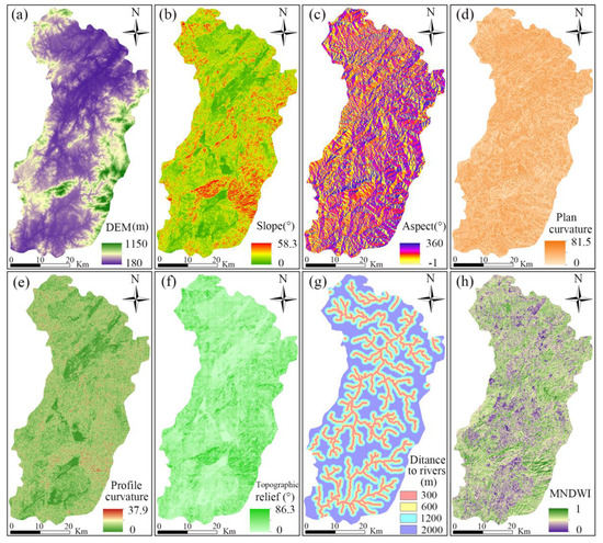
Figure 4.
Topographical factors: (a) Digital Elevation Model (DEM), (b) Slope, (c) Aspect, (d) Plan curvature, (e) Profile curvature, (f) Topographic relief, (g) Distance to rivers and (h) modified normalized difference water index (MNDWI).

Figure 5.
Effects of slope on collapse occurrence.
More specifically, according to the statistics in Table 2, within the slope range of 16°–20°, the values of PS and FR are 0.3 and 1.7, respectively; the IV and WOE show strong and positive correlations with collapse occurrence; the IOE shows that the weight of slope is 0.1458, second only to lithology. The results of these connection method suggest that, the slope has a very important role on the collapse occurrence, and further suggest that all the connection methods can reflect the effect of environmental factors on collapse susceptibility on the whole [84].
(2) Relationships between collapse and hydrological factors.
The collapse is largely affected by the distance to the river and the stream. Due to the erosion of the river, the stability of the slope rock and soil mass deteriorates with the increase in soil moisture content [85,86]. According to statistical calculation, the area with a distance of less than 300 m to the river system has the highest concentration of collapses (35%). MNDWI is commonly used to reflect water information at the surface; the value of MNDWI in the region ranges from 0 to 1, and most of the collapses occur between 0.392 and 0.498 with the maximum FR (1.214) (Table 2). The distance to the river and MNDWI (Figure 4g,h) were used to characterize the influence of hydrological environment on collapse evolution [87,88].
(3) Relationships between collapse and land cover factors.
The NDBI and NDVI were selected as land cover factors to reflect the influence of building distribution and natural vegetation on collapse evolution (Figure 6a,b). It can be seen from Table 2, when the NDBI values range between 0.49 and 0.6, that the calculation results of these collection methods of PS, FR, IV and WOE are all at their maximum values, which are 0.2515, 1.4969, 0.1752 and 0.7543, respectively. NDVI was used to quantitatively estimate vegetation growth and coverage. When the NDVI is smaller than 0.39, the area is prone to collapse occurrence.
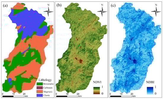
Figure 6.
Land cover, hydrology and geological factors: (a) Lithology, (b) normalized differential vegetation index (NDVI) and (c) normalized difference built-up index (NDBI).
(4) Relationships between collapse and lithology.
The lithology of An’yuan County is reflected by the types of rock and soil in this study. The types of rock and soil represent the material basis of collapse and greatly affect the collapse evolution. The values of PS and FR under the metamorphic rock are, respectively, up to 0.4388 and 1.3636, and those under the clastic rock are, respectively, 0.3356 and 1.2971. In addition, under the condition of both metamorphic and clastic rock types, the connection methods of IV and WOE have positive correlations with collapse occurrence, and the IOE suggests that the factor of lithology has the highest weight value of 0.2058 (Table 2). The other types of rock and soil are less distributed in this region. In short, the occurrence of collapse is relatively high in the areas with metamorphic and clastic rock types, and is relatively low in the areas with magmatic rock. In addition, very few carbonate rocks are distributed in this region, and as a result, the rule of collapse occurrence in this region is not clear.
4.2. Preparation of Spatial Dataset
The whole study area was divided into 2,655,972 grid units under the grid resolution of 30 m × 30 m. All of the 11 environment factors were reassigned by the calculation results of the five collection methods, then these reassigned environment factors were used as input variables of CSP models. At the same time, a total of 108 recorded collapse polygons were divided into 1463 collapse grid units, which were assigned to 1, while the same number of randomly selected noncollapse grid units were assigned to 0. These collapse and noncollapse grid units were randomly divided into model training sets and testing sets by a proportion of 70%/30%. Finally, all the grid units with connection values in the study area were put into the four models, respectively, to calculate the CSIs, which were divided into five levels: very high (10%), high (20%), m rate (20%), low (20%) and very low (30%).
4.3. Results of CSP Modeling in An’yuan County
4.3.1. CSP Using Heuristic Model: Analytic Hierarchy Process
Based on the calculation of the judgment matrix, the relevant parameters of the AHP model are: CI of 0.1055, RI of 1.54 and CR of 0.068, indicating that the provided pairwise comparison matrix has a reasonable level of consistency. Hence, the calculated weights of the environmental factors are reliable. The final weights of the 11 environmental factors obtained after normalization treatment are as follows: DEM (0.1101), slope (0.2504), aspect (0.0592), profile curvature (0.0413), surface curvature (0.0924), topographic relief (0.0504), lithology (0.1412), distance to the rivers (0.0896), NDVI (0.0521), NDBI (0.0693) and MNDWI (0.0481). The results show that slope and lithology contribute the most to the collapse evolution in the study area. The weight values of environmental factors and model input variables are imported into Equation (15) to calculate the CSIs of the study area. The model input variables obtained under different connect methods are different from each other, which results in the difference of the CSIs calculated by the AHP model.
4.3.2. CSP Using Conventional Mathematical Statistics Model: Multiple Linear Regression
The connection values of the 11 environmental factors calculated by the five connection methods were normalized and then taken as inputs to the MLR model. The collinearity diagnosis and significance test in the MLR were carried out to determine the suitable inputs. The results show that the variance inflation factor (VIF) of the 11 selected environmental factors was all less than 3, with a weak correlation and a significance of less than 0.05. All the environmental factors were statistically significant [89]. MLR modeling was carried out for collapse and noncollapse samples, and the regression coefficient of each environmental factor and the goodness of fit of the MLR model were calculated under five connection methods. The larger the regression coefficient is, the higher the contribution of the corresponding environmental factors to collapse development is. The greater the goodness of fit, the better the fitting effect. Among them, the goodness of fit is 0.606 at most, which is significantly higher than that of other connection methods. The regression coefficient and VIF values of MLR models under different connection methods are shown in Table 3. The CSIs of the whole study area can be predicted by importing the connection values of each grid cell into the trained MLR model.
Table 3.
Multiple linear regression coefficients (B) and constant terms.
4.3.3. CSP Using Machine Learning: C5.0 DT and RF
This paper uses the C5.0 software package in R Studio to build the C5.0 decision tree model. The parameters of C5.0 model were obtained through cross-validation: the minimum sample size of leaf nodes is 2; the maximum number of iterations of convergence is 100. Pruning was performed using a bottom-up method and the severity of the pruning was 75%. The Boosting iteration number in the C5.0 model was set to 10 and the confidence factor to 25. Other parameters were set as the default. Similarly, the RF model was also built in R Studio. The random forest function was used to calculate the out-of-pocket errors of different random forests. Generally speaking, the smaller the out-of-pocket error is, the higher the model prediction accuracy is. The optimal number of random features is 4, and the number of random forest decision trees is 500. Finally, the C5.0 DT and RF models were trained and tested based on the collapse and noncollapse samples and the model input variables calculated by the five connection methods. Then, the CSIs of the whole study area were predicted, respectively, by the trained C5.0 DT and RF models. The R software used in this paper is from R Cran.
4.4. Creating Collapse Susceptibility Maps
The CSP was carried out in two steps under 20 coupled conditions. Firstly, the CSIs predicted under each coupled condition were imported into ArcGIS 10.3 software. Then, the CSMs of the study area were all divided into five levels as: very high (10%), high (20%), moderate (20%), low (20%) and very low (30%). The CSMs under several typical coupled conditions are shown. The CSMs of WOE-based models are shown in Figure 7 and the CSMs under the coupled condition of five collection methods and RF model are shown in Figure 8. As shown in Figure 7, most areas of An’yuan County are in low and very low levels, and the proportions of high and very high levels predicted by AHP and MLR models are higher than those of low and very low levels. The results of AHP and MLR models show that slope and lithology are the two most important environmental factors. Most of the collapses were located in the mountainous and hilly areas with relatively steep slopes and moderate elevation, which is consistent with the field survey results. As shown in Figure 8, under the same data-based model, the CSLs obtained by the five connection methods were significantly different. Meanwhile, the areas of low and very low levels obtained by the five different connection methods were also very different.
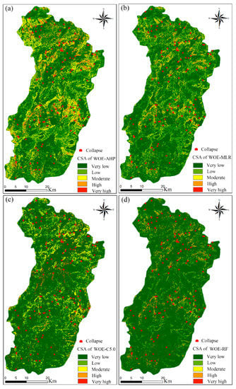
Figure 7.
Collapse susceptibility maps of (a) weight of evidence (WOE)-Analytic Hierarchy Process (AHP), (b) WOE-Multiple Linear Regression (MLR), (c) WOE-C5.0 and (d) WOE-Random Forest (RF).
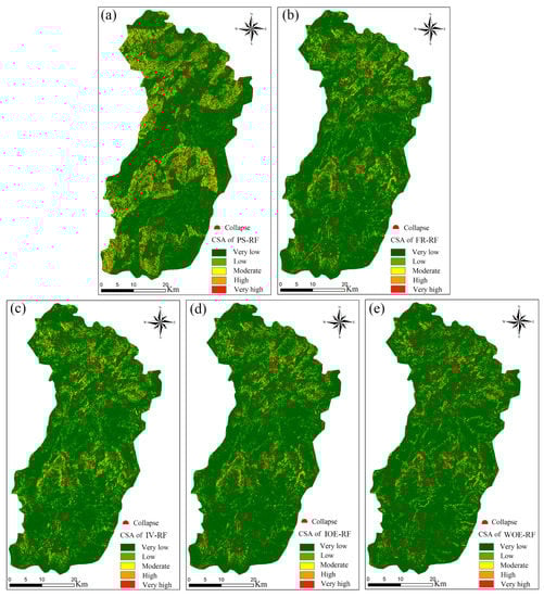
Figure 8.
Collapse susceptibility maps of (a) Probability Statistics (PSs)-RF, (b) Frequency Ratio (FR)-RF, (c) Information Value (IV)-RF, (d) Index of Entropy (IOE)-RF and (e) WOE-RF.
5. Uncertainty Analysis
5.1. Accuracy Analysis of ROC
The ROC statistical method was used to evaluate the prediction accuracies of samples in the testing set. In order to further quantify the CSP performance of different models, the AUC value was used as a specific evaluation index. The larger the AUC value is, the better the CSP performance of the model is. The ROC curves under all the coupled conditions are shown in Figure 9. The WOE-RF model has the highest prediction accuracy with an AUC value of 0.959. Furthermore, WOE shows the best predictive accuracy compared with other connection methods in the same data-based model, and the results of IOE, IV and FR are relatively consistent, followed by the PS-based model as shown in Table 4. Meanwhile, it is proved that the RF model has better prediction accuracy than the other data-based models in the CSP under all the connect methods. Furthermore, compared with traditional MLR and heuristic models, the AUC of the machine learning model was improved by about 0.1 (Figure 9).
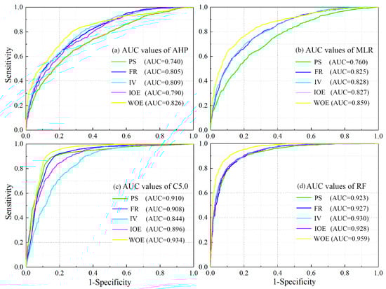
Figure 9.
ROC curves of collapse modeling based on the connection methods and data-based models: (a) AHP, (b) MLR, (c) C5.0 and (d) RF models.
Table 4.
Area under the ROC curve (AUC) values of different connection methods under different data-based models.
5.2. Distribution Rule of Collapse Susceptibility Index
The mean value and SD were used to reflect the average level and dispersion degree of CSI distribution, respectively, and then the uncertainties of CSIs under coupled conditions were analyzed.
(1) The distribution rules of the CSIs calculated by the WOE-based models are discussed as shown in Table 5 and Figure 10; meanwhile, the distribution rules of the CSIs under the other coupled models are similar to those of WOE-based models. The CSIs of the WOE-based models are ranked by the mean value as follows: Mean (WOE-AHP) > Mean (WOE-MLR) > Mean (WOE-C5.0) > Mean (WOE-RF). Among them, the CSIs of WOE-AHP and WOE-MLR models are normally distributed and mostly concentrate in the moderate levels, indicating that the CSIs predicted by WOE-AHP and WOE-MLR models are generally large. Combined with the AUC values of these coupled models, it can be seen that the abilities of the AHP and MLR models to identify collapse susceptibility are low. Moreover, the CSIs of RF and C5.0 models have similar distribution rules, which are concentrated in the very low and low levels, and gradually decrease in the other levels. In addition, the dispersion degree of these four models is exactly opposite to its mean value as follows: SD (WOE-RF) > SD (WOE-C5.0) > SD (WOE-MLR) > SD (WOE-AHP). The results show that RF and C5.0 models have a good differentiation degree for the CSIs of the region, and can well reflect the differences of the CSIs in different grid units. Moreover, fewer high CSIs were used to reflect as much known collapses as possible, which indirectly indicates that advanced machine learning models can predict the collapse susceptibility more effectively.
Table 5.
Mean and standard deviation of different connection methods under different data-based models.
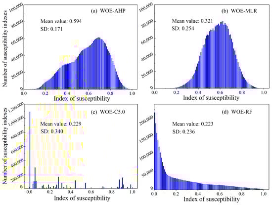
Figure 10.
Collapse susceptibility indexes distribution of WOE-AHP (a), WOE-MLR (b), WOE-C5.0 (c) and WOE-RF (d).
(2) Taking RF model as an example, the distribution rules of the CSIs predicted by different collection methods was analyzed, as shown in Table 5 and Figure 11. The mean value ranking of the CSIs of different connection methods is: Mean (WOE-RF) > Mean (IOE-RF) > Mean (FR-RF) > Mean (IV-RF) > Mean (PS-RF). The ranking of the SD is: SD (PS-RF) > SD (WOE-RF) > SD (IOE-RF) > SD (FR-RF) > SD (IV-RF). From the above comparisons, it can be seen that the mean value of the CSIs of the WOE connection method is the lowest, with a large SD. The CSIs results of IOE-, FR- and IV-based machine learning models are consistent, while the PS-based machine learning models exhibit the worst CSP performances with the highest means and the lowest SDs. Under all kinds of connect methods, the CSIs of C5.0, MLR and AHP all show almost the same CSP rules as the RF model.
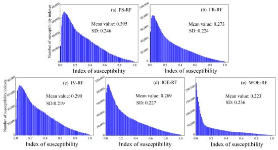
Figure 11.
Collapse susceptibility indexes distribution of PS-RF (a), FR-RF (b), IV-RF(c), IOE-RF (d) and WOE-RF (e).
5.3. Difference Significance Analysis of the CPS Results
The significant difference level and mean rank were used to further analyze the uncertainties of the CSP models coupled with the collection methods and data-based models. Specifically, the Friedman two-factor ANOVA analysis and test method by rank were used to test the difference significance of the CSIs predicted under the conditions of any two groups of different connection methods and data-based models. If the significance of the test results is less than 0.05, the CSIs of the two groups is significantly different, and the null hypothesis is rejected (there is no difference between the CSIs in the groups). Through the significance test of paired factors, the probability values of a hypothesis (p-values) were found to all be less than 0.05, with significant differences. Therefore, it was necessary to cross-verify the connection methods and the data-based models.
At the same time, this test was also used to calculate the mean ranks of CSIs predicted by the models coupled with the collection method and the data-based model, and to rank the performance of the coupled CSP models. If the average rank is smaller, the model performance will be better. The comparison results of any pair of models in the group are shown in Table 6. WOE-RF has a mean rank of 4.82, ranking the highest, followed by the WOE-C5.0 (5.30), and other WOE-based models. The CSP performances of the FR-based, IV-based and IOE-based machine learning models are consistent, while the PS-AHP model ranks as the worst. The significance difference level and the mean rank indicate the uncertainty features of the coupled collection methods and data-based models. Avoiding these uncertainties is important for obtaining reliable and stable CSP results.
Table 6.
Mean rank of different connection methods under different data-based models.
6. Discussion
6.1. CSP Modeling under Different Collection Methods
The impact degrees of each attribute interval of the environmental factors on the collapse susceptibility were quantitatively calculated by connection methods, which were used as the input variables of the data-based models to predict the spatial probability of collapse occurrence. In the classification processes of attribute intervals of environmental factors under different connection methods, the WOE can more effectively reflect the effects of spatial information on collapse than the other four connection methods and has a better prediction accuracy. Compared with IV and IOE methods, FR is more intuitive, which can guarantee the prediction accuracy and effectively avoid too complicated statistical calculations. The PS method reflects the contribution rate of collapse to the attribute interval, but fails to fully reflect the spatial correlations between collapses and attribute intervals of environmental factors. The more fully the correlation expression of spatial information between environmental factors and collapse, the greater the degree of differentiation of the CSIs, and the better the effect of CSP modeling. Furthermore, for the five nonlinear connection methods of PS, FR, IV, IOE and WOE, the mean values of the CSIs calculated by the coupled the data-based models decrease gradually, while the corresponding SD values increase gradually; meanwhile, the change trend of mean ranks of CSIs calculated by the coupled the data-based models are the same as the rules of mean values, and it can be seen that the modeling performance of the five collection methods become better and better when using PS, FR, IV and IOE to WOE methods.
6.2. CSP Modeling under Different Data-Based Models
Under the coupled conditions of the same connection method and different data-based models, the prediction accuracies of all coupled models show a consistent rule: AUCRF > AUC C5.0 > AUC MLR > AUC AHP, which shows that the prediction accuracies of machine learning models are higher than that of a conventional regression model and heuristic model. Analysis of the characteristics of CSIs: the CSIs predicted by the RF model are exponentially distributed (Figure 11), and the mean value of CSIs are in the transition zone between very low and low levels; the CSIs predicted by the C5.0 model are relatively discrete and these mean values are only higher than RF; however, the CSIs predicted by MLR and AHP tend to be normally distributed, with large mean values and in the moderate level, as shown in Figure 10. Compared with a conventional heuristic model and linear regression model, the CSIs predicted by machine learning models are more centralized in terms of distribution in very low and low levels. Meanwhile, the machine learning models are more accurate in predicting very high and high levels, and most historical collapse events fall in these levels. In addition, the SD values of the CSIs predicted by the MLR and AHP are smaller than those predicted by the machine learning models, which indicates that the CSIs obtained by MLR and AHP are not differentiated enough and the prediction accuracy is poor. As a whole, the AHP, MLR, C5.0 and RF models exhibit better prediction performances in turn from the characteristics of CSIs and prediction accuracy, as shown in Section 6.4.
6.3. CSP Modeling under Coupled Conditions of Connection Methods and Data-Based Models
From the perspective of the coupled models, the CSP accuracy of the WOE-RF model is the best, while that of the PS-AHP model is the worst. In addition, the PS-RF model can also achieve good CSP accuracy (AUC = 0.923). Compared with heuristic models and linear statistical models, machine learning models have stronger robustness in noise environments, can fully and efficiently mine incomplete information and the training and testing effects of CSP modeling are excellent [90]. Furthermore, the RF model is more stable and has more advantages than the C5.0 DT model. Heuristics and statistical models rely on the collection methods, and the more obvious the statistical rule of collection methods, the better the prediction accuracy [6].
RF is a supervised integrated learning algorithm based on a decision tree, which is more accurate than individual algorithms such as C5.0 and MLR. Due to out-of-pocket data, unbiased estimation of true error is obtained in the process of model generation without loss of training data. With the introduction of sample and characteristic randomness, RF has certain anti-noise and anti-overfitting ability in the testing process. As a combination of multiple classification trees, RF can process nonlinear data and high-dimensional data without making a feature selection. Meanwhile, RF can process both discrete and continuous data with strong adaptability to datasets, so it is suitable to be used as a nonlinear classification model.
Friedman analysis and test method were used to verify the difference of CSP performance of coupled models. The CSIs predicted by of WOE-based models are significantly different from those predicted by the coupled of other connection methods and the data-based models. Compared with the other data-based coupled models, the CSP performance of the RF model coupled with the five collection methods has a significant difference. Moreover, the WOE-RF model exhibits the best CSP performance, with the lowest mean rank and the best predicted accuracy. The results of this study can guide the selection of the best combination of collapse connection methods and data-based models in other research areas. Although these results are obtained in the areas with mountainous and hilly terrains, they can be generalized to other regions as a guideline or alternative method for selecting the best combination.
6.4. CSP Modeling under Single Data-Based Models with No Connect Methods
This paper also conducts CSP modeling based on the original continuous environment factors data without the connection method. That is to say, the original continuous environment factors data were directly used as input variables of the four types of data-based models. Then, these models were trained and tested based on the appropriate parameters similar to the above model, respectively. The prediction accuracy of these single data-based models with no connect methods were slightly lower than those of the coupling model using the connection method (Figure 12 and Figure 13). In addition, the distribution rule of the collapse susceptibility maps created by the coupling models and single models were similar as a whole. In order to improve the modeling efficiency of CSP, a single machine learning model can be used directly. However, in order to better reflect the spatial correlations between the collapse distribution and basic environmental factors or to analyze the influence rules of each subinterval of environmental factors on the evolution of collapses, the coupling models considering the connection method need to be adopted.
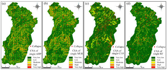
Figure 12.
Collapse susceptibility maps produced by single data-based models considering original environmental factors as model input variables: (a) CSA of single AHP, (b) CSA of single MLR, (c) CSA of single C5.0, (d) CSA of single RF model.
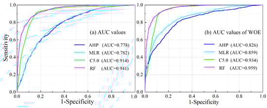
Figure 13.
ROC curves of (a) data-based models and (b) WOE-based models.
7. Conclusions
Some uncertainty problems in CSP modeling, such as nonlinear correlation methods coupled with data-based models to obtain the optimal coupled conditions, are very important for predicting the accurate and reliable CSMs. This paper discusses these uncertainties in depth and comes to the following conclusions:
- (1)
- Compared with the other four connection methods, WOE better reflects the nonlinear correlation between collapse and related environmental factors and has a better spatial information discrimination ability regarding environmental factors. Compared with the CSP modeling based on the FR, IV and IOE, the CSP accuracies of the WOE-based models are the highest, with the lowest mean values, average ranks and larger SDs. Meanwhile, the CSP accuracies of the three types of the FR, IV and IOE connection methods tend to be consistent, and their CSP performances are not as good as those of the WOE-based models. In addition, the prediction results of PS-based models are poor.
- (2)
- Compared with other kinds of data-based models, the RF model has the highest CSP accuracy, with the lowest mean value and mean rank of the CSIs and a larger SD, followed by the C5.0, MLR and AHP models. It can be seen that the advanced machine learning models can effectively improve the CSP accuracy, and the collapse susceptibility identification ability is significant.
- (3)
- Under the coupled conditions of different collection methods and data-based models, the CSP accuracy of the WOE-RF model is the highest with the lowest mean value and mean rank. The predicted CSIs of WOE-RF model is more in line with the actual characteristics of collapse probability distribution than the other coupled models. On the contrary, the PS-AHP model has the lowest prediction accuracy with a larger mean value and mean rank and smaller SD value.
- (4)
- In general, the CSP performance of single data-based models not considering connect methods was slightly worse than those of the connection method-based models. The comparison results further demonstrate the importance of spatial correlation analysis of environmental factors for CSP modeling.
- (5)
- Although this study mainly analyzes the uncertainty rules of CSP modeling under the conditions of different data-based models and connections between collapses and environmental factors, the conclusions of this study also have some reference values for other kinds of geological disasters’ (landslide, debris flow, etc.) susceptibility predictions. This is because the evolution processes of these geological disasters are closely related to various environmental factors in the spatial perspective.
Author Contributions
Conceptualization, W.L. and F.H.; Data curation, W.L.; Formal analysis, W.L.; Funding acquisition, F.H.; Investigation, Z.G.; Methodology, W.L.; Project administration, F.H.; Resources, W.L. and F.H.; Software, W.L.; Supervision, F.H.; Validation, F.H.; Writing—original draft, W.L. and F.H.; Writing—review and editing, X.F., W.C., H.H. and J.H. All authors have read and agreed to the published version of the manuscript.
Funding
This research is funded by the Natural Science Foundation of China (No. 41807285, 41867036 and 51679117), the China Postdoctoral Science Foundation (No. 2019M652287 and 2020T130274), the Jiangxi Provincial Natural Science Foundation (No. 20192BAB216034) and the and the Jiangxi Provincial Postdoctoral Science Foundation (No. 2019KY08).
Conflicts of Interest
The authors declare no conflict of interest.
References
- Boualla, O.; Mehdi, K.; Zourarah, B. Collapse dolines susceptibility mapping in doukkala abda (western morocco) by using gis matrix method (gmm). Modeling Earth Syst. Environ. 2016, 2, 9. [Google Scholar] [CrossRef]
- Li, Y.; Sheng, Y.; Chai, B.; Zhang, W.; Zhang, T.; Wang, J. Collapse susceptibility assessment using a support vector machine compared with back-propagation and radial basis function neural networks. Geomat. Nat. Hazards Risk 2020, 11, 510–534. [Google Scholar] [CrossRef]
- Liang, C.; Jaksa, M.B.; Kuo, Y.L.; Ostendorf, B. Identifying areas susceptible to high risk of riverbank collapse along the lower river murray. Comput. Geotech. 2015, 69, 236–246. [Google Scholar] [CrossRef]
- Martínez-Moreno, F.J.; Galindo-Zaldívar, J.; González-Castillo, L.; Azañón, J.M. Collapse susceptibility map in abandoned mining areas by microgravity survey: A case study in candado hill (Málaga, southern Spain). J. Appl. Geophys. 2016, 130, 101–109. [Google Scholar] [CrossRef]
- Santo, A.; Budetta, P.; Forte, G.; Marino, E.; Pignalosa, A. Karst collapse susceptibility assessment: A case study on the Amalfi coast (southern Italy). Geomorphology 2017, 285, 247–259. [Google Scholar] [CrossRef]
- Hong, H.; Miao, Y.; Liu, J.; Zhu, A.X. Exploring the effects of the design and quantity of absence data on the performance of random forest-based landslide susceptibility mapping. Catena 2019, 176, 45–64. [Google Scholar] [CrossRef]
- Huang, F.; Zhang, J.; Zhou, C.; Wang, Y.; Huang, J.; Zhu, L. A deep learning algorithm using a fully connected sparse autoencoder neural network for landslide susceptibility prediction. Landslides 2020, 17, 217–229. [Google Scholar] [CrossRef]
- Di Napoli, M.; Marsiglia, P.; Di Martire, D.; Ramondini, M.; Ullo, S.L.; Calcaterra, D. Landslide susceptibility assessment of wildfire burnt areas through earth-observation techniques and a machine learning-based approach. Remote Sens. 2020, 12, 2505. [Google Scholar] [CrossRef]
- Tien Bui, D.; Shahabi, H.; Shirzadi, A.; Chapi, K.; Alizadeh, M.; Chen, W.; Mohammadi, A.; Ahmad, B.B.; Panahi, M.; Hong, H.; et al. Landslide detection and susceptibility mapping by airsar data using support vector machine and index of entropy models in cameron highlands, Malaysia. Remote Sens. 2018, 10, 1527. [Google Scholar] [CrossRef]
- Chang, Z.; Du, Z.; Zhang, F.; Huang, F.; Chen, J.; Li, W.; Guo, Z. Landslide susceptibility prediction based on remote sensing images and gis: Comparisons of supervised and unsupervised machine learning models. Remote Sens. 2020, 12, 502. [Google Scholar] [CrossRef]
- Huang, F.; Chen, L.; Yin, K.; Huang, J.; Gui, L. Object-oriented change detection and damage assessment using high-resolution remote sensing images, tangjiao landslide, three gorges reservoir, China. Environ. Earth Sci. 2018, 77, 183. [Google Scholar] [CrossRef]
- Chen, W.; Hong, H.; Panahi, M.; Shahabi, H.; Wang, Y.; Shirzadi, A.; Pirasteh, S.; Alesheikh, A.A.; Khosravi, K.; Panahi, S. Spatial prediction of landslide susceptibility using gis-based data mining techniques of anfis with whale optimization algorithm (woa) and grey wolf optimizer (gwo). Appl. Sci. 2019, 9, 3755. [Google Scholar] [CrossRef]
- Sahin, E.K.; Colkesen, I.; Kavzoglu, T. A comparative assessment of canonical correlation forest, random forest, rotation forest and logistic regression methods for landslide susceptibility mapping. Geocarto Int. 2020, 35, 341–363. [Google Scholar] [CrossRef]
- Chen, W.; Chen, X.; Peng, J.; Panahi, M.; Lee, S. Landslide susceptibility modeling based on anfis with teaching-learning-based optimization and satin bowerbird optimizer. Geosci. Front. 2021, 12, 93–107. [Google Scholar] [CrossRef]
- Garosi, Y.; Sheklabadi, M.; Conoscenti, C.; Pourghasemi, H.R.; Van Oost, K. Assessing the performance of gis- based machine learning models with different accuracy measures for determining susceptibility to gully erosion. Sci. Total Environ. 2019, 664, 1117–1132. [Google Scholar] [CrossRef]
- Costache, R.; Hong, H.; Pham, Q.B. Comparative assessment of the flash-flood potential within small mountain catchments using bivariate statistics and their novel hybrid integration with machine learning models. Sci. Total Environ. 2020, 711, 134514. [Google Scholar] [CrossRef]
- Kavoura, K.; Sabatakakis, N. Investigating landslide susceptibility procedures in greece. Landslides 2019, 17, 127–145. [Google Scholar] [CrossRef]
- Zhang, J.; Yin, K.; Wang, J. Evaluation of landslide susceptibility for wanzhou district of three gorges reservoir. Chin. J. Rock Mech. Eng. 2016, 35, 284–296. [Google Scholar]
- Demir, G. Gis-based landslide susceptibility mapping for a part of the north anatolian fault zone between reşadiye and koyulhisar (Turkey). Catena 2019, 183, 104211. [Google Scholar] [CrossRef]
- Huang, F.; Yao, C.; Liu, W.; Li, Y.; Liu, X. Landslide susceptibility assessment in the nantian area of china: A comparison of frequency ratio model and support vector machine. Geomat. Nat. Hazards Risk 2018, 9, 919–938. [Google Scholar] [CrossRef]
- Kim, H.G.; Lee, D.K.; Park, C.; Ahn, Y.; Kil, S.-H.; Sung, S.; Biging, G.S. Estimating landslide susceptibility areas considering the uncertainty inherent in modeling methods. Stoch. Environ. Res. Risk Assess. 2018, 32, 2987–3019. [Google Scholar] [CrossRef]
- Sun, Q.; Tang, Z.; Yuanyao, L.I.; Chai, B.; Jizhi, L.U. Susceptibility assessment of rock collapse hazards in longjuba area based on dummy variables analysis. Hydrogeol. Eng. Geol. 2017, 44, 127–135. [Google Scholar]
- Lombardo, L.; Opitz, T.; Huser, R. Numerical recipes for landslide spatial prediction using r-inla. In Spatial Modeling in Gis and R for Earth and Environmental Sciences; Elsevier: Amsterdam, The Netherlands, 2019; pp. 55–83. [Google Scholar]
- Bragagnolo, L.; Silva, R.V.D.; Grzybowski, J.M.V. Landslide susceptibility mapping with r.Landslide: A free open-source gis-integrated tool based on artificial neural networks. Environ. Model. Softw. 2020, 123, 104565. [Google Scholar] [CrossRef]
- Sepe, C.; Confuorto, P.; Angrisani, A.C.; Di Martire, D.; Di Napoli, M.; Calcaterra, D. Application of a statistical approach to landslide susceptibility map generation in urban settings. In Iaeg/Aeg Annual Meeting Proceedings, San Francisco, California, 2018—Volume 1; Springer: Cham, Switzerland, 2019; pp. 155–162. [Google Scholar]
- Huang, F.; Huang, J.; Jiang, S.; Zhou, C. Landslide displacement prediction based on multivariate chaotic model and extreme learning machine. Eng. Geol. 2017, 218, 173–186. [Google Scholar] [CrossRef]
- Reichenbach, P.; Rossi, M.; Malamud, B.D.; Mihir, M.; Guzzetti, F. A review of statistically-based landslide susceptibility models. Earth Sci. Rev. 2018, 180, 60–91. [Google Scholar] [CrossRef]
- Adnan, M.S.G.; Rahman, M.S.; Ahmed, N.; Ahmed, B.; Rabbi, M.F.; Rahman, R.M. Improving spatial agreement in machine learning-based landslide susceptibility mapping. Remote Sens. 2020, 12, 3347. [Google Scholar] [CrossRef]
- Devkota, K.C.; Regmi, A.D.; Pourghasemi, H.R.; Yoshida, K.; Pradhan, B.; Ryu, I.C.; Dhital, M.R.; Althuwaynee, O.F. Landslide susceptibility mapping using certainty factor, index of entropy and logistic regression models in gis and their comparison at mugling–narayanghat road section in nepal himalaya. Nat. Hazards 2012, 65, 135–165. [Google Scholar] [CrossRef]
- Dao, D.V.; Jaafari, A.; Bayat, M.; Mafi-Gholami, D.; Qi, C.; Moayedi, H.; Phong, T.V.; Ly, H.-B.; Le, T.-T.; Trinh, P.T.; et al. A spatially explicit deep learning neural network model for the prediction of landslide susceptibility. Catena 2020, 188, 104451. [Google Scholar] [CrossRef]
- Huang, F.; Cao, Z.; Guo, J.; Jiang, S.-H.; Li, S.; Guo, Z. Comparisons of heuristic, general statistical and machine learning models for landslide susceptibility prediction and mapping. Catena 2020, 191, 104580. [Google Scholar] [CrossRef]
- Iglesias, R.; Fabregas, X.; Aguasca, A.; Mallorqui, J.J.; Lopez-Martinez, C.; Gili, J.A.; Corominas, J. Atmospheric phase screen compensation in ground-based sar with a multiple-regression model over mountainous regions. IEEE Trans. Geosci. Remote Sens. 2014, 52, 2436–2449. [Google Scholar] [CrossRef]
- Saha, S.; Saha, M.; Mukherjee, K.; Arabameri, A.; Ngo, P.T.T.; Paul, G.C. Predicting the deforestation probability using the binary logistic regression, random forest, ensemble rotational forest, reptree: A case study at the gumani river basin, india. Sci. Total Environ. 2020, 730, 139197. [Google Scholar] [CrossRef] [PubMed]
- Dou, J.; Yunus, A.P.; Merghadi, A.; Shirzadi, A.; Nguyen, H.; Hussain, Y.; Avtar, R.; Chen, Y.; Pham, B.T.; Yamagishi, H. Different sampling strategies for predicting landslide susceptibilities are deemed less consequential with deep learning. Sci. Total Environ. 2020, 720, 137320. [Google Scholar] [CrossRef] [PubMed]
- Huang, F.; Yin, K.; Huang, J.; Gui, L.; Wang, P. Landslide susceptibility mapping based on self-organizing-map network and extreme learning machine. Eng. Geol. 2017, 223, 11–22. [Google Scholar] [CrossRef]
- Zhu, L.; Huang, L.; Fan, L.; Huang, J.; Huang, F.; Chen, J.; Zhang, Z.; Wang, Y. Landslide susceptibility prediction modeling based on remote sensing and a novel deep learning algorithm of a cascade-parallel recurrent neural network. Sensors 2020, 20, 1576. [Google Scholar] [CrossRef]
- Zhao, X.; Chen, W. Optimization of Computational Intelligence Models for Landslide Susceptibility Evaluation. Remote Sens. 2020, 12, 2180. [Google Scholar] [CrossRef]
- Li, D.; Huang, F.; Yan, L.; Cao, Z.; Chen, J.; Ye, Z. Landslide susceptibility prediction using particle-swarm-optimized multilayer perceptron: Comparisons with multilayer-perceptron-only, bp neural network, and information value models. Appl. Sci. 2019, 9, 3664. [Google Scholar] [CrossRef]
- Park, S.-J.; Lee, C.-W.; Lee, S.; Lee, M.-J. Landslide susceptibility mapping and comparison using decision tree models: A case study of jumunjin area, korea. Remote Sens. 2018, 10, 1545. [Google Scholar] [CrossRef]
- Arabameri, A.; Saha, S.; Roy, J.; Chen, W.; Blaschke, T.; Tien Bui, D. Landslide susceptibility evaluation and management using different machine learning methods in the Gallicash River Watershed, Iran. Remote Sens. 2020, 12, 475. [Google Scholar] [CrossRef]
- Chen, W.; Zhao, X.; Tsangaratos, P.; Shahabi, H.; Ilia, I.; Xue, W.; Wang, X.; Ahmad, B.B. Evaluating the usage of tree-based ensemble methods in groundwater spring potential mapping. J. Hydrol. 2020, 583, 124602. [Google Scholar] [CrossRef]
- Trigila, A.; Iadanza, C.; Esposito, C.; Scarascia-Mugnozza, G. Comparison of logistic regression and random forests techniques for shallow landslide susceptibility assessment in Giampilieri (NE Sicily, Italy). Geomorphology 2015, 249, 119–136. [Google Scholar] [CrossRef]
- Huang, F.; Huang, J.; Jiang, S.-H.; Zhou, C. Prediction of groundwater levels using evidence of chaos and support vector machine. J. Hydroinformatics 2017, 19, 586–606. [Google Scholar] [CrossRef]
- Kalantar, B.; Ueda, N.; Saeidi, V.; Ahmadi, K.; Halin, A.A.; Shabani, F. Landslide susceptibility mapping: Machine and ensemble learning based on remote sensing big data. Remote Sens. 2020, 12, 1737. [Google Scholar] [CrossRef]
- He, Q.; Shahabi, H.; Shirzadi, A.; Li, S.; Chen, W.; Wang, N.; Chai, H.; Bian, H.; Ma, J.; Chen, Y.; et al. Landslide spatial modelling using novel bivariate statistical based naive bayes, rbf classifier, and rbf network machine learning algorithms. Sci. Total Environ. 2019, 663, 1–15. [Google Scholar] [CrossRef] [PubMed]
- Wang, L.-J.; Guo, M.; Sawada, K.; Lin, J.; Zhang, J. Landslide susceptibility mapping in mizunami city, Japan: A comparison between logistic regression, bivariate statistical analysis and multivariate adaptive regression spline models. Catena 2015, 135, 271–282. [Google Scholar] [CrossRef]
- Sun, D.; Wen, H.; Wang, D.; Xu, J. A random forest model of landslide susceptibility mapping based on hyperparameter optimization using bayes algorithm. Geomorphology 2020, 362, 107201. [Google Scholar] [CrossRef]
- Liu, W.; Luo, X.; Huang, F.; Fu, M. Prediction of soil water retention curve using bayesian updating from limited measurement data. Appl. Math. Model. 2019, 76, 380–395. [Google Scholar] [CrossRef]
- Yilmaz, I.; Marschalko, M.; Bednarik, M. An assessment on the use of bivariate, multivariate and soft computing techniques for collapse susceptibility in gis environ. J. Earth Syst. Sci. 2013, 122, 371–388. [Google Scholar] [CrossRef][Green Version]
- Chen, W.; Li, Y. Gis-based evaluation of landslide susceptibility using hybrid computational intelligence models. Catena 2020, 195, 104777. [Google Scholar] [CrossRef]
- Chen, X.; Chen, W. Gis-based landslide susceptibility assessment using optimized hybrid machine learning methods. Catena 2021, 196, 104833. [Google Scholar] [CrossRef]
- Chen, W.; Chen, Y.; Tsangaratos, P.; Ilia, I.; Wang, X. Combining evolutionary algorithms and machine learning models in landslide susceptibility assessments. Remote Sens. 2020, 12, 3854. [Google Scholar] [CrossRef]
- Du, J.; Glade, T.; Woldai, T.; Chai, B.; Zeng, B. Landslide susceptibility assessment based on an incomplete landslide inventory in the Jilong Valley, Tibet, Chinese Himalayas. Eng. Geol. 2020, 270, 105572. [Google Scholar] [CrossRef]
- Gayen, A.; Pourghasemi, H.R.; Saha, S.; Keesstra, S.; Bai, S. Gully erosion susceptibility assessment and management of hazard-prone areas in india using different machine learning algorithms. Sci. Total Environ. 2019, 668, 124–138. [Google Scholar] [CrossRef] [PubMed]
- Huang, F.; Yin, K.; Zhang, G.; Gui, L.; Yang, B.; Liu, L. Landslide displacement prediction using discrete wavelet transform and extreme learning machine based on chaos theory. Environ. Earth Sci. 2016, 75, 1376. [Google Scholar] [CrossRef]
- Shahabi, H.; Khezri, S.; Ahmad, B.B.; Hashim, M. Landslide susceptibility mapping at central zab basin, Iran: A comparison between analytical hierarchy process, frequency ratio and logistic regression models. Catena 2014, 115, 55–70. [Google Scholar] [CrossRef]
- Shirzadi, A.; Solaimani, K.; Roshan, M.H.; Kavian, A.; Chapi, K.; Shahabi, H.; Keesstra, S.; Ahmad, B.B.; Bui, D.T. Uncertainties of prediction accuracy in shallow landslide modeling: Sample size and raster resolution. Catena 2019, 178, 172–188. [Google Scholar] [CrossRef]
- Huang, F.; Chen, J.; Yao, C.; Chang, Z.; Jiang, Q.; Li, S.; Guo, Z. Susle: A slope and seasonal rainfall-based rusle model for regional quantitative prediction of soil erosion. Bull. Eng. Geol. Environ. 2020, 79, 5213–5228. [Google Scholar] [CrossRef]
- Huang, F.; Yin, K.; He, T. Analysis of influence factors and displacement prediction of reservoir landslide-a case study of three gorges reservoir. China 2016, 23, 617–626. [Google Scholar]
- Rabby, Y.W.; Ishtiaque, A.; Rahman, M.S. Evaluating the effects of digital elevation models in landslide susceptibility mapping in rangamati district, bangladesh. Remote Sens. 2020, 12, 2718. [Google Scholar] [CrossRef]
- Jiang, S.-H.; Huang, J.; Huang, F.; Yang, J.; Yao, C.; Zhou, C.-B. Modelling of spatial variability of soil undrained shear strength by conditional random fields for slope reliability analysis. Appl. Math. Model. 2018, 63, 374–389. [Google Scholar] [CrossRef]
- Jiang, Y.; Liao, M.; Zhou, Z.; Shi, X.; Zhang, L.; Balz, T. Landslide deformation analysis by coupling deformation time series from sar data with hydrological factors through data assimilation. Remote Sens. 2016, 8, 179. [Google Scholar] [CrossRef]
- Huang, F.; Luo, X.; Liu, W. Stability analysis of hydrodynamic pressure landslides with different permeability coefficients affected by reservoir water level fluctuations and rainstorms. Water 2017, 9, 450. [Google Scholar] [CrossRef]
- Liu, W.; Song, X.; Huang, F.; Hu, L. Experimental study on the disintegration of granite residual soil under the combined influence of wetting–drying cycles and acid rain. Geomat. Nat. Hazards Risk 2019, 10, 1912–1927. [Google Scholar] [CrossRef]
- Roy, J.; Saha, S.; Arabameri, A.; Blaschke, T.; Bui, D.T. A novel ensemble approach for landslide susceptibility mapping (lsm) in darjeeling and kalimpong districts, west bengal, India. Remote Sens. 2019, 11, 2866. [Google Scholar] [CrossRef]
- Nachappa, T.G.; Ghorbanzadeh, O.; Gholamnia, K.; Blaschke, T. Multi-hazard exposure mapping using machine learning for the state of salzburg, Austria. Remote Sens. 2020, 12, 2757. [Google Scholar] [CrossRef]
- Cantarino, I.; Carrion, M.A.; Goerlich, F.; Martinez Ibañez, V. A roc analysis-based classification method for landslide susceptibility maps. Landslides 2018, 16, 265–282. [Google Scholar] [CrossRef]
- Juliev, M.; Mergili, M.; Mondal, I.; Nurtaev, B.; Pulatov, A.; Hubl, J. Comparative analysis of statistical methods for landslide susceptibility mapping in the bostanlik district, uzbekistan. Sci. Total Environ. 2019, 653, 801–814. [Google Scholar] [CrossRef]
- Azareh, A.; Rahmati, O.; Rafiei-Sardooi, E.; Sankey, J.B.; Lee, S.; Shahabi, H.; Ahmad, B.B. Modelling gully-erosion susceptibility in a semi-arid region, iran: Investigation of applicability of certainty factor and maximum entropy models. Sci. Total Environ. 2019, 655, 684–696. [Google Scholar] [CrossRef]
- Pourghasemi, H.R.; Pradhan, B.; Gokceoglu, C. Application of fuzzy logic and analytical hierarchy process (ahp) to landslide susceptibility mapping at haraz watershed, Iran. Nat. Hazards 2012, 63, 965–996. [Google Scholar] [CrossRef]
- Ma, J.; Tang, H.; Liu, X.; Hu, X.; Sun, M.; Song, Y. Establishment of a deformation forecasting model for a step-like landslide based on decision tree c5.0 and two-step cluster algorithms: A case study in the three gorges reservoir area, China. Landslides 2017, 14, 1275–1281. [Google Scholar] [CrossRef]
- Huang, F.; Chen, J.; Du, Z.; Yao, C.; Huang, J.; Jiang, Q.; Chang, Z.; Li, S. Landslide susceptibility prediction considering regional soil erosion based on machine-learning models. Isprs Int. J. Geo-Inf. 2020, 9, 377. [Google Scholar] [CrossRef]
- Wang, Y.; Tang, H.; Wen, T.; Ma, J.; Zou, Z.; Xiong, C. Point and interval predictions for tanjiahe landslide displacement in the three gorges reservoir area, China. Geofluids 2019, 2019, 1–14. [Google Scholar] [CrossRef]
- Khosravi, K.; Pham, B.T.; Chapi, K.; Shirzadi, A.; Shahabi, H.; Revhaug, I.; Prakash, I.; Tien Bui, D. A comparative assessment of decision trees algorithms for flash flood susceptibility modeling at Haraz watershed, northern Iran. Sci. Total Environ. 2018, 627, 744–755. [Google Scholar] [CrossRef] [PubMed]
- Yeon, Y.-K.; Han, J.-G.; Ryu, K.H. Landslide susceptibility mapping in injae, korea, using a decision tree. Eng. Geol. 2010, 116, 274–283. [Google Scholar] [CrossRef]
- Vakhshoori, V.; Zare, M. Is the roc curve a reliable tool to compare the validity of landslide susceptibility maps. Geomat. Nat. Hazards Risk 2018, 9, 249–266. [Google Scholar] [CrossRef]
- Corsini, A.; Mulas, M. Use of roc curves for early warning of landslide displacement rates in response to precipitation (Piagneto Landslide, Northern Apennines, Italy). Landslides 2017, 14, 1241–1252. [Google Scholar] [CrossRef]
- Sezer, E.A.; Nefeslioglu, H.A.; Osna, T. An expert-based landslide susceptibility mapping (lsm) module developed for netcad architect software. Comput. Geosci. 2017, 98, 26–37. [Google Scholar] [CrossRef]
- Almeida, S.; Holcombe, E.A.; Pianosi, F.; Wagener, T. Dealing with deep uncertainties in landslide modelling for disaster risk reduction under climate change. Nat. Hazards Earth Syst. Sci. 2017, 17, 225–241. [Google Scholar] [CrossRef]
- Romer, C.; Ferentinou, M. Shallow landslide susceptibility assessment in a semiarid environment—A quaternary catchment of KwaZulu-Natal, South Africa. Eng. Geol. 2016, 201, 29–44. [Google Scholar] [CrossRef]
- Huang, F.; Cao, Z.; Jiang, S.-H.; Zhou, C.; Huang, J.; Guo, Z. Landslide susceptibility prediction based on a semi-supervised multiple-layer perceptron model. Landslides 2020, 17, 2919–2930. [Google Scholar] [CrossRef]
- Huang, F.; Yang, J.; Zhang, B.; Li, Y.; Huang, J.; Chen, N. Regional terrain complexity assessment based on principal component analysis and geographic information system: A case of Jiangxi province, China. Isprs Int. J. Geo-Inf. 2020, 9, 539. [Google Scholar] [CrossRef]
- Pisano, L.; Zumpano, V.; Malek, Z.; Rosskopf, C.M.; Parise, M. Variations in the susceptibility to landslides, as a consequence of land cover changes: A look to the past, and another towards the future. Sci. Total Environ. 2017, 601–602, 1147–1159. [Google Scholar] [CrossRef] [PubMed]
- Liu, W.; Wan, S.; Huang, F.; Luo, X.; Fu, M. Experimental study of subsurface erosion in granitic under the conditions of different soil column angles and flow discharges. Bull. Eng. Geol. Environ. 2019, 78, 5877–5888. [Google Scholar] [CrossRef]
- Chang, Z.; Gao, H.; Huang, F.; Chen, J.; Huang, J.; Guo, Z. Study on the creep behaviours and the improved burgers model of a loess landslide considering matric suction. Nat. Hazards 2020, 103, 1479–1497. [Google Scholar] [CrossRef]
- Li, Y.; Huang, J.; Jiang, S.H.; Huang, F.; Chang, Z. A web-based gps system for displacement monitoring and failure mechanism analysis of reservoir landslide. Sci. Rep. 2017, 7, 17171. [Google Scholar] [CrossRef]
- Guo, Z.; Yin, K.; Gui, L.; Liu, Q.; Huang, F.; Wang, T. Regional rainfall warning system for landslides with creep deformation in three gorges using a statistical black box model. Sci. Rep. 2019, 9, 8962. [Google Scholar] [CrossRef]
- Liu, W.; Luo, X.; Huang, F.; Fu, M. Uncertainty of the soil–water characteristic curve and its effects on slope seepage and stability analysis under conditions of rainfall using the markov chain monte carlo method. Water 2017, 9, 758. [Google Scholar] [CrossRef]
- Zhang, C.; Chen, Y.; Zhang, Y.; Sun, X. Geohazard susceptibility evaluation in zhaotong of yunnan based on the multivariate linear regression model. Hydrogeol. Eng. Geol. 2016, 43, 159–163. [Google Scholar]
- Pham, B.T.; Tien Bui, D.; Prakash, I.; Dholakia, M.B. Hybrid integration of multilayer perceptron neural networks and machine learning ensembles for landslide susceptibility assessment at Himalayan area (India) using gis. Catena 2017, 149, 52–63. [Google Scholar] [CrossRef]
Publisher’s Note: MDPI stays neutral with regard to jurisdictional claims in published maps and institutional affiliations. |
© 2020 by the authors. Licensee MDPI, Basel, Switzerland. This article is an open access article distributed under the terms and conditions of the Creative Commons Attribution (CC BY) license (http://creativecommons.org/licenses/by/4.0/).