Abstract
Lake water body extraction from remote sensing images is a key technique for spatial geographic analysis. It plays an important role in the prevention of natural disasters, resource utilization, and water quality monitoring. Inspired by the recent years of research in computer vision on fully convolutional neural networks (FCN), an end-to-end trainable model named the multi-scale lake water extraction network (MSLWENet) is proposed. We use ResNet-101 with depthwise separable convolution as an encoder to obtain the high-level feature information of the input image and design a multi-scale densely connected module to expand the receptive field of feature points by different dilation rates without increasing the computation. In the decoder, the residual convolution is used to abstract the features and fuse the features at different levels, which can obtain the final lake water body extraction map. Through visual interpretation of the experimental results and the calculation of the evaluation indicators, we can see that our model extracts the water bodies of small lakes well and solves the problem of large intra-class variance and small inter-class variance in the lakes’ water bodies. The overall accuracy of our model is up to 98.53% based on the evaluation indicators. Experimental results demonstrate that the MSLWENet, which benefits from the convolutional neural network, is an excellent lake water body extraction network.
1. Introduction
Lake water body extraction is a fundamental and important field of remote sensing image analysis. There are approximately 304 million natural lakes on the surface of the Earth, which are composed by millions of small water bodies, covering about 4.6 million kilometers of water [1]. With the crisis of global warming, lakes are very sensitive to global temperature changes and play an important role in the carbon cycle [2]. On the other hand, lakes also have the function of developing irrigation [3], providing a source of drinking water on which human life depends [4], and transportation [5]. Remote sensing images of lakes contain a great deal of information that can be used in other areas, such as disaster monitoring, the development of agriculture, livestock farming, and geographic planning. Therefore, it is important to study the automatic lake water body extraction from remote sensing images.
Since remote sensing image acquisition information is less affected by natural conditions, large area images can be acquired in a short time and at a low cost. Therefore, a large number of remote sensing images have been used for sea-land segmentation [6,7], water extraction [8,9,10,11,12,13,14,15,16,17,18,19], and other applications. In the recent years of research, numerous water extraction methods have been proposed, such as the threshold method [8,9,16,17,18], machine learning method [10,11,19], and deep learning method [12,13,14].
Remote sensing images use different bands and contain different information. The threshold method is widely used in the field of water extraction, which involves with the number of bands used, mainly single band [16] and multi-band [8,17]. The difference between the water bodies and non-water objects in the NIR band is the largest, and a single NIR band as the water index can be used to obtain satisfactory results for water bodies’ extraction [16]. The use of multi-band water index thresholding to extract water can make use of spectral information from different bands as much as possible, but can also result in redundancy. Since mountain shadows and cloud shadows have similar spectral characteristics as water bodies, a single, fixed threshold may lead to over- or under-segmentation of the water bodies [18]. Therefore, achieving dynamic adjustment of the threshold and producing optimal segmentation results are complex and time-consuming. Feyisa et al. [8] introduced an automatic water extraction index to improve classification accuracy in the presence of various environmental noises, including shadows and areas within dark surfaces that cannot be correctly classified by other classification methods. This method provides a stable threshold while improving accuracy. Zhang et al. [9] achieved automatic dynamic adjustment of thresholds, which reduced the dependence on data without degradation of the accuracy and could be applied in massive remote sensing images.
Methods based on spectral information provide a good result on low resolution multispectral images, but when applied to medium or high resolution images, they become less robust as more spatial detail becomes visible. With the development of machine learning algorithms, which use artificially designed features, traditional machine learning algorithms have shown strong robustness in water bodies’ extraction [10,11,19]. The water extraction methods can be classified as pixel-based [10] or object-based [19]. Zhang et al. [10] proposed a pixel area index to assist normalized differential water index detection of major water bodies, while using K-means clustering of water image elements near the boundary section to solve the complete boundary image element extraction problem, but there was still the problem of the optimal selection of the thresholds. Chen et al. [19] used object-oriented classification techniques combined with the spectral, textural, and geometric features of remote sensing images to extract information from the water bodies. Both the pixel-oriented and object-oriented methods of water extraction are lacking in the study of water body types. There are many methods for water extraction, but the research to determine its type based on water extraction is lacking [11]. Huang et al. [11] presented a two-level machine learning framework for identifying water types at the target level using geometric and textural features under pixel-based water extraction conditions, filling a gap in the research. Although machine learning based algorithms have achieved good results in remote sensing image analysis, they are limited by the artificial design of features to compute and stitch together, which are fed into support vector machines [20], random forests [21], etc, and are less adaptive to different datasets.
In the last decade, deep learning techniques have made significant breakthroughs in the field of image processing, such as semantic segmentation [22,23,24,25], object detection [26,27], and image classification [28,29,30]. Deep convolutional neural networks (DCNN) can automatically learn features at different levels from a large number of training images, which avoids the drawbacks of manually designed features. Krizhevsky et al. [28] formally proposed AlexNet, which won the 2012 ImageNet classification task and had a 10% lower error rate than the second place one, establishing the dominance of deep learning in image recognition. However, there are the problems of high computational cost and the lack of depth in the network. Simonyan et al. [29] employed small convolutional kernels that not only increased the nonlinear expression of the model, but also reduced the amount of computation. A shallow convolutional layer captures pixel boundary and location information, while a deep convolutional layer captures pixel semantic information for pixel classification. As the depth of the convolutional layer increases, rich semantic features are acquired, but this can also lead to gradient loss or gradient explosion problems. He et al. [30] represented the layer as a learning residual function and solved the degradation problem caused by increasing the depth of the network, so performance can be improved by increasing the depth of the network.
Semantic segmentation is a typical pixel-level classification task, assigning a label based on the maximum probability that each pixel belongs to a region. Long et al. [22] replaced the last fully connected layer of convolutional neural network with a convolutional layer that could accept an arbitrary size input, which was the first end-to-end learnable neural network for semantic segmentation. However, some of the details are lost due to pooling operations. Badrinarayanan et al. [23] proposed a semantic segmentation model with an encoder and decoder structure that recovers the resolution of the feature map by max-pooling indices during up-sampling of the decoder, but it did not make good use of shallow, detailed location information. In the same year, Unet [24] employed high level semantic information and low level detail information in the up-sampling process to obtain more accurate pixel-level classifications through connection operations. DeepLab V3+ [25] is one of the best-performing semantic segmentation models for image segmentation, which expands the receptive field of feature points by dilated convolution and combines feature maps at different scales using the atrous spatial pyramid pooling module (ASPP). These end-to-end networks can be applied to the semantic segmentation of remote sensing images. However, due to the large amount of noise in remote sensing images, their performance will not be very satisfactory.
Multi-scale features, noise interference, and boundary blurring are the main factors affecting accuracy in lake water body extraction research. Miao et al. [12] proposed the RRFDeconvnet model by combining the Deconvnet, residual unit, and skip connection strategies, while proposing a new loss function that applies area information to convolutional neural networks to solve the boundary blurring problem. However, it is not strong enough to deal with noise interference and the problem of multi-scale features due to a single dilated rate. Guo et al. [14] proposed a multi-scale water extraction convolutional neural network, where the feature map encoded by the encoder is input into four parallel dilated convolutions with different dilated rates for learning, which solves the noise interference problem. However, due to the loss of important information caused by the large dilated rates, small lake water bodies cannot be extracted well. Furthermore, using only bottom level features leads to boundary blurring problems.
In this paper, the lake dataset is classified at the pixel level based on fully convolutional neural networks. The proposed algorithm consists of three main parts: an encoder, a multi-scale densely connected feature extractor, and a decoder. We try to improve the performance of the model by a modified ResNet-101 as an encoder to extract deep semantic features. In our dataset, lakes have multi-scale features due to the gradual improvement in resolution. They are very rich in textural and spectral features, with large intra-class variance and small inter-class variance in remote sensing images due to the presence of shadows and snow. We propose a multi-scale densely connected feature extractor that preserves small lakes’ information to solve the multi-scale problem while also expanding the receptive field to solve the problem of large intra-class variance and small inter-class variance. In the decoder phase, we use residual convolution to combine the features between the different layers to obtain accurate boundary segmentation results.
The main contributions of this paper are as follows:
- 1
- In order to take full advantage of the features at different levels and prevent model degradation problems, this article proposes the novel multi-scale lake water extraction network, named MSLWENet.
- 2
- Inspired by Xception [31] and MobileNet [32], in order to reduce the number of model parameters to prevent overfitting, depthwise separable convolution is used to reduce the volume of the model without reducing the overall accuracy.
- 3
- In order to solve the problem of lakes with large intra-class variance, small inter-class variance, and multiple scales, we design a multi-scale densely connected feature extractor with multiple atrous rates that not only fully extract the information of small lakes, but also in the further expansion of the receptive field, to extract the integrity of the lake water bodies.
- 4
- Compared with other end-to-end models, the algorithm for semantic segmentation proposed in this paper achieves optimal performance on all five evaluation metrics.
2. Materials and Methods
2.1. General Process of Model Training
The general process of semantic segmentation is divided into the training phase, validation phase, and testing phase. In the training phase, the RGB images of each batch size and the ground truth (GT) labels (all labels in the dataset are black for the background and red for the lakes) are input into a classification network as training samples. In the forward propagation process, the predicted label maps are obtained by performing the softmax function, then the predicted label maps are input into the loss function and compared with the GT labels to calculate the loss value. Finally, the parameters of the model are updated using the gradient descent method during the back propagation process [33]. When one or more epochs are completed in the training process, validating the model performance under the current parameters enables you to determine whether the model has reached an optimal state and prevent overfitting. In the testing phase, the images in the test set are inferred using the model parameters that have achieved the best performance. The resulting prediction label maps are compared with the GT labels to determine the final performance of the model through relevant evaluation metrics.
2.2. Dilated Convolution
Dilated convolution is also known as atrous convolution, the simplest variation on normal convolution, which is the expansion of the distance between the elements of each convolutional kernel. In dilated convolution, there may be gaps (or holes) between each position of the filter compared to the standard convolution. In other words, each position of the filter is weighted differently. The dilated convolution was first proposed for the computation of wavelet transforms [34], and then gradually applied to the field of semantic segmentation [25,35,36]. In the 1D case, for pixel x located at i, the output of the dilated convolution is computed by a filter w with a convolutional kernel size k as:
The dilated rate (r ∈ N) represents the distance between the elements of each convolutional kernel. Dilated convolutions with rates of 1, 2, and 4 are demonstrated in Figure 1. In the traditional CNN, the image is convolved and pooled to reduce the size of the feature map and increase the receptive field. However, some information is lost in the up-sampling process, so dilated convolution is proposed. It has several advantages, such as: (1) increasing the receptive field of the network without increasing the computational effort, which is useful for obtaining rich contextual information in image segmentation tasks; (2) the resolution of the feature map is kept fixed in order to retain more useful information in the input data. It is theoretically possible to apply dilated convolution at each convolutional layer of the network to maintain the resolution. However, this will be prohibitively expensive and diminish the benefits of translation invariance for down-sampling operations.

Figure 1.
Dilated convolutions with rates of 1, 2, and 4, respectively. Dilated convolution supports the expansion of the receptive field without increasing the computation.
Dilated convolution with a rate of one (i.e., standard convolution) is used to convolve the input image with a receptive field of . Due to large intra-class variance and small inter-class variance, it is difficult to determine whether the central pixels of a convolutional kernel are the foreground or background. As a comparison, we use dilated convolution with rates of two and four to convolve the same size input data with feature point receptive fields of and , respectively. The combination of features extracted at different scales is important to distinguish water bodies from noises. The size v of the receptive field can be expressed as:
2.3. Depthwise Separable Convolution
Convolutional neural networks have been widely used in the field of computer vision with great success. In the pursuit of accuracy, the depth and complexity of the network is increasing, which may lead to the following problems, such as: (1) lack of memory due to the limitations of hardware devices; (2) slow response time. Depthwise separable convolution is a useful method for solving this problem, simplifying the number of trainable parameters without reducing its accuracy. Sifre et al. [37] proposed deep convolutional networks that allow independent learning of the orientation and spatial information, thus guaranteeing rotation and translation invariance and providing global invariance at arbitrary scales; subsequently used in networks such as Xception [31] and MobileNet [32].
The structure of the depthwise separable convolution is shown in Figure 2. A standard convolution can be decomposed into a depthwise convolution and a pointwise convolution to extract features. In depthwise convolution, the convolution kernel is connected to each input channel and generates the same number of feature maps as the input channel. The pointwise convolution is a standard convolution used to fuse information from multiple channels to enhance the expressive capability of the network. For a standard convolution, the input and output channels are M and N, respectively, so the number of parameters is . After converting to depthwise separable convolution, the number of parameters is in depthwise convolution and in pointwise convolution, which greatly reduces the number of parameters in the network. Thus, we apply depthwise separable convolution in our model to reduce the number of parameters.
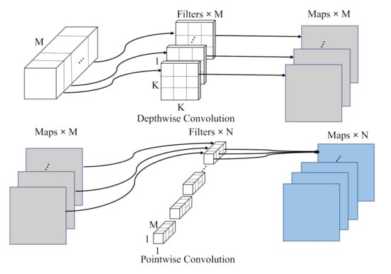
Figure 2.
The structure of depthwise separable convolution.
2.4. Data Pre-Processing
First, due to the limitations of hardware devices, large remote sensing images cannot be directly imported into the classification network. In this paper, we cut the remote sensing images into non-overlapping patches for model training. Second, we use a data-balancing strategy. If the background of the image is too high, we will discard the image. On the contrary, we do not do anything with it. Finally, as the depth of the network increases, the convergence of the network becomes difficult and the training speed becomes very slow. In order to improve the accuracy of the network and training efficiency, it is necessary to standardize the input images. The distribution of the input image is standardized to a normal distribution with a mean of 0 and variance of 1. The formulas are as follows:
where c, w, and h are the channel, width, and height of the input images, is the mean of the input image, and is the variance of the input image. I and are the input images and the result of its normalization, respectively.
2.5. Model Structure
Over the past few years, deep learning methods, represented by semantic segmentation, have become the state-of-the-art pixel level classification algorithms in the field of remote sensing image processing. In the remote sensing images, due to the different sizes of lakes and the influence of noise such as shadows and snow, the standard convolution has great limitations in its application and cannot classify the central pixels correctly. As shown in Figure 3, the model proposed in the paper uses the modified ResNet-101 as an encoder to extract deep semantic features and sends the output feature maps in four ways to a multi-scale densely connected feature extractor module for extracting features at different scales. Finally, by combining it with the shallow features of the encoder, we obtain the predicted label maps of lake water bodies.
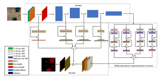
Figure 3.
The structure of the multi-scale lake water extraction network. It consists of three main parts: an encoder, a multi-scale densely connected feature extractor, and a decoder.
2.5.1. Residual Learning Module
The results of the research show that the more the layers of the neural network, the better the fit to the data is [30]. As the depth increases, the performance of the network does not improve, most likely due to the disappearance of the gradient during the back propagation between layers. The gradient is so small that it cannot update the layer parameters. This problem can be solved by a residual learning module of ResNet. A typical residual learning module is shown in Figure 4 (left). The residual learning module bypasses the inputs and outputs of the convolutional layer so that those small gradients can be bypassed to compensate for the vanishing gradients. In the encoder stage, as shown in Figure 4 (mid), due to the difference in size and number of channels between the input and output feature maps, the traditional residual structure cannot be used directly. Therefore, it is necessary to adjust the size of the input feature maps in the bypass using a convolution for channel adjustment or down-sampling.
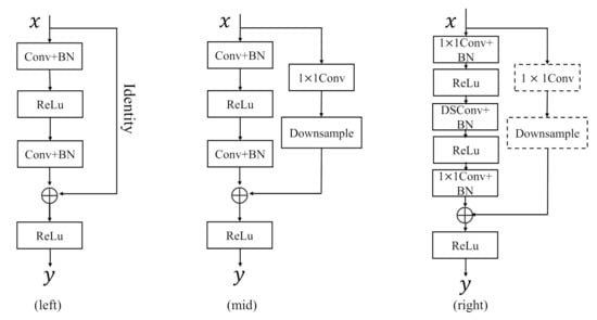
Figure 4.
The structure of the residual learning module. (left) is a typical residual learning module, (mid) is a residual learning module commonly used in the encoder stage, and (right) is the residual learning module used in our model.
As the depth of the network gets deeper, the number of parameters in the model will increase, making it easy to overfit our dataset. Inspired by Xception [31] and MobileNet [32], we replace the convolution in the residual learning module with a depthwise separable convolution to reduce the number of parameters in the model. For the example in Figure 4 (right), the residual learning module can be defined as:
where x and y are the input and output of the residual learning module, respectively, and (i ∈ N) represents the parameter settings of the convolutional layer with a kernel size of . represents batch normalization (BN) [38], and its role is to convert the input distribution into a standard normal distribution with a mean of 0 and variance of 1 to accelerate the convergence of the network. represents the activation function. In this paper, we use the rectified linear unit (ReLU) [39] as the activation function, which has become the mainstream function in the field of the semantic segmentation of remote sensing images. Its formula is as follows:
2.5.2. Multi-Scale Densely Connected Feature Extractor
The difficulty of lake water body extraction lies in the existence of noise in remote sensing images, which have similar features as water bodies, and the existence of differences in the size of lakes. In order to improve the extraction accuracy of lake water bodies, the multi-scale high level semantic information of lakes needs to be fully extracted and effectively encoded. DeepLab V3+ [25] proposes atrous spatial pyramid pooling module (ASPP) to capture the contextual information of feature maps at multiple scales by parallel sampling at different dilated rates. However, the extraction accuracy of small water bodies and the ability of suppressing noise are still not high. This paper improves this based on this idea and designs a multi-scale densely connected feature extractor.
The use of dilated convolution can lead to sparse convolutional kernels and a large amount of computational information will be lost. To solve this problem, denser computation is needed by increasing the expansion factor. First, the convolution is used for dimensionality adjustment to reduce the number of parameters. Then, we use a gradual expansion factor to make the receptive field larger and denser. Prior to each dilated convolution, the feature map is channeled to the previous layer to obtain more detailed contextual information, in order to improve the accuracy of water bodies’ extraction in small lakes. The most significant aspect of the multi-scale densely connected feature extraction module is to extract and fuse high level semantic information at different scales, which is very effective for pixel level classification, thus solving the problem of small water bodies’ extraction and noise interference.
3. Experiment
3.1. Implementation Details
In this paper, our experiment was based on Python3.6 and the open source deep learning framework PyTorch [40]. The GPU was NVIDIA 2070 SUPER, having 8GB of RAM and using cuDNN 10.0 for acceleration. The CPU was an AMD Ryzen 5 3600, with a frequency of 3.6GHz. Our model was not pre-trained initialized, and all initial weights of the convolutional layers were obtained from Kaiming initialization [41]. We shuffled all the images before the start of each epoch to improve the generalization of the model and set the batch sizes to 8. In this experiment, the cross-entropy loss [42] was calculated by predicted label maps and GT labels. Its formula is as follows:
where and are the true probability distribution and the predicted probability distribution, respectively. To minimize the cross-entropy loss, the Adam [43] optimizer was used to update the parameters of the model and set the weight decay to 0.001 to prevent overfitting. The initial learning rate was set to 0.001 with the learning rate decline strategy, which can be represented as Formula (9). represents the initial learning rate. indicates the times to train the full sample of the training set. The reason for using a learning rate decay strategy is that a larger learning rate at a later stage of training will prevent the model from converging to a minimum value, thus not providing optimal results. Our model achieved optimal performance after 70 epochs.
3.2. Dataset
In this paper, we create a new visible-spectrum Google Earth remote sensing images of lake water bodies dataset captured on the Tibetan Plateau, which consists of RGB images. The images were divided into non-overlapping patches, to obtain 6774 images sized 256 × 256 with a DPI of 96 and a bit depth of 24. In this dataset, only lakes (excluding rivers, reservoirs, ponds, etc.) were positively annotated, all of which were labeled using labelme. We randomly selected 6164 images for training and the remaining 610 images for testing. We did not set the validation set due to the limitations of our dataset.
The lakes on the Tibetan Plateau can be typologically divided into salt and freshwater lakes. The shores of salt lakes are accompanied by salt belts, which present a complex texture. Freshwater lakes are white, light blue, dark blue, and black in spectral features. Black lakes have similar features to the shadows of mountains and clouds, while white lakes have similar features to snow. In terms of state, there are frozen, semi-frozen, and non-frozen lakes. The study area and its overview are shown in Figure 5.
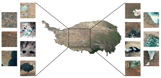
Figure 5.
The study area of lake water bodies’ extraction.
Data augmentation is one of the techniques commonly used in deep learning, mainly used to generate new samples to increase the training dataset when the training sample is small. In this paper, we use the most common methods of flipping (up and down, left and right) and rotating (, ) for all the training samples before each training epoch, and the results of data augmentation are shown in Figure 6.
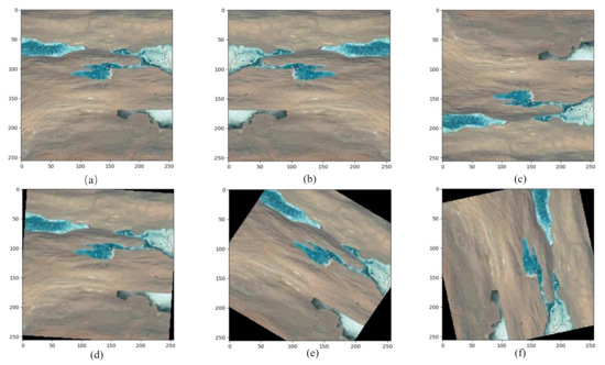
Figure 6.
Examples of data augmentation. (a) is the original image; (b) is flipping the original image left and right; and (c) is flipping the original image up and down. (d–f) is rotating the original image at any angle of (, ).
3.3. Results
To assess the performance of our proposed model, we used the five evaluation metrics, which are overall accuracy (OA), recall, the mean intersection over union (MIoU), the true water rate (TWR) [10], and the false water rate (FWR) [10]. OA is the ratio of the correctly classified pixel numbers to the total pixel numbers in the test dataset. Recall is the ratio of the number of pixels correctly predicted to be a lake to all the number of pixels for the lake. MIoU is the average of the ratio of the number of correctly classified pixels to the number of ground reference pixels and the number of pixels detected in the corresponding category. TWR is the ratio of the number of properly classified water pixels and the number of labeled water pixels. FWR is the ratio of the number of misclassified water pixels and the number of labeled water pixels. The formulas of these indicators are as follows:
3.3.1. Comparison of Overall Performance among Different CNNs
To analyze the performance of the classification algorithms proposed in this paper, Unet, MWEN, PSPNet, and DeepLab V3+ were used to perform the comparisons. After obtaining the optimal model, the test images were predicted. The metrics of these models are shown in Table 1. Our model improves by 0.43% relative to DeepLab V3+, one of the best models for image segmentation. For the Unet model, the depth is not sufficient to extract deep semantic features at the encoding stage, resulting in poor accuracy. Although, the OA improvement is not much, there are significant improvements in small lake water body extraction and noise interference suppression. We also applied depthwise separable convolution in our model to get higher accuracy with fewer parameters. The efficiency of the training model is influenced by many factors, and the depthwise separable convolution theoretically reduces the computational effort. Due to its poor optimization by cuDNN, the training time is not significantly reduced, as shown in Table 2 for a comparison of the number of model parameters and training time.

Table 1.
The metrics of the CNN models in the testing phase. MSLWENet, multi-scale lake water extraction network; MIoU, mean intersection over union; TWR, true water rate; FWR, false water rate.

Table 2.
Comparing CNN models in the number of parameters and training time.
3.3.2. Performance Comparison for Small Lakes’ Identification
With the gradual improvement in the resolution of remote sensing satellites, an increasing amount of detail in remote sensing images becomes visible. Small lakes are an important challenge for lake water extraction. We used the strategy introduced in Section 2.5.2 to improve the extraction accuracy of small lakes. The visualization results are shown in Figure 7, and the quantitative results are shown in Table 3.
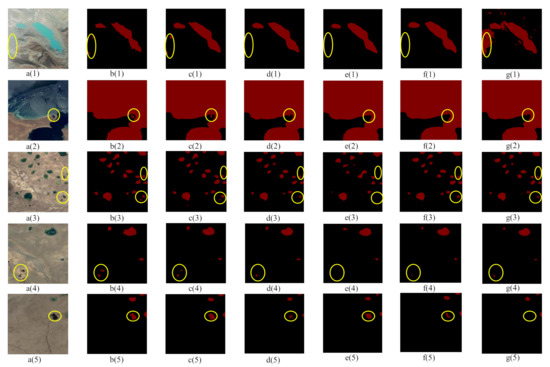
Figure 7.
Performance comparison of different models for small lake water extraction. (a(1)–a(5)) are the raw images in the test set; (b(1)–b(5)) are the ground truths to which the raw images correspond; (c(1)–c(5)), (d(1)–d(5)), (e(1)–e(5)), (f(1)–f(5)), and (g(1)–g(5)) are the extracted results of MSLWENet, DeepLab V3+, PSPNet, MWEN, and Unet, respectively.

Table 3.
The metrics of the CNN models on the images in Figure 7.
As we see, the input image contains a large number of small water bodies of the lakes that are very close to each other, shadows, and tiny boundaries. These factors have a significant impact on the performance of the model for small lake extractions. As shown in Figure 7, the network we propose in this paper is basically able to extract small lakes from remote sensing images quite well, but it is still lacking in the accuracy of the boundaries, while other networks give some incorrect segmentations for the small lakes. In Figure 7g(1), it is possible that the features extracted by Unet are not sufficient and thus cannot handle the complex regions well enough, resulting in a large number of misclassifications. As shown in Table 3, MSLWENet improves by 0.13% on OA and 1.47% on TWR relative to DeepLab V3+. It shows that our model is able to extract small water bodies well.
3.3.3. Performance Comparison of Small Interclass Variance Regions
In remote sensing images, shadows, snow, and other disturbances have similar spectral characteristics to lakes, which have a significant impact on lake water body extraction. In order to compare the robustness of these networks to noise interference, the visualization results are shown in Figure 8 and the quantitative results are shown in Table 4.
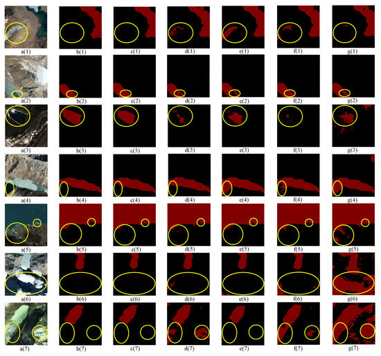
Figure 8.
Performance comparison of different models for lake water extraction from small interclass variance regions. (a(1)–a(7)) are the raw images in the test set; (b(1)–b(7)) are the ground truths to which the raw images correspond; (c(1)–c(7)), (d(1)–d(7)), (e(1)–e(7)), (f(1)–f(7)), and (g(1)–g(7)) are the extracted results of MSLWENet, DeepLab V3+, PSPNet, MWEN, and Unet, respectively.

Table 4.
The metrics of the CNN models on the images in Figure 8.
In Figure 8 (Rows 1, 6–7), frozen lakes and snow are very similar in spectral features, and shadows are also one of the major factors in the accuracy of lake water body extraction, which can easily lead to misclassification. DeepLab V3+, PSPNet, MWEN, and Unet all more or less mistake snow for frozen lakes. In Figure 8e(7), PSPNet is able to suppress the noise interference well, yet it does not fully extract the detailed boundaries of the lake water bodies. An incompletely frozen lake appears in Figure 8 (Row 2), where DeepLab V3+ and MWEN produce better results relative to PSPNet and Unet, mainly in the presence of less noise within the water bodies. In Figure 8g(5), Unet identifies the text on the image as a lake. In Figure 8 (Row 3), the lake is black in the spectrum, while in Figure 8 (Row 4), there are black shadows. Our proposed MSLWENet is able to get as accurate segmentation results as possible while discriminating the shadows as interfering factors, while other models can only do one of the two. For all input images, Unet produces the worst segmentation results. As shown in Table 4, PSPNet performs better than DeepLab V3+ in the region of small inter-class variance, but MSLWENet has a greater improvement over PSPNet.
3.3.4. Performance Comparison of Large Intraclass Variance Regions
In the Google remote sensing images, due to the different shooting seasons, the lakes show a large intra-class variance, even if they are all frozen lakes. They are very different in texture and spectral features; therefore, it is an important challenge to correctly segment the lakes with different features. The visualization results are shown in Figure 9, and the quantitative results are shown in Table 5.
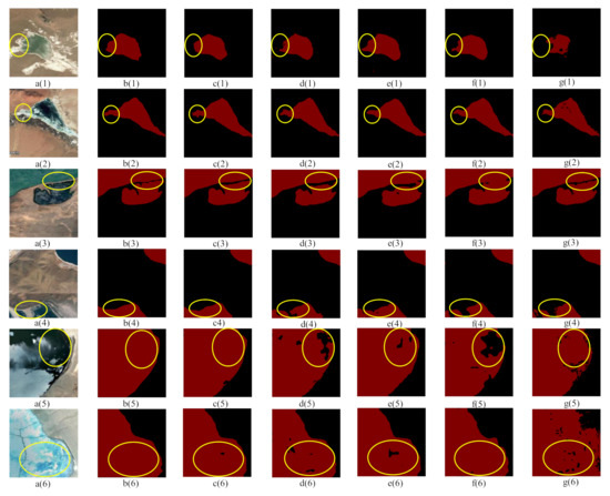
Figure 9.
Performance comparison of different models for lake water extraction from large intraclass variance regions. (a(1)–a(6)) are the raw images in the test set; (b(1)–b(6)) are the ground truths to which the raw images correspond; (c(1)–c(6)), (d(1)–d(6)), (e(1)–e(6)), (f(1)–f(6)), and (g(1)–g(6)) are the extracted results of MSLWENet, DeepLab V3+, PSPNet, MWEN, and Unet, respectively.

Table 5.
The metrics of the CNN models on the images in Figure 9.
As shown in Figure 9 (Rows 1–3), all models basically do a good job at segmenting the lake water bodies. However, there are still differences in some of the details marked by the yellow circles on the images. For some lakes with complex textures in Figure 9 (Rows 4–6), DeepLab V3+, PSPNet, and MWEN can segment the lake water bodies and land well, but there is much noise on the surface of the lakes, while the performance of Unet is still not good enough. Our proposed model is able to extract different types of lake water bodies completely, with robustness and generalization capabilities. As in Section 3.3.3, PSPNet has better performance relative to DeepLab V3+; however, MSLWENet improves by 1.24% on MIoU relative to PSPNet.
3.3.5. Performance Comparison of Different Encoders and Decoders
In this subsection, we focus on the impact of different encoders and decoders on the performance during the presentation of our model. The performance comparisons are shown in Table 6. Firstly, in order to reduce the parameters and training time of the model, we used VGG-16 as the backbone network in the encoder part and the same decoder as our proposed model. Although it reduces the trainable parameters and training time of the model, it only improves the performance by 1.25% compared to Unet, which is not satisfactory. This may be due to the inability of VGG-16 to extract rich semantic information for segmentation. Secondly, we used ResNet-101 as the backbone extraction network, operated with layer-by-layer up-sampling in the decoder part and element-wise summing with different feature layers in the encoder. Compared to DeepLab V3+, it improves performance by 0.07%, but the training time is significantly longer. Finally, we used ResNet-101 with depthwise separable convolution as the backbone network to extract features while reducing the parameters of the model. In the decoder part, the label prediction map is obtained by using the channel connection method and reusing features from different layers of the encoder. Compared to DeepLab V3+, the overall accuracy is improved by 0.43% without increasing the training time, while reducing the number of parameters. The visualization results are shown in Figure 10.

Table 6.
Performance comparison of different encoders and decoders in Figure 10.
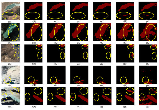
Figure 10.
Performance comparison of different encoders and decoders. (a(1)–a(5)) are the raw images in the test set; (b(1)–b(5)) are the ground truths to which the raw images correspond; (c(1)–c(5)), (d(1)–d(5)), (e(1)–e(5)), (f(1)–f(5)), and (g(1)–g(5)) are the extracted results of MSLWENet, DeepLab V3+, ResNet-Sum, VGG-Concat, and Unet, respectively.
4. Discussion
With the improvement in the resolution of remote sensing images, the methods of water extraction are changing, such as thresholding, machine learning, and deep learning. The Tibetan Plateau is the highest, most numerous and largest lake region on Earth and one of the two most densely distributed lake regions in China.
In this paper, our proposed method named MSLWENet achieves state-of-the-art performance on the lake dataset than DeepLab V3+, PSPNet, MWEN, and Unet. In Section 3, the performance of the model is evaluated by five evaluation metrics and visualization results. In particular, our method achieves an overall accuracy of 98.53%, an improvement of 0.43% over DeepLab V3+. In small lake water extraction, OA is not much improved due to the large portion of background in the image, but TWR is improved by 1.47% compared to DeepLab V3+. This result shows that the proposed model is capable of extracting small lakes. In the large intra-class variance and small inter-class variance regions, PSPNet has better performance than DeepLab V3+. However, MSLWENet has improved performance over other CNN models, which means it can suppress noise better. The results are mainly from the multi-scale densely connected feature extraction module, which is a good solution to the problem of information loss caused by a large dilated rate and a too small dilated rate to correctly identify noise. We fully utilize spatial and channel dimensional features to better capture the multi-scale relationship between pixels, resulting in the better feature extraction capability and segmentation performance of our model. In Section 3.3.5, MSLWENet improves the OA by 1.16% compared to VGG-Concat. The result shows that using VGG-16 as the backbone extraction network does not extract enough semantic features for segmentation and may be an argument for the poor performance of Unet. Furthermore, MSLWENet improves the OA by 0.36% compared to ResNet-Sum. The result shows that the operation with the channel connection has a greater improvement in performance than element-by-element addition, which may be related to its ability to retain more information during up-sampling.
The segmentation performance of these convolutional neural networks may be related to their own structure and dataset complexity. For relatively simple datasets, overly complex neural network models are prone to overfitting. FCN and Unet will be able to achieve better performance. On the other hand, the datasets in this paper have complex texture and spectral features, so more complex models are required for feature extraction, such as DeepLab V3+, PSPNet, and other networks. However, since our dataset is relatively small, we apply depthwise separable convolution in our model to drastically reduce the number of trainable parameters to effectively suppress overfitting.
5. Conclusions
In this paper, a new MSLWENet model for remote sensing image semantic segmentation based on convolutional neural networks is proposed. The adopted structure consists of an encoder, a multi-scale dense connect module, and a decoder. For feature extraction, a modified ResNet-101 is used as the feature extractor, where the residual structure is capable of extracting a large number of useful semantic features without causing degradation of the model. Dilated convolution is necessary due to lakes’ scale features, but excessive dilated rates can lead to the loss of useful information and incomplete segmentation of small lakes, so we use progressively larger dilated rates and connect channels at different layers of dilated convolution to preserve as much information as possible. In the training process of the model, we use data augmentation processing, which can avoid overfitting of the network and improve the generalization of the network. Compared to existing models, the method achieves the highest OA, recall, MIoU, and TWR and the lowest FWR, while the integrity of the segmented lake is significantly better than other methods.
Although our method achieves good segmentation results on this dataset, there are still many shortcomings, which will guide our future research directions. Due to the relatively small size of our dataset, it is easy to overfit the model. On the one hand, we need to enrich our dataset, and on the other hand, pre-training on ImageNet and fine-tuning on our dataset would be a better solution. Finally, due to the rich surface texture of lakes, segmentation is prone to noise, so some morphological treatments, such as conditional random fields and morphological filtering, will be applied to optimize the segmentation results.
Author Contributions
Methodology, X.G.; resources, G.Z.; data curation, X.G.; writing, original draft preparation, X.G.; writing, review and editing, Z.W.; supervision, Z.W.; project administration, Y.Z.; funding acquisition, Z.W. All authors read and agreed to the published version of the manuscript.
Funding
This research was funded by the National Natural Science Foundation of China (Grant No. 61201421), the National cryosphere desert data center (Grant No. E01Z7902), and the Capability improvement project for cryosphere desert data center of the Chinese Academy of Sciences (Grant No. Y9298302).
Acknowledgments
We would like to thank all the people who helped and supported our research, especially Minzhe Xu, Yikun Ma, and Zhongxin Cheng and the staff at CAS.
Conflicts of Interest
The authors declare no conflict of interest.
References
- Downing, J.; Prairie, Y.; Cole, J.; Duarte, C.; Tranvik, L.; Striegl, R.G.; McDowell, W.; Kortelainen, P.; Caraco, N.; Melack, J.; et al. The global abundance and size distribution of lakes, ponds, and impoundments. Limnol. Oceanogr. 2006, 51, 2388–2397. [Google Scholar] [CrossRef]
- Tranvik, L.; Downing, J.; Cotner, J.; Loiselle, S.; Striegl, R.; Ballatore, T.; Dillon, P.; Knoll, L.; Kutser, T.; Larsen, S.; et al. Lakes and reservoirs as regulators of carbon cycling and climate. Limnol. Oceanogr. 2009, 54, 2298–2314. [Google Scholar] [CrossRef]
- Singh, J.; Upadhyay, S.; Pathak, R.; Gupta, V. Accumulation of heavy metals in soil and paddy crop (Oryza sativa), irrigated with water of Ramgarh Lake, Gorakhpur, UP, India. Toxicol. Environ. Chem. 2011, 93, 462–473. [Google Scholar] [CrossRef]
- Qin, B.; Zhu, G.; Gao, G.; Zhang, Y.; Li, W.; Paerl, H.W.; Carmichael, W.W. A drinking water crisis in Lake Taihu, China: Linkage to climatic variability and lake management. Environ. Manag. 2010, 45, 105–112. [Google Scholar] [CrossRef]
- Hofmann, H.; Lorke, A.; Peeters, F. The relative importance of wind and ship waves in the littoral zone of a large lake. Limnol. Oceanogr. 2008, 53, 368–380. [Google Scholar] [CrossRef]
- Li, R.; Liu, W.; Yang, L.; Sun, S.; Hu, W.; Zhang, F.; Li, W. DeepUNet: A Deep Fully Convolutional Network for Pixel-Level Sea-Land Segmentation. IEEE J. Sel. Top. Appl. Earth Obs. Remote Sens. 2018, 11, 3954–3962. [Google Scholar] [CrossRef]
- Cheng, D.; Meng, G.; Xiang, S.; Pan, C. Fusionnet: Edge aware deep convolutional networks for semantic segmentation of remote sensing harbor images. IEEE J. Sel. Top. Appl. Earth Obs. Remote Sens. 2017, 10, 5769–5783. [Google Scholar] [CrossRef]
- Feyisa, G.L.; Meilby, H.; Fensholt, R.; Proud, S.R. Automated Water Extraction Index: A new technique for surface water mapping using Landsat imagery. Remote Sens. Environ. 2014, 140, 23–35. [Google Scholar] [CrossRef]
- Zhang, F.; Li, J.; Zhang, B.; Shen, Q.; Ye, H.; Wang, S.; Lu, Z. A simple automated dynamic threshold extraction method for the classification of large water bodies from landsat-8 OLI water index images. Int. J. Remote Sens. 2018, 39, 3429–3451. [Google Scholar] [CrossRef]
- Zhang, Y.; Liu, X.; Zhang, Y.; Ling, X.; Huang, X. Automatic and Unsupervised Water Body Extraction Based on Spectral-Spatial Features Using GF-1 Satellite Imagery. IEEE Geosci. Remote Sens. Lett. 2018, 16, 927–931. [Google Scholar] [CrossRef]
- Huang, X.; Xie, C.; Fang, X.; Zhang, L. Combining pixel-and object-based machine learning for identification of water-body types from urban high-resolution remote-sensing imagery. IEEE J. Sel. Top. Appl. Earth Obs. Remote Sens. 2015, 8, 2097–2110. [Google Scholar] [CrossRef]
- Miao, Z.; Fu, K.; Sun, H.; Sun, X.; Yan, M. Automatic water-body segmentation from high-resolution satellite images via deep networks. IEEE Geosci. Remote Sens. Lett. 2018, 15, 602–606. [Google Scholar] [CrossRef]
- Chen, Y.; Fan, R.; Yang, X.; Wang, J.; Latif, A. Extraction of urban water bodies from high-resolution remote-sensing imagery using deep learning. Water 2018, 10, 585. [Google Scholar] [CrossRef]
- Guo, H.; He, G.; Jiang, W.; Yin, R.; Yan, L.; Leng, W. A Multi-Scale Water Extraction Convolutional Neural Network (MWEN) Method for GaoFen-1 Remote Sensing Images. ISPRS Int. J. Geo-Inf. 2020, 9, 189. [Google Scholar] [CrossRef]
- Jiang, H.; Feng, M.; Zhu, Y.; Lu, N.; Huang, J.; Xiao, T. An automated method for extracting rivers and lakes from Landsat imagery. Remote Sens. 2014, 6, 5067–5089. [Google Scholar] [CrossRef]
- Mondejar, J.P.; Tongco, A.F. Near infrared band of Landsat 8 as water index: A case study around Cordova and Lapu-Lapu City, Cebu, Philippines. Sustain. Environ. Res. 2019, 29, 16. [Google Scholar] [CrossRef]
- McFeeters, S.K. The use of the Normalized Difference Water Index (NDWI) in the delineation of open water features. Int. J. Remote Sens. 1996, 17, 1425–1432. [Google Scholar] [CrossRef]
- Xu, H. Modification of normalised difference water index (NDWI) to enhance open water features in remotely sensed imagery. Int. J. Remote Sens. 2006, 27, 3025–3033. [Google Scholar] [CrossRef]
- Chen, C.; Chen, J.; Li, X.; Zhang, Q.; Zheng, S. Study on water body information extraction from high resolution remote sensing image based on object-oriented method. Yellow River 2013, 35, 68–70. [Google Scholar]
- Cortes, C.; Vapnik, V. Support-vector networks. Mach. Learn. 1995, 20, 273–297. [Google Scholar] [CrossRef]
- Breiman, L. Random forests. Mach. Learn. 2001, 45, 5–32. [Google Scholar] [CrossRef]
- Long, J.; Shelhamer, E.; Darrell, T. Fully convolutional networks for semantic segmentation. In Proceedings of the IEEE Conference on Computer Vision and Pattern Recognition, Boston, MA, USA, 7–12 June 2015; pp. 3431–3440. [Google Scholar]
- Badrinarayanan, V.; Kendall, A.; Cipolla, R. Segnet: A deep convolutional encoder-decoder architecture for image segmentation. IEEE Trans. Pattern Anal. Mach. Intell. 2017, 39, 2481–2495. [Google Scholar] [CrossRef]
- Ronneberger, O.; Fischer, P.; Brox, T. U-net: Convolutional networks for biomedical image segmentation. In Lecture Notes in Computer Science, Proceedings of the International Conference on Medical Image Computing and Computer-Assisted Intervention, Munich, Germany, 5–9 October 2015; Springer: Cham, Switzerland, 2015; pp. 234–241. [Google Scholar]
- Chen, L.C.; Zhu, Y.; Papandreou, G.; Schroff, F.; Adam, H. Encoder-decoder with atrous separable convolution for semantic image segmentation. In Proceedings of the European Conference on Computer Vision (ECCV), Munich, Germany, 8–14 September 2018; pp. 801–818. [Google Scholar]
- Girshick, R.; Donahue, J.; Darrell, T.; Malik, J. Rich feature hierarchies for accurate object detection and semantic segmentation. In Proceedings of the IEEE Conference on Computer Vision and Pattern Recognition, Columbus, OH, USA, 24–27 June 2014; pp. 580–587. [Google Scholar]
- Ren, S.; He, K.; Girshick, R.; Sun, J. Faster r-cnn: Towards real-time object detection with region proposal networks. In Proceedings of the Advances in Neural Information Processing Systems, Montreal, QC, Canada, 7–12 December 2015; pp. 91–99. [Google Scholar]
- Krizhevsky, A.; Sutskever, I.; Hinton, G.E. Imagenet classification with deep convolutional neural networks. In Proceedings of the Advances in Neural Information Processing Systems, Lake Tahoe, NV, USA, 3–8 December 2012; pp. 1097–1105. [Google Scholar]
- Simonyan, K.; Zisserman, A. Very Deep Convolutional Networks for Large-Scale Image Recognition. arXiv 2014, arXiv:1409.1556. [Google Scholar]
- He, K.; Zhang, X.; Ren, S.; Sun, J. Deep residual learning for image recognition. In Proceedings of the IEEE Conference on Computer Vision and Pattern Recognition, Las Vegas, NV, USA, 27–30 June 2016; pp. 770–778. [Google Scholar]
- Chollet, F. Xception: Deep learning with depthwise separable convolutions. In Proceedings of the IEEE Conference on Computer Vision and Pattern Recognition, Honolulu, HI, USA, 21–26 July 2017; pp. 1251–1258. [Google Scholar]
- Howard, A.G.; Zhu, M.; Chen, B.; Kalenichenko, D.; Wang, W.; Weyand, T.; Andreetto, M.; Adam, H. Mobilenets: Efficient convolutional neural networks for mobile vision applications. arXiv 2017, arXiv:1704.04861. [Google Scholar]
- Leung, H.; Haykin, S. The complex backpropagation algorithm. IEEE Trans. Signal Process. 1991, 39, 2101–2104. [Google Scholar] [CrossRef]
- Holschneider, M.; Kronland-Martinet, R.; Morlet, J.; Tchamitchian, P. A real-time algorithm for signal analysis with the help of the wavelet transform. In Wavelets; Springer: Berlin/Heidelberg, Germany, 1990; pp. 286–297. [Google Scholar]
- Chen, L.C.; Papandreou, G.; Schroff, F.; Adam, H. Rethinking atrous convolution for semantic image segmentation. arXiv 2017, arXiv:1706.05587. [Google Scholar]
- Chen, L.C.; Papandreou, G.; Kokkinos, I.; Murphy, K.; Yuille, A.L. Semantic image segmentation with deep convolutional nets and fully connected crfs. arXiv 2014, arXiv:1412.7062. [Google Scholar]
- Sifre, L.; Mallat, S. Rigid-motion scattering for texture classification. arXiv 2014, arXiv:1403.1687. [Google Scholar]
- Ioffe, S.; Szegedy, C. Batch normalization: Accelerating deep network training by reducing internal covariate shift. arXiv 2015, arXiv:1502.03167. [Google Scholar]
- Nair, V.; Hinton, G.E. Rectified linear units improve restricted boltzmann machines. In Proceedings of the ICML, Haifa, Israel, 21–24 June 2010; pp. 770–778. [Google Scholar]
- Paszke, A.; Gross, S.; Massa, F.; Lerer, A.; Bradbury, J.; Chanan, G.; Killeen, T.; Lin, Z.; Gimelshein, N.; Antiga, L.; et al. Pytorch: An imperative style, high-performance deep learning library. In Proceedings of the Advances in Neural Information Processing Systems, Vancouver, BC, Canada, 8–14 December 2019; pp. 8026–8037. [Google Scholar]
- He, K.; Zhang, X.; Ren, S.; Sun, J. Delving deep into rectifiers: Surpassing human-level performance on imagenet classification. In Proceedings of the IEEE International Conference on Computer Vision, Santiago, Chile, 11–18 December 2015; pp. 1026–1034. [Google Scholar]
- De Boer, P.T.; Kroese, D.P.; Mannor, S.; Rubinstein, R.Y. A tutorial on the cross-entropy method. Ann. Oper. Res. 2005, 134, 19–67. [Google Scholar] [CrossRef]
- Kingma, D.P.; Ba, J. Adam: A method for stochastic optimization. arXiv 2014, arXiv:1412.6980. [Google Scholar]
Publisher’s Note: MDPI stays neutral with regard to jurisdictional claims in published maps and institutional affiliations. |
© 2020 by the authors. Licensee MDPI, Basel, Switzerland. This article is an open access article distributed under the terms and conditions of the Creative Commons Attribution (CC BY) license (http://creativecommons.org/licenses/by/4.0/).