Article

Lake Phenology of Freeze-Thaw Cycles Using Random Forest: A Case Study of Qinghai Lake

1
Key Laboratory of Remote Sensing of Gansu Province, Heihe Remote Sensing Experimental Research Station, Northwest Institute of Eco-Environment and Resources, Chinese Academy of Sciences, Lanzhou 730000, China
2
University of Chinese Academy of Sciences, Beijing 100049, China
3
Key Laboratory of Watershed Geographic Sciences, Nanjing Institute of Geography and Limnology, Chinese Academy of Sciences, 73 East Beijing Road, Nanjing 210008, China
4
College of Urban and Environmental Sciences, Northwest University, Xi’an 710127, China
5
Key Laboratory of Western China’s Environmental Systems, Ministry of Education, Lanzhou University, Lanzhou 730000, China
*
Author to whom correspondence should be addressed.
Remote Sens. 2020, 12(24), 4098; https://doi.org/10.3390/rs12244098
Submission received: 17 October 2020 / Revised: 11 December 2020 / Accepted: 13 December 2020 / Published: 15 December 2020
(This article belongs to the Special Issue Satellite Hydrological Data Products and Their Applications)

Abstract

:
Lake phenology is essential for understanding the lake freeze-thaw cycle effects on terrestrial hydrological processes. The Qinghai-Tibetan Plateau (QTP) has the most extensive ice reserve outside of the Arctic and Antarctic poles and is a sensitive indicator of global climate changes. Qinghai Lake, the largest lake in the QTP, plays a critical role in climate change. The freeze-thaw cycles of lakes were studied using daily Moderate Resolution Imaging Spectroradiometer (MODIS) data ranging from 2000–2018 in the Google Earth Engine (GEE) platform. Surface water/ice area, coverage, critical dates, surface water, and ice cover duration were extracted. Random forest (RF) was applied with a classifier accuracy of 0.9965 and a validation accuracy of 0.8072. Compared with six common water indexes (tasseled cap wetness (TCW), normalized difference water index (NDWI), modified normalized difference water index (MNDWI), automated water extraction index (AWEI), water index 2015 (WI2015) and multiband water index (MBWI)) and ice threshold value methods, the critical freeze-up start (FUS), freeze-up end (FUE), break-up start (BUS), and break-up end (BUE) dates were extracted by RF and validated by visual interpretation. The results showed an R2 of 0.99, RMSE of 3.81 days, FUS and BUS overestimations of 2.50 days, and FUE and BUE underestimations of 0.85 days. RF performed well for lake freeze-thaw cycles. From 2000 to 2018, the FUS and FUE dates were delayed by 11.21 and 8.21 days, respectively, and the BUS and BUE dates were 8.59 and 1.26 days early, respectively. Two novel key indicators, namely date of the first negative land surface temperature (DFNLST) and date of the first positive land surface temperature (DFPLST), were proposed to comprehensively delineate lake phenology: DFNLST was approximately 37 days before FUS, and DFPLST was approximately 20 days before BUS, revealing that the first negative and first positive land surface temperatures occur increasingly earlier.

Graphical Abstract

1. Introduction

Lakes (surface area of at least 10 ha) occupy 1.8% of the global land surface area [1] and can impact both local weather and climate [2,3]. In terms of global climate change, lake phenology events, such as critical surface water freeze-up dates, lake ice break-up dates, ice cover duration, and land surface temperature (LST), could serve as useful indicators for monitoring climate change [4]. The Qinghai-Tibetan Plateau (QTP) has both the largest number of lakes (1055, 39.2%) and the largest total lake area (41,831.7 km2, 51.4%) in China [5]. As global warming continues or even accelerates, lake responses may resonate far beyond the isolated QTP, changing the water supplies for billions of people and altering the atmospheric circulation over half of the planet [6]. In addition, impacts on lake ice cover and formation could impact socio-economic elements such as icy roads, transportation, cultural recreation, and tourism [7]. Many lakes with large areas have sensitive responses to climate change and play essential roles in climate change [8]. Lakes influence the climate by changing underlying surface conditions through differences in lake surface water and ice areas or physical status [9]. Since these lakes are located on the high-altitude QTP, which has a cold climate, these lakes are less disturbed by human activities. Therefore, variations and changes essentially reflect natural environmental changes due to climate change [10]. Earlier lake phenology research dates back to the 1860s, which included research on the statistical relationships among freeze-up start (FUS) dates, freeze-up end (FUE) dates, break-up start (BUS) dates and break-up end (BUE) dates of lakes and air temperature in Finland [11]. These dates control the ice season and are strongly determined by the temperature. Additionally, the thermal structure and water-ice heat transfer in a shallow ice-covered thermokarst lake in the central QTP was explained [12].
Lake ice and surface water data collection depend mainly on classic methods, including aerial surveys, field observations, and hydrological observations. However, these observational types are often influenced by regional conditions and untraversed sites. The sparse collection of in situ data and complete long-term metadata are difficult to obtain using these methods [13]. Remote sensing images at various geospatial and temporal resolutions could compensate for classic observation shortcomings. Advanced very high-resolution radiometer data were used to extract the dates of freeze-thaw cycle lakes in Canada from 1985–2004 by setting a reflectance threshold value. The results showed that remote sensing data are highly consistent with ground observation records [14]. Moderate Resolution Imaging Spectroradiometer (MODIS) eight-day composite data were used to analyze the variabilities in freeze-thaw cycle dates of lake ice for 59 large lakes on the QTP for the 2001–2010 period [15]. Remote sensing data have advantages in terms of high temporal and spatial resolutions and rich multi-spectral information. However, long-term data volumes are large, which results in only a few images for each year from long-term series. All images cover each year, and adequate remote sensing data usage is limited. Simultaneously, remote sensing images are affected by the cloud. The presence of clouds hinders the quantitative extraction of surface for such purposes as classification and monitoring of land-use and land-cover changes [16,17]. Therefore, it remains challenging to identify the water and ice with cloud-contamination images over a mountain region. A cloud filtering method was applied to extract the upper tropospheric humidity measurements [18].
Remote sensing methods for lake and river ice and surface water have received widespread research focus, especially ice phenology [19]. Ice threshold value methods have been widely used in lake ice studies, and the ice phenology date’s errors were within five days [20]. A new dynamic threshold technique was applied to identify and map lake ice cover in Geostationary Operational Environmental Satellite 13 images [21]. The QTP lake area was identified using an automated waterbody interpretation method for the 1980s to 2015 period [22].
There are many water indexes to quantifying the characteristics of water using remote sensing. Including tasseled cap wetness (TCW) [23], water index and modified fuzzy clustering method (WIMFCM) [24], normalized difference water index (NDWI) [25], modified normalized difference water index (MNDWI) [26], multiband water index (MBWI) [27], water index 2015 (WI2015) [28], automated water extraction index (AWEI) [29], and so on. In recent years, machine learning has been successfully applied in remote sensing for classification, regression, clustering, coding or source separation, including neural networks, support vector machines, and random forest (RF) [30,31,32]. Random forest algorithm has proved its success in regression and classification problems in recent years and is one of the best machine learning algorithms used in many different fields. However, the usage of machine learning was still in the exploratory stage. The visual interpretation method is s useful validation method in the absence of in-situ observation [14,33,34,35,36]. Fortunately, the Google Earth Engine (GEE) platform provides us with an opportunity to simultaneously extract the daily surface water area and ice area of lakes based on remote sensing data [37].
The objective of the study was establishing or characterizing the lake phenology of Qinghai Lake based on MODIS remote sensing data using the RF algorithm in the GEE platform. Results were compared with six common water indexes (TCW, NDWI, MNDWI, MBWI, WI2015, and AWEI) and the ice threshold value methods. After applying cloud filtering processes to address the affected values of daily lake surface water/ice/cloud coverage, the four critical ice phenology dates could be correctly obtained. The visual interpretation method was used to validate the above date results. Last, the results of RF, trends in the date of critical ice phenology dates and two key proposed indicators, date of the first negative LST (DFNLST) and date of the first positive LST (DFPLST) (Appendix A), were discussed.
The paper is organized as follows. Section 2 describes the study area, data, and methods. Section 3 presents the RF classification, comparison of RF and water/ice extraction methods, lake phenology, and validation results. Section 4 illustrates the discussion of results. Section 5 concludes the whole study.

2. Methodology

2.1. Study Area

Qinghai Lake is the largest lake in China, located in an endorheic basin on the QTP, and classified as a saline and alkaline lake formed in an intermontane tectonic depression of the northeast margin of the QTP [38]. Qinghai Lake extends to cover 36°32′–37°15′N, 99°36′–100°46′E [39] and has a surface water area of 4321.00 km2 and an elevation of 3193.80 m a.s.l. as of 2010 [40] (Figure 1). The average lake depth is 21.00 m, and the maximum depth is 25.50 m, as measured in 2008 [38]. The lake’s catchment is prismatic in shape, with a west-east length of approximately 106 km, a north-south width of roughly 63 km, and a perimeter of about 360 km. Twenty-three rivers and streams empty into Qinghai Lake, most of which are seasonal. Five permanent streams provide 80% of the total influx: the Buha, Shaliu, Haergai, Quanji, and Heima Rivers. The main tributary is the Buha River, which contributes approximately half of the annual water input [41]. The lake fluctuated in area, it shrank over the 20th century, has increased since 2004 [42,43].
The annual mean precipitation is 300 to 400 mm. The mean yearly evaporation is approximately 1300 to 2000 mm. The rainfall from May through September accounts for 90% of the full year’s precipitation, and the daily mean temperature is 2.8 °C [44]. Qinghai Lake begins to freeze up in late November, and begins to break up in late March, and all ice melts off by late April [39,45,46,47].

2.2. Data

The MODIS is a payload imaging sensor built by Santa Barbara Remote Sensing that was launched into orbit by the National Aeronautics and Space Administration (NASA) on 18 December 1999 onboard the Terra (Earth Observation Satellite, EOS AM) satellite [48] and 4 May 2002 onboard the Aqua (EOS PM). The sensor is a multispectral cross-track scanning radiometer that operates in the visible band through the thermal infrared band. As a multidisciplinary instrument, MODIS is designed to measure land surface features on a global basis every day, and understand the global earth system as a whole and the interactions among various processes. Data are captured in 36 spectral bands, with wavelengths ranging from 0.4–14.5 µm and spatial resolutions with varying differences, that is, two bands (1–2) at 250 m, five bands (3–7) at 500 m and 29 bands (8–36) at 1 km, and the information of the former seven bands are shown in Table 1 in the GEE platform [49]. MODIS utilizes four onboard calibrators to provide in-flight calibration, solar diffuser (SD), solar diffuser stability monitor (SDSM), spectral radiometric calibration assembly (SRCA), and a v-groove black body.

2.2.1. Surface Reflectance

The daily surface reflectance was Terra Surface Reflectance Daily Global 250 m (MOD09GQ version 6 provides bands 1 and 2 at 250 m resolution) and Terra Surface Reflectance Daily L2G Global 1 km and 500 m (MOD09GA version 6 provides bands 3–7 at 500 m resolution) in the GEE platform [46,47,48]. Due to its consistent resolution of 250–500 m and the highest spatial resolution in MODIS, band products were added to the RF classifier in GEE. The data time availability was from 24 February 2000 to 31 December 2018.

2.2.2. Training Data and Testing Data

The training data and testing data were derived from MODIS products: “Terra Surface Reflectance Daily Global 250 m” and “Terra Surface Reflectance Daily L2G Global 1 km and 500 m”. The four seasons were studied, with their respective months, include Spring: March–May; Summer: June-August; Autumn: September-November; and Winter: December-February. In general, the FUS event of lake surface water generally occurs in November, and the BUE event of lake ice is in April. Four images with little cloud cover and snow-free MODIS in October, January, April, and July were selected each year to represent the critical sample events. From the 24 February 2000 to 31 December 2018, one hundred sample pixels were manually selected in each image (Table 2). Since the water mask was the most considerable extent in a year, there still were land surface pixels in the water mask. Snow may cover the land surface or lake surface. The snow-covered land surface could be classed as the land, and the snow-covered lake surface could be classed as the ice to reduce the classes. Sample pixels were divided into four classes: water pixel class was labeled 1, ice pixel class was labeled 2, land pixel class was labeled 3, and cloud pixel class was labeled 4. Additionally, if the MODIS images showed blurry sample pixels in the seven-band features, its sample pixel lacks one or several bands’ spectral value. The preceding or subsequent images were used instead of the current images. For example, a MODIS image showed some blurry pixels on the 15 April 2001, but the pixels of the next image were normal on the 16 April 2001, which were used in place of the image on the 15th. Above normal image didn’t contain blurry pixels, sample pixels have all bands’ spectral value. At the same time, the water and ice pixels with thin cloud cover were also labeled 1 and 2. Since the RGB three bands could be visually recognized as water and ice, the machine recognizes the seven bands. The purpose was to obtain more water and ice classification results when the daily image was classified by RF classifier, but the thin cloud may also bring the errors. Snow-free and snow-covered land surface were labeled 3, and cloud cover land surface was labeled 4. Above procedures created the training and testing dataset, the total number of sample pixels was 7776, including water, ice, land, and cloud pixels, with two out of three (5114) randomly assigned to the training sample dataset and one in three (2662) assigned to the testing sample dataset.

2.2.3. Land Surface Temperature

The LST dataset was the Terra Land Surface Temperature and Emissivity Daily Global 1 km (MOD11A1.006). It provided daily LST and emissivity values in 1200 × 1200 grids. The exact grid size at 1 km spatial resolution is 0.928 km by 0.928 km. The daily mean temperature value was derived from daily day and night grid temperature products within the annual water mask. And the relationship between the critical ice phenology and temperature was analyzed. The data time availability was from 5 March 2000 to 31 December 2018 [51,52].

2.2.4. Water Mask and SRTM

The water mask used was the Terra Land Water Mask Derived from MODIS and SRTM (Shuttle Radar Topography Mission) Yearly Global 250 m (MOD44W V6 land/water mask 250 m product) in the GEE platform, with a data time availability from 2000 to 2015 and a 1-year cadence [53].
The SRTM digital elevation dataset was originally produced to provide consistent, high-quality elevation data at near global scope. Using new interpolation algorithms and better auxiliary digital elevation models (DEMs) [54], the spatial resolution is 90 m [55], available from the CGIAR-CSI SRTM 90 m Database (http://srtm.csi.cgiar.org).

2.3. Methods

2.3.1. RF Algorithm

The RF algorithm is a classification and regression algorithm originally designed for machine learning [56]. This algorithm is being increasingly applied to satellite and aerial image classification and the creation of continuous field datasets, such as percent tree cover and biomass [57]. RF has several advantages over other image classification methods [58]: RF is nonparametric, capable of using continuous and categorical datasets, easy to parameterize, not sensitive to overfitting, good at dealing with outliers in training data and calculates other information such as classification error and variable importance [31,59,60]. RF is an ensemble model that uses the results from many different models to calculate a response. In most cases, the results of an ensemble model will be better than the results from any individual model [61]. In the case of RF, several decision trees (DTs) are created, and the response is calculated based on the outcome of all DTs [62,63,64]. A decision tree is a flowchart-like structure in which each internal node represents a “test” on an attribute, each branch presents the outcome of the test, and each leaf node represents a class label.
Since forests are made of trees, and the random forest algorithm is the combination of many decision trees. The number of trees is one of the most important factors in the RF variables. In general, the number of RF trees was set to 50 or 100. The random forest algorithm includes six parameters, (1) numberofTrees: the number of decision trees to create per class; (2) variablesPerSplit: the number of variables per split, default is the square root of the number of numbers; (3) minLeafPoplation: the minimum size of a terminal node, default is 1; (4) bagFraction: the fraction of input to bag per tree, default is 0.5; (5) outofBagMode: whether the classifier should run in out-of-bag mode, default is false; (6) seed: random seed, default is 0.
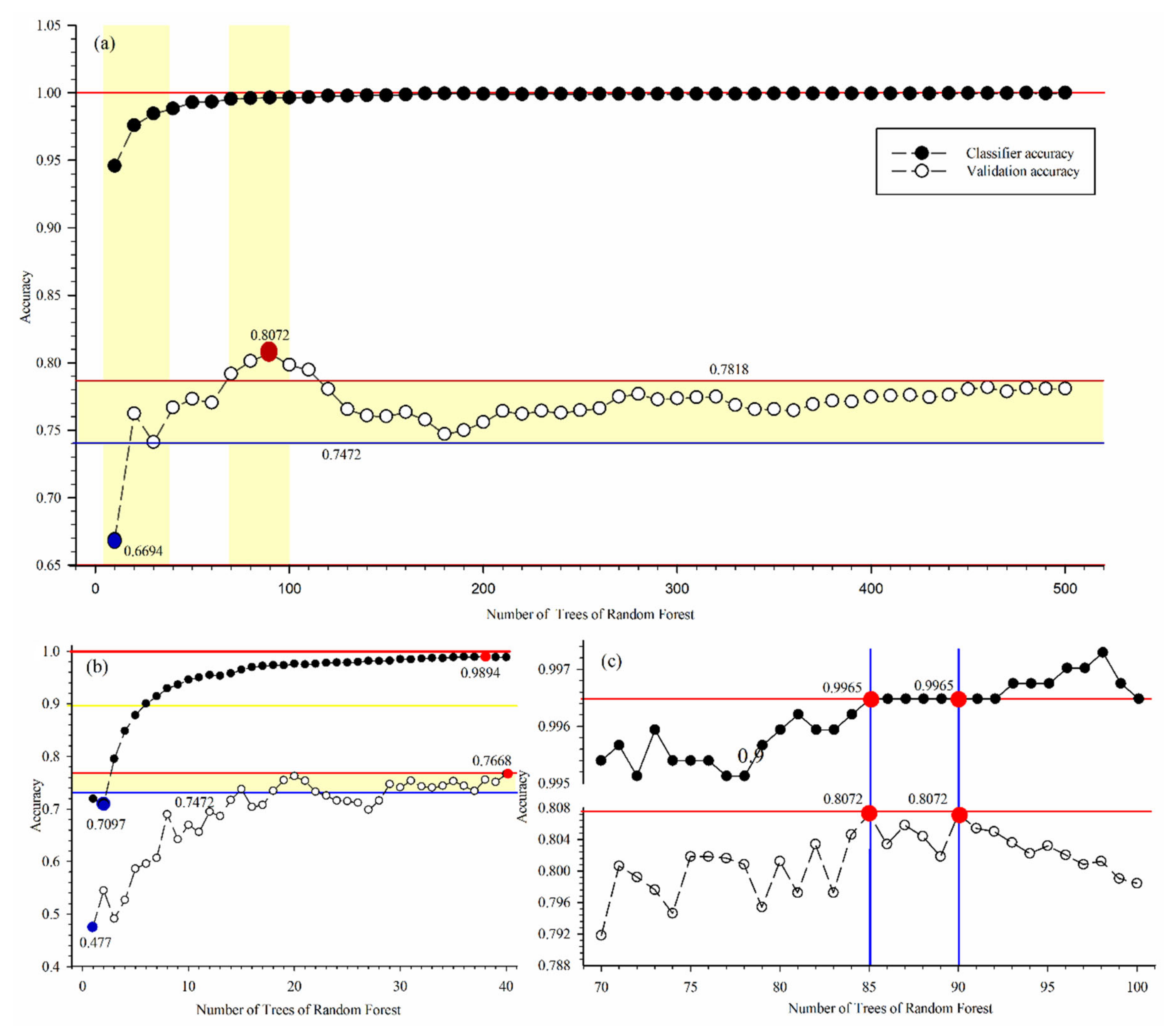
The classifier accuracy and validation accuracy for RF were different from the number of RF trees different, especially the validation accuracy. The input data were 5114 training samples dataset and 2662 testing samples dataset, and the variables were four classes (water, ice, land, and cloud). Setting variablesPerSplit, minLeafPoplation, bagFraction, outofBagMode, and seed variables of RF classifier in GEE to the default condition, many trials were conducted from 10 to 500 steps of 10 for numberofTrees variable to select the suitable and performable number of RF trees. The results are shown in Figure A1. The accuracy of the RF classifier was greater than 0.9500, except for ten trees. When the number of trees was greater than 100, the classifier accuracy was close to 1.0000. The RF classifier’s validation accuracy was between 0.7472 and 0.8072, except for ten trees, which was 0.6694.
Specifically, the validation accuracy of the RF classifier is greater than 0.7818, which ranges from 70 to 100. The largest validation accuracy was 0.8072 in 90 trees. Many trials were taken 1 step to illustrate the validation accuracy for the number of trees that ranged 10–40 and 70–100. And the results were shown in Figure A1b,c. When the number of trees was less than 40, the classifier accuracy showed a gradual upward trend, and the greatest classifier accuracy was 0.9894 in 38 trees. When the number of trees was greater than 6, the classifier accuracy was greater than a constant 0.9000. Validation accuracy showed a trend of increasing volatility. The minimum value was 0.4770 in 1 tree, and the greatest value was 0.7668 in 40 trees. When the number of trees was greater than 15, the validation accuracy values also fluctuated between 0.7472 and 0.7668. The focus was on the number of trees that ranged from 70 to 100, with the greatest validation accuracy value being 0.8072 in 85 and 90 trees, and the classifier accuracy was 0.9965. Herein, the key dependent factors were validation accuracy and high computing performance. Therefore, 85 was selected as the number of RF trees. Daily MODIS surface reflectance input into the RF classifier model, the four-class classification results of the daily image would be classed.

2.3.2. Lake Ice Threshold Value

Remote sensing extraction methods of lake ice mainly include index methods and ice threshold value methods [20,45,65,66], and many other scholars have also used visual interpretation many times [14]. Index methods were dependent on the spectral characteristics of water and ice to distinguish ice indirectly. The ice threshold value method depended on the differences between water and ice reflectances and temperature factors to distinguish ice directly. However, the most robust approaches were found to be the ice threshold value method, which used the differences in spectral bands to eliminate the atmospheric influence and system errors to some extent, and the Equation (1) is as follow:
I c e =   ρ 1 ρ 2 > a ρ 1 > b
where ρ 1 and ρ 2 represent the first band (Red) and second band (Near Infrared) of MODIS MOD09GQ. a and b are the associated threshold value parameters, where a is set to 0.028, and b is set to 0.05 [67].

2.3.3. Water Index

Many water index methods have been developed over the past several decades and used widely. This paper selects the following six commonly used water index extraction methods based on previous research literature: TCW [23], NDWI [68], MNDWI [69], AWEI [29], WI2015 [28], and MBWI [27], as shown in Table 3 [43], and compares them with RF as reference.

2.3.4. Postprocessing

The daily surface water area and ice area of Qinghai Lake were not constant but varied with time. The daily surface water area and ice area exhibited some affected values because of the clouds and haze, cloud shadow, and unfavorable illumination conditions. These factors resulted in the daily surface water coverage (surface water area divided by the total area) and ice coverage (ice area divided by the total area). Cloud filtering processing was conducted to correct some affected values, which are as follows (Figure 2).
1. If the daily surface water coverage of the lake was less than 0.01 and the daily ice coverage was greater than 0.50, this indicated no surface water and a fully iced over the lake; thus, the surface water coverage of the lake was set to 0.00, and the ice coverage was set to 1.00.
2. For the same reason, if the daily surface water coverage was greater than 0.50, the daily ice coverage was less than 0.01, indicating full surface water and no ice. Thus, the surface water coverage was set to 1.00, and the ice coverage was set to 0.00.
3. For an arbitrary three consecutive days, if the daily surface water coverage on the first day and last day were greater than 0.99, that of the midday was less than 0.99, indicating full surface water covers three consecutive days. Thus, the surface water coverage was set to 1.00, and the ice coverage was set to 0.00.
4. For an arbitrary three consecutive days, if the daily surface water coverage on the first day and last day were less than 0.01, that on midday was greater than 0.01, indicating no surface water cover occurred on the three consecutive days. Thus, the surface water coverage was set to 0.00, and the ice coverage was set to 1.00.
5. For the same reason, for an arbitrary three consecutive days, if the daily ice coverage on the first day and last day were greater than 0.99, that on midday was less than 0.99, indicating full ice cover occurred on the three consecutive days. Thus, the ice area coverage was set to 1.00, and the surface water coverage was set to 0.00.
6. For an arbitrary three consecutive days, if the daily ice coverage on the first day and last day were less than 0.01, that on midday was greater than 0.01, indicating no ice cover occurred on the three consecutive days. Thus, the ice coverage was set to 0.00, and the surface water coverage was set to 1.00.
7. The other daily surface water coverage and ice coverage that were not affected by the clouds, cloud shadow, and unfavorable illumination conditions remained unchanged.
The critical lake phenology dates for lakes undergoing freeze-thaw cycles could be better extracted based on the above daily surface water coverage and ice coverage processes. During the one ice season, the FUS date is the day before the surface water coverage begins to be less than 1.0, and the ice coverage begins to be greater than 0.0. The FUE date is when the surface water coverage decreases to 0.0, and the ice coverage increases to 1.0. The BUS date is the day before the surface water coverage begins to be greater than 0.0, and the ice coverage begins to be less than 1.0. The BUE date is when the surface water coverage increases to 1.0 and the ice coverage decreases to 0.0. The detailed critical ice phenology extraction process is shown vividly in lake phenology section. We further validated the lake phenology through the visual interpretation method due to the lack of in-situ ice observation data. According to the date-centric principle of the above critical ice phenology dates, visual interpretation was the most direct and accurate way to judge the existence of ice [4,15].

3. Results

3.1. Accuracy of RF Algorithm

The number of trees of RF was 85. Table A1 and Table A2 (Appendix B) showed training and testing accuracy. Table A1 showed the training classification results of four classes based on the confusion matrix of RF. Four class results were expressed as the pixel count, the bold count stands for the predicted accurate class results, while the accuracy of RF was expressed as the percentage. The training kappa coefficient was 99.51%, the overall training accuracy of RF was 99.65%; the agreement is almost perfect. The obtained accuracies were high for all classes. Table A2 (Appendix B) showed the testing classification results of four classes based on the confusion matrix of RF. The overall testing accuracy was 80.72%, testing the kappa coefficient was 73.45%—the agreement is almost perfect. The producer accuracies were high for four classes.

3.2. Classification of RF

The RF algorithm could classify water, ice, land, and cloud classes according to trained RF classifiers based on four classes of training samples and testing samples. Cloud cover is the greatest impact for classifying the lake water and ice. Select eight images of four seasons during the 2000/2001 and 2015/2016 ice season with cloud cover. Figure 3 visually listed the classification results and results within the water mask. There are some errors of commission When the cloud covers the land, the cloud shadow might be classified as water. Meanwhile, there are some errors of omission. When the cloud covers the lake surface water or ice, the cloud cover could be classified as the cloud and little land. Classified water and ice only occur over the lake, and some land and cloud could affect the lake surface. Daily lake water and ice inside the lake were extracted by using annual water mask products. The cloud filtering was adopted to derive the lake water coverage, lake ice coverage, and lake phenology.

3.3. Comparison of RF and Water/Ice Extraction Methods

The RF algorithm could classify both the lake’s daily surface water area and the ice area, but the ice threshold value method extracted only the lake ice area. The water index extraction methods extracted only the lake surface water area. Three cloud-free cover images were selected to visually demonstrate the advantages of the RF algorithm compared to the ice threshold value and six water index methods: a full ice cover scenario on 4 February 2001, an ice fraction and open water fraction scenario on 1 April 2001, and a full surface water cover scenario on 13 July 2001, as shown in Figure 4. Meanwhile, a comparison of water and ice areas is quantified in Table 4.
Figure 4 illustrates the full ice cover, ice fraction and open water fraction, and full surface water cover scenarios. In the first column, Figure 4a1–c1 show the raw images with bands 1, 4, and 3. Figure 4a2 shows the extracted full ice cover result of the RF algorithm, which was very consistent with Figure 4a1, where the ice area cover was 4217.50 km2, and surface water cover was 0.00 km2. Figure 4a3 shows the extracted full ice cover result from the ice threshold value method, consistent with Figure 4a1. However, the middle left was slightly omitted, the ice area cover was 4146.06 km2, and the rest of the omission area was at the middle left part. Figure 4a4–a9 showed the surface water cover results for the full ice cover scenario by water index methods consistent with the raw image’s ice cover. However, there were too many omissions based on the MBWI method: the surface water area was 2254.00 km2, and other surface water areas were 4223.25 km2, 4222.50 km2, 4295.25 km2, 4288.00 km2, and 4286.25 km2 based on the TCW, NDWI, MNDWI, AWEI, and WI2015 methods, respectively. These surface water areas were consistent with the ice area of RF.
Figure 4b2 shows the extracted ice fraction and open water fraction results obtained using the RF algorithm, consistent with Figure 4b1. The ice area cover was 2431.31 km2, the surface water cover was 1769.06 km2, the total area was 4200.37 km2, and the total area was consistent with the full ice area obtained using RF, which was 4217.50 km2. Figure 4b3 shows the extracted ice result of the ice threshold value method. The ice area was 2115.69 km2, which was consistent with the ice covers of Figure 4b1 and Figure 4b2. However, the ice cover was slightly omitted, and the surface water area was indistinct. Figure 4b4–b9 shows the surface water cover results, which were consistent with those of the raw image, but there were too many omissions by the TCW, MNDWI, and MBWI water index methods, and the surface water areas were 3742.25 km2, 4069.75 km2, and 2866.00 km2, respectively. Other surface water areas by the NDWI, AWEI, and WI2015 water index methods were 4136.50 km2, 4166.25 km2, and 4165.75 km2, respectively. These surface water areas were consistent with the ice area’s sum and surface water area by RF. However, these methods could not obtain the ice cover and surface water cover areas simultaneously.
Figure 4c2 shows the extracted full surface water cover result of the RF algorithm, which was very consistent with the raw image. The surface water cover area was 4202.69 km2, but the ice cover area showed a slight commission error of 22.00 km2. Figure 4c3 shows the extracted ice result of the ice threshold value method. The ice area was 45.25 km2, which was a commission error. Figure 4c4–c9 shows the surface water results for the full surface water cover scenario, which were consistent with the raw image, except for TCW, which showed too many omissions, and the surface water was only 1391.75 km2. The NDWI method was very consistent with the raw image, as the surface water area was 4214.00 km2; the surface water areas were 3889.50 km2, 4048.75 km2, 4051.75 km2, and 3889.50 km2 based on the MNDWI, AWEI, WI2015, and MBWI index methods, respectively, with a few omissions.

3.4. Lake Phenology

3.4.1. Lake Phenology for the 2016–2018 Ice Season

Based on the above cross-compared results, the ice threshold value method obtained only the ice area, and these water index methods obtained only the surface water area. The advantages of the RF algorithm was visually demonstrated. The RF algorithm could concurrently extract a more accurate daily surface water area and ice area. Therefore, the RF algorithm was an excellent method to accurately extract the lake’s surface water area and ice area. Furthermore, the lake’s daily surface water coverage and ice coverage and four critical ice phenology dates were calculated, as shown in Figure 2. There may be affected values in the daily surface water coverage and ice coverage; these affected values were processed using cloud filtering to obtain a more accurate dataset.
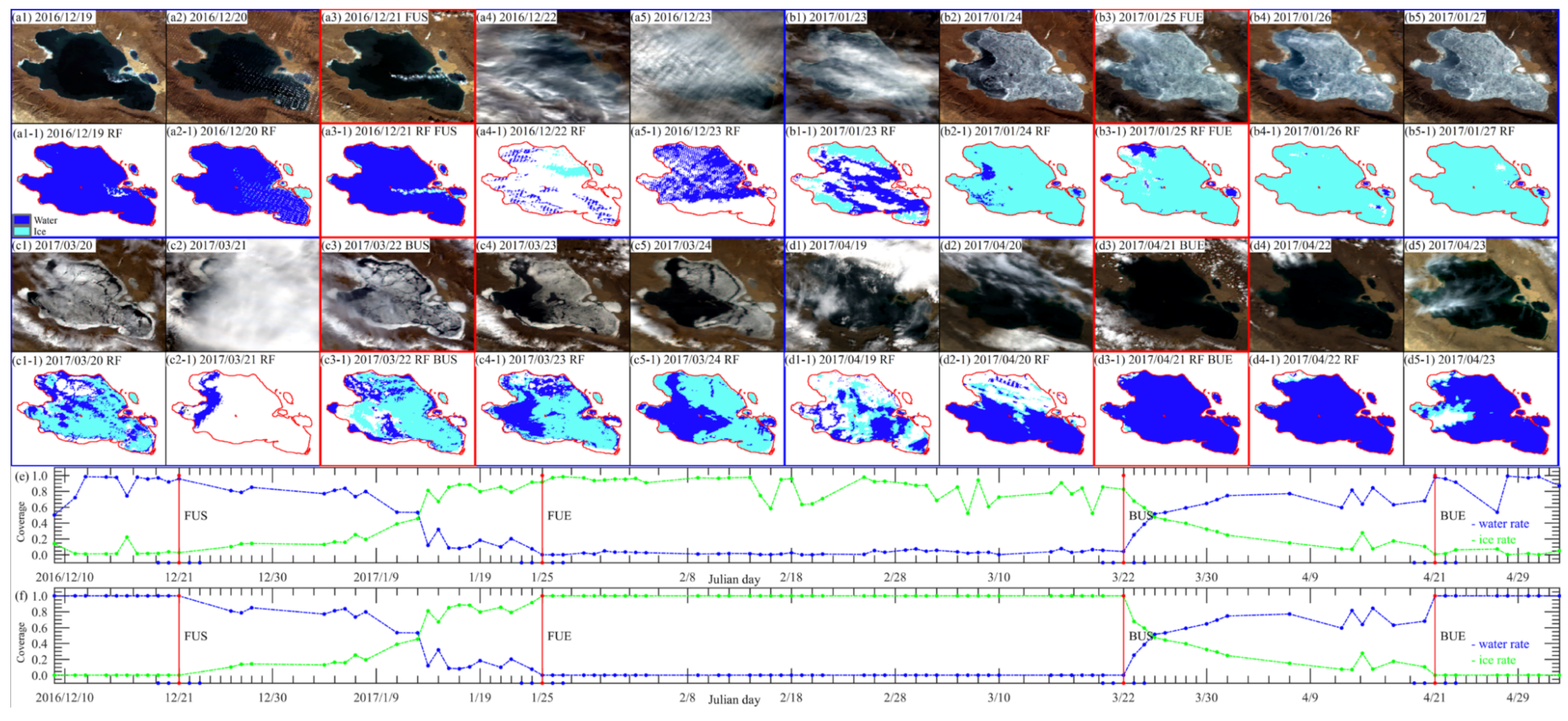
Cloud filtering processing was applied to correct the water and ice coverage and improve the accuracy of the critical ice phenology dates. To visualize the results of one full ice season using cloud filtering after using the RF algorithm, 20 raw images and the corresponding extracted water/ice cover results of RF for five adjacent dates of FUS (Figure 5a1–a5 and Figure 5a1-1 to a5-1), FUE (Figure 5b1–b5 and Figure 5b1-1 to b5-1), BUS (Figure 5c1–c5 and Figure 5c1-1 to c5-1) and BUE (Figure 5d1–d5 and Figure 5d1-1 to d5-1) during 10th Dec. 2016 to 29 April 2017 depicted the processes of four critical dates of lake phenology. Figure 5e shows the uncorrected surface water coverage and ice coverage with affected values. Figure 5f clearly shows the exact dates of FUS (Figure 5a3 and Figure 5a3-1), FUE (Figure 5b3 and Figure 5b3-1), BUS (Figure 5c3 and Figure 5c3-1) and BUE (Figure 5d3 and Figure 5d3-1) during the 2016–2017 ice season. Then, the corresponding dates were traced back to the raw images and extracted water/ice cover results to validate the critical dates, which was more reliable.
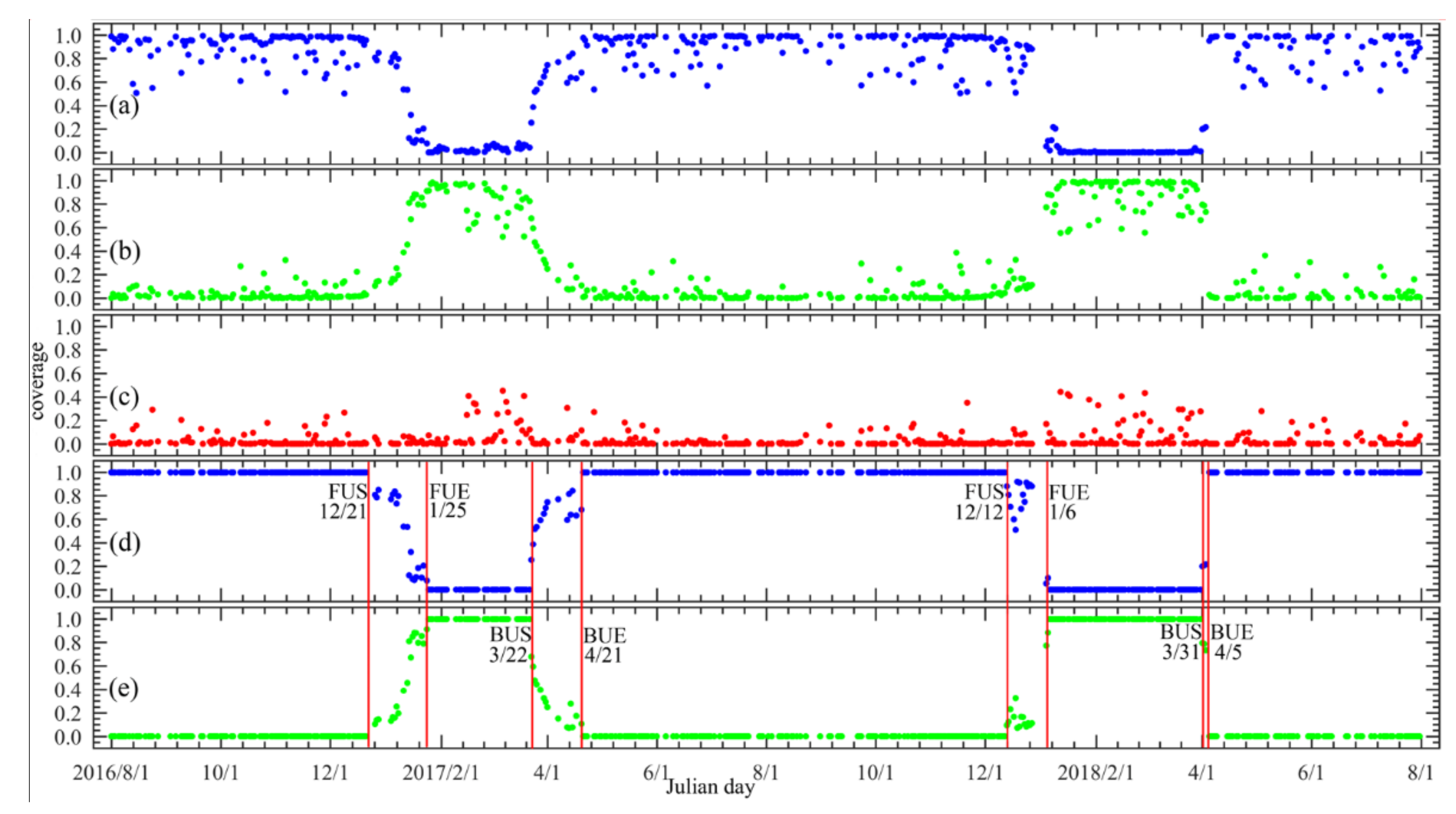
To explore the more extended periods of lake phenology, Figure 6a–c shows the daily surface water coverage, ice coverage, and cloud coverage, respectively, with affected values from 1 August 2016 to 1 August 2018. The daily surface water coverage and ice coverage was affected by cloud coverage. Some days are more severe, especially during the ice period. The extracted freeze-up and break-up event dates were not obtained. Figure 6d,e show the corrected surface water coverage and ice coverage using cloud filtering and the critical ice phenology dates during the two ice season periods.

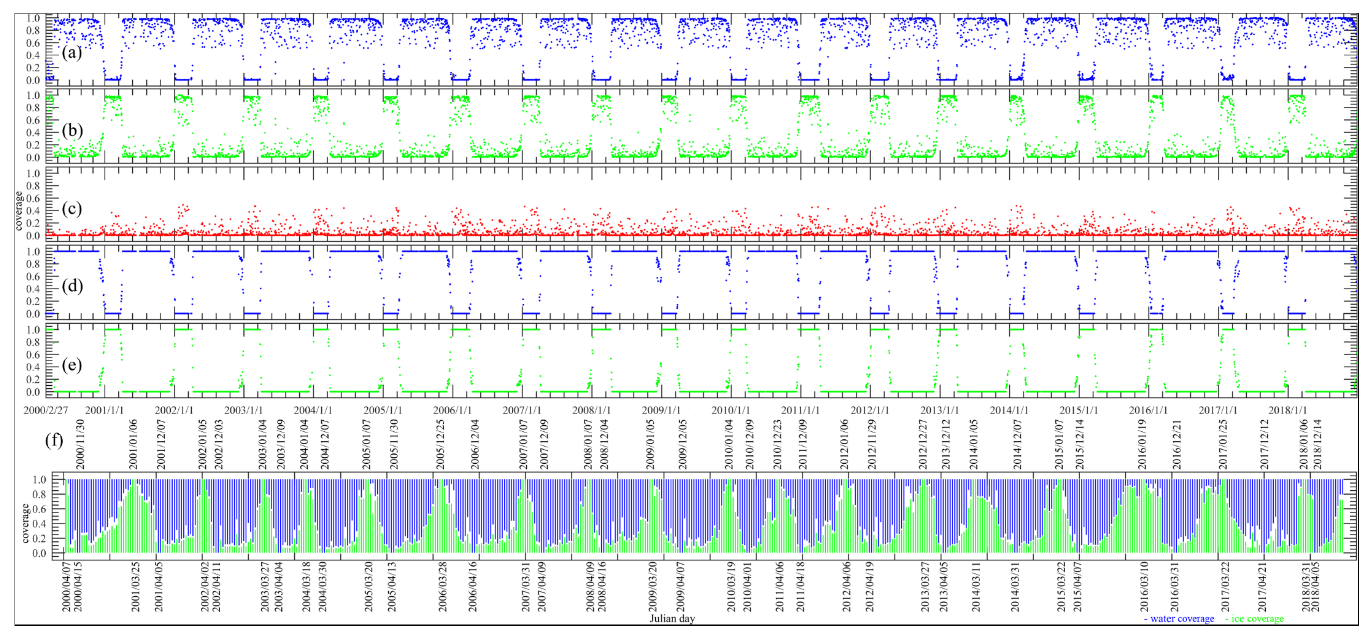
3.4.2. Lake Phenology for the 2000–2018 Ice Season

Setting the above cloud filtering as the processing criteria of uncorrected daily surface water coverage and ice coverage of all images ranged from 2000 to 2018, Figure 7a–c shows the uncorrected surface water coverage, ice coverage, and cloud coverage. The daily cloud coverage of all images was about 0.0. Only some days could be greater than 0.2, mainly the ice period. And Figure 7d,e shows the corrected surface water coverage and ice coverage using cloud filtering. Four critical dates for each ice season were extracted from the above results. Figure 7f shows the surface water coverage and ice coverage during each freeze-up and break-up event period. The four critical dates of lake phenology for each ice season are depicted on the horizontal axis, known as the Julian day, with FUS and FUE on the upper horizontal axis and BUS and BUE on the lower horizontal axis. Table A3 (Appendix B) shows the date results of critical ice phenology from 2000 to 2018.

3.5. Validation

The visual interpretation method was applied to these images with the possible representation of these dates from visible imagery to recognize the four critical dates during the 2000–2018 period. According to the date-centric principle of the critical ice phenology dates, the MODIS remote sensing images were selected. Appling visual interpretation method to validate the corresponding critical ice phenology date. When the persistent cloudiness occurs, two cloudless or less clouded MODIS images at the front and back were judged. The comparison is between the extracted dates using RF and the extracted dates using the visual interpretation method during the 2000–2018 period (Figure 8). Figure 8a shows the comparison dates of FUS, where R2 was 0.82, root mean square error (RMSE) was 2.33 days, the mean value of visual interpretation was 340.16 days; the mean value of RF was 341.89 days, and FUS was approximately early December. Approximately half of the points were on the 1:1 line, and other points were above the 1:1 line. The dates of FUS using RF were slightly greater than those using visual interpretation, with the most considerable difference in 2018 and a later Julian day in 2015–2017. Figure 8b shows the comparison dates of FUE, with an R2 of 0.93, RMSE of 2.17 days, the mean value of visual interpretation of 372.00 days, the mean value of RF of 370.78 days, and FUE was approximately early January. Only one point was above the 1:1 line, and the other points were on or below the 1:1 line; the dates of FUE using RF were slightly less than those using visual interpretation, and the Julian day was later in 2015–2016.
Figure 8c shows the comparison dates of BUS, with an R2 of 0.84, RMSE of 3.65 days, the mean value of visual interpretation of 82.11 days, the mean value of RF of 85.37 days, and the BUS was approximately late March. Approximately half of the points were on the 1:1 line. The other points were above the 1:1 line; the dates of BUS using RF were slightly greater than those using visual interpretation, with the most considerable difference in 2014 and an earlier Julian day in 2014–2016. Figure 8d shows BUE’s comparison, with an R2 of 0.90, RMSE of 2.33 days, the mean value of visual interpretation of 99.79 days, the mean value of RF of 99.32 days, and the BUE was approximately early April. Nearly all points were on the 1:1 line, and other points were below the 1:1 line, except one point above the line. The dates of BUE using RF were very close to those using visual interpretation, with the most considerable difference in 2015 and an earlier Julian day in 2014–2016. The dates of BUS and FUS using RF were slightly overestimated, with a value of 2.50 days, and the dates of the BUE and FUE using RF were somewhat underestimated, with a value of 0.85 days. Figure 8e shows the overall results were excellent, the R2 of 0.99, RMSE of 3.81 days. The dates using RF were slightly overestimated, and the value was 0.85 days. Thus, the critical ice phenology dates extracted using RF were highly credible.

4. Discussion

4.1. Trends in Lake Phenology

The availability of critical ice phenology dates for each ice season illustrated the critical events of the freeze-thaw cycle changes in Qinghai Lake (Figure A2). The four continuous freeze-thaw cycle processes are as follows: (1) surface water freeze-up, (2) full ice cover, (3) ice break-up, and (4) full surface water cover. Since the MODIS images were affected by cloud cover, the results were shown in Figure 6 and Figure 7. The cloud coverage brought the water and ice coverage errors, resulting in underestimating of the water and ice coverage. Cloud filtering procedures were applied to improve the water and ice coverage so that the sum is equal to 1. According to the above results, four critical ice phenology dates were calculated. Figure A2 shows the availability of critical events and delayed/advanced rates for the lake’s freeze-thaw cycles during 2000–2018. Statistical significance was estimated. The p-value of FUS, FUE, and BUE were 0.001, 0.001 and 0.006. Only the p-value of BUS was 0.207, as well as, the error bars to every point illustrate the associated uncertainty of the critical ice phenology. The mean dates of FUS, FUE, BUS, and BUE were Julian day 341.89, 370.78, 85.37, and 99.32, respectively. The delayed rates of FUS and FUE were 0.62 days/year and 0.48 days/year, respectively. The advanced rates of BUS and BUE were 0.48 days/year and 0.07 days/year, respectively. The FUS and FUE dates were delayed by 11.21 and 8.21 days, respectively. The BUS and BUE dates were advanced by 8.59 and 1.26 days, respectively, during 2000–2018.

4.2. LST and Lake Phenology

Temperature is a crucial driver of global climate change and extreme hydrological events. Lake surface conditions respond dramatically to climate change [70,71,72]. Changes of temperature could change the dates of freeze-up and break-up events; 0 °C isotherms have proven to be an effective temperature index connected to lake ice phenology [73,74]. The availability of LST derives from MODIS is relatively convenient due to the lack of meteorological data for a long time, and there is a strong agreement between LST and air temperature on a flat surface, such as lake surface [51,52,75]. The lake phenology dates could be predicted if some temperature variables from LST were captured. LST was derived from the lake’s surface mean temperature (day and night). The daily LST would interact on the lake surface, causing critical ice phenology changed. To delineate LST correlations and the four critical ice phenology variables (FUS, FUE, BUS, and BUE), two key indicators, DFNLST and DFPLST, were proposed after repeated and numerous calculations and comparative analysis experiments.
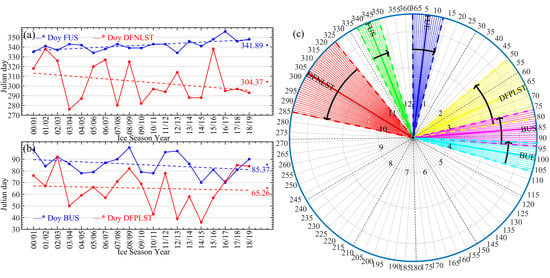
Because DFNLST is ahead of FUS, and DFPLST is ahead of BUS, focus on the correlation between these two above. Figure 9a,b illustrate the correlation and availability between the critical DFNLST and FUS and between the DFPLST and BUS for the freeze-thaw cycle emphatically during 2000–2018, respectively. Figure 9a shows that the DFNLST presented a decreasing trend and a negative relationship with FUS, with a coefficient of −0.34. The discovery of this phenomenon was an exciting find. The mean value was Julian day 304.37, which was approximately 37 days before the FUS, revealing that the first negative LST (cold air) occurs increasingly earlier. Figure 9b showed that the DFPLST also presented a decreasing trend and positive relationship with BUS, with a coefficient of 0.38. A mean value of Julian day 65.26, which was approximately 20 days before the BUS, revealing that the first positive LST (warm air) occurs increasingly earlier. Sapna Sharma [76] illustrated the widespread loss of lake ice around the Northern Hemisphere in a global warming world. Shilong Piao [77] mentioned that Spring and Autumn temperatures over the northern latitudes having risen by approximately 1.1 °C and 0.8 °C over the past two decades, where the availabilities of FUS, BUS, and DFPLST were consistent with the temperature changes. However, the DFNLST availability was not consistent, because the QTP was more sensitive than other regions to LST changes under global climate change. The first cold air outbreak cooling events occurred increasingly earlier in Autumn, and simultaneously, the first warm air outbreak event occurred increasingly earlier in Spring, and the DFNLST and DFPLST trends were the opposite of the trends of mean temperatures in Autumn and Spring in the northern hemisphere [78]. The difference may lie in the use of region scale versus hemisphere scale; another cause may be derived from the strong seasonal climate variations, which involve interactions between the warm Indian monsoon and cold westerlies [79]. Therefore, two newly proposed key indicators, DFNLST and DFPLST, enabled the determination of six critical dates versus the four critical lake phenology dates.
The changing trend and variation varied widely for the six critical dates of lake phenology. Figure 9c shows a changing trend in detail, with a range of variations and average values for the critical DFNLST, FUS, FUE, DFPLST, BUS, and BUE dates freeze-thaw cycle of Qinghai Lake during 2000–2018. The variation in DFNLST ranged from the middle of October to late November, with corresponding Julian day ranging from 284.69 to 324.05. The average Julian day was 304.37, the amplitude was 19.68 days, and the changing trend began earlier. These changing trends may result from Asian monsoons and atmospheric circulation patterns [80]. The FUS variation ranged from the beginning of December to the middle of December, with corresponding Julian day ranging from 336.55 to 347.23. The average Julian day was 341.89, the amplitude was 5.34 days, and the changing trend was delayed. The variation in FUE ranged from the end of December to the middle of January, with corresponding Julian day ranging from 363.54 to 13.02. The average was Julian day 5.78, the amplitude was 7.24 days, and the changing trend was also delayed. The variation in DFPLST ranged from late February to late March, with the corresponding Julian day ranging from 49.70 to 80.82. The average was Julian day 65.26, the amplitude was 15.56 days, and the changing trend occurred earlier. The BUS variation ranged from the middle of March to early April, with the corresponding Julian day ranging from 76.74 to 94.00. The average was Julian day 85.37, the amplitude was 8.63 days, and the changing trend occurred earlier. The BUE variation ranged from the beginning of April to the middle of April, with the corresponding Julian day ranging from 92.51 to 106.13. The average was Julian day 99.32, the amplitude was 6.81 days, and the changing trend also occurred earlier. The above change trends are consistent with studies that imply a hot future [81,82].
The LST sum between any two critical dates and the correlation between them would be further discussed. Meanwhile, 0 °C isotherms based on a 30-day average would be explored in future research work. There are still many defects in the present research and discussion, and more details would be discussed in future research works.

5. Conclusions

The focus of this research was on the lake phenology of the freeze-thaw cycle in lakes. Qinghai Lake was selected as a case study. MODIS products were used during 2000–2018, RF extracted lake surface and ice areas, the ice threshold value, and six water index (TCW, NDWI, MNDWI, AWEI, WI2015, and MBWI) methods. The optimal number of RF trees was 85. The validation accuracy value was 0.8072, the classifier accuracy was 0.9965, and comparisons found that the RF algorithm was more applicable and performed better for the freeze-thaw cycles in lakes. After applying postprocessing to address the affected values of daily lake surface water/ice/cloud coverage, the four critical ice phenology dates were correctly extracted. The results were validated using the visual interpretation method. The R2 was 0.99, the BUS and FUS dates were overestimated by 2.50 days, the BUE and FUE dates using RF were underestimated by 0.85 days, and the total was overestimated by 0.85 days. Thus, the FUS, FUE, BUS, and BUE dates extracted using RF were credible.
The mean FUS, FUE, BUS, and BUE dates were Julian day 341.89, 370.78, 85.37, and 99.32. The delayed rates of FUS and FUE were 0.62 days/year and 0.48 days/year, respectively. And the advanced rates of BUS and BUE were 0.48 days/year and 0.07 days/year, respectively. The FUS and FUE dates presented delays of 11.21 days and 8.21 days, respectively, and the BUS and BUE dates occurred 8.59 days and 1.26 days earlier, respectively, during 2000-2018. The consideration of two newly proposed key indicators, DFNLST and DFPLST, enabled the use of six critical dates that influence lake phenology. DFNLST presented a decreasing trend and a negative relationship with FUS. DFPLST also presented a decreasing trend and a positive relationship with BUS and revealed that the first negative LST (cold air)/first positive LST (warm air) occurs increasingly earlier.
The results of this study demonstrate the high performance of the RF machine learning algorithm in GEE for lake phenology, as well as the availability of four critical dates and two key proposed dates for freeze-thaw cycles in lakes. The DFNLST and DFPLST values required rigorous discussion and theoretical support. The relationships between these two indicators and other critical dates call for further research field involvement and scientific investigations. The cloudy pixels should be accounted for, and the lake surface with cloud cover could be filled and reconstructed.

Author Contributions

Conceptualization, W.H., C.H. and H.D.; methodology, W.H.; software, W.H.; validation, W.H. and H.D.; formal Analysis, W.H. and H.D.; investigation, W.H. and H.D.; resources, C.H.; data curation, W.H.; writing—original draft preparation, W.H.; writing—review & editing, C.H., H.D., J.G. and J.H.; visualization, W.H.; supervision, C.H.; project administration, C.H. and J.H.; funding acquisition, C.H., J.G. and J.H. All authors have read and agreed to the published version of the manuscript.

Funding

This work is supported by the Strategic Priority Research Program of the Chinese Academy of Sciences “CAS Earth Big Data Science Project” (Project No. XDA19040500), the Open Foundation of MOE Key Laboratory of Western China’s Environmental System, Lanzhou University “Water information extraction of Qinghai Lake based on remote sensing images” (Project No. lzujbky-2017-kl01), and the National Natural Science Foundation of China under Grants (41671375, 41871251, 41971326 and 41861047).

Acknowledgments

We are grateful for using the Google Earth Engine platform and MODIS data in this study.

Conflicts of Interest

The authors declare no conflict of interest.

Appendix A

DFNLST: Date of the first negative daily mean land surface temperature, with three consecutive days from after the ice break-up event ends to before the next surface water freeze-up event starts, which usually ranges from 1 October to the following 1 January. This term explains the length of time to the date of the start of freeze-up and illustrates how the LST controls the surface water freeze-up events.
DFPLST: date of the first positive daily mean land surface temperature, with three consecutive days from after the surface water freeze-up event ends to before the ice break-up event starts, which usually ranges from 1 February to 15 April. This term explains the length of time to the date of the start of break-up and illustrates how the LST controls the lake ice break-up events.

Appendix B

Table A1. Training confusion matrix and accuracy of RF for four classes (The bold count stands for the predicted accurate class results; The accuracy of RF was expressed as the percentage).
PredictedProducer
Accuracy/%
WaterIceLandCloud
ActualWater153770199.48
Ice29090199.67
Land101871299.84
Cloud02277999.49
Overall accuracy: 99.65
Kappa coefficient: 99.51
Table A2. Testing confusion matrix and accuracy of RF for four classes (The bold count stands for the predicted accurate class results; The accuracy of RF was expressed as the percentage).
PredictedProducer
Accuracy/%
WaterIceLandCloud
ActualWater68433533584.97
Ice31424613876.53
Land49507624983.74
Cloud30255927970.99
Overall accuracy: 80.72
Kappa coefficient: 73.45
Table A3. The detailed freeze-thaw dates of Qinghai Lake from 2000 to 2018 (the MODIS data processed between 24 February 2000 and 31 December 2018).
Ice SeasonFUSFUEBUSBUE
1999/2000 2000/04/072000/04/15
2000/20012000/11/302001/01/062001/03/252001/04/05
2001/20022001/12/072002/01/052002/04/022002/04/11
2002/20032002/12/032003/01/042003/03/272003/04/04
2003/20042003/12/092004/01/042004/03/182004/03/30
2004/20052004/12/072005/01/072005/03/202005/04/13
2005/20062005/11/302005/12/252006/03/282006/04/16
2006/20072006/12/042007/01/072007/03/312007/04/09
2007/20082007/12/092008/01/072008/04/092008/04/16
2008/20092008/12/042009/01/052009/03/202009/04/07
2009/20102009/12/052010/01/042010/03/192010/04/02
2010/20112010/12/092010/12/232011/04/062011/04/18
2011/20122011/12/092012/01/062012/04/062012/04/19
2012/20132012/11/292012/12/272013/03/272013/04/05
2013/20142013/12/122014/01/052014/03/112014/03/31
2014/20152014/12/072015/01/072015/03/222015/04/07
2015/20162015/12/142016/01/192016/03/102016/03/31
2016/20172016/12/212017/01/252017/03/222017/04/21
2017/20182017/12/122018/01/062018/03/312018/04/05
2018/20192018/12/14
Figure A1. The classifier and validation accuracy with the number of RF trees ((a). the classifier and validation accuracy with the number of RF trees during 10–500; (b). 0–40; and (c). 70–100, where the red dot represents the maximum, and the blue dot represents the minimum).
Remotesensing 12 04098 g0a1
Figure A2. The availability of critical dates of FUS, FUE, BUS and BUE, mean values, and delayed/advanced rates (red dotted lines represent the value ranging from the minimum value to the maximum value, red bar represent the error of each point).
Remotesensing 12 04098 g0a2

References

  1. Messager, M.L.; Lehner, B.; Grill, G.; Nedeva, I.; Schmitt, O. Estimating the volume and age of water stored in global lakes using a geo-statistical approach. Nat. Commun. 2016, 7, 13603. [Google Scholar] [CrossRef] [PubMed]
  2. Woolway, R.I.; Merchant, C.J. Intralake Heterogeneity of Thermal Responses to Climate Change: A Study of Large Northern Hemisphere Lakes. J. Geophys. Res. Atmos. 2018, 123, 3087–3098. [Google Scholar] [CrossRef]
  3. Hanrahan, J.L.; Kravtsov, S.V.; Roebber, P.J. Connecting past and present climate variability to the water levels of Lakes Michigan and Huron. Geophys. Res. Lett. 2010, 37. [Google Scholar] [CrossRef]
  4. Ke, C.-Q.; Tao, A.-Q.; Jin, X. Variability in the ice phenology of Nam Co Lake in central Tibet from scanning multichannel microwave radiometer and special sensor microwave/imager: 1978 to 2013. J. Appl. Remote. Sens. 2013, 7, 073477. [Google Scholar] [CrossRef]
  5. Ma, R.; Yang, G.; Duan, H.; Jiang, J.; Wang, S.; Feng, X.; Li, A.; Kong, F.; Xue, B.; Wu, J. China’s lakes at present: Number, area and spatial distribution. Sci. China Earth Sci. 2011, 54, 283–289. [Google Scholar] [CrossRef]
  6. Qiu, J. China: The third pole. Nature 2008, 454, 393–396. [Google Scholar] [CrossRef] [Green Version]
  7. Kling, G.; Hayhoe, K.; Johnson, L.; Magnuson, J.; Polassky, S.; Robinson, S.; Shuter, B.; Wander, M.; Wubbles, D.; Zak, D. Confronting Climate Change in the Great Lakes Region: Impacts on Our Communities and Ecosystems; The Union of Concerned Scientists and The Ecological Society of America: Cambridge, MA, USA, 2003; Volume 1, pp. 7–9. [Google Scholar]
  8. Zhu, L.; Xie, M.; Wu, Y. Quantitative analysis of lake area variations and the influence factors from 1971 to 2004 in the Nam Co basin of the Tibetan Plateau. Chin. Sci. Bull. 2010, 55, 1294–1303. [Google Scholar] [CrossRef]
  9. Yu, G.; Xue, B.; Wang, S.; Liu, J. Lake records and LGM climate in China. Chin. Sci. Bull. 2000, 45, 1158–1164. [Google Scholar] [CrossRef]
  10. Yong-jian, D.; Shi-yin, L.; Bai-sheng, Y.; Lin, Z. Climatic implications on variations of lakes in the cold and arid regions of China during the recent 50 years. J. Glaciol. Geocryol. 2006, 28, 623–632. [Google Scholar]
  11. Palecki, M.A.; Barry, R.G. Freeze-up and Break-up of Lakes as an Index of Temperature Changes during the Transition Seasons: A Case Study for Finland. J. Clim. Appl. Meteorol. 1986, 25, 893–902. [Google Scholar] [CrossRef]
  12. Huang, W.; Zhang, J.; Leppäranta, M.; Li, Z.; Cheng, B.; Lin, Z. Thermal structure and water-ice heat transfer in a shallow ice-covered thermokarst lake in central Qinghai-Tibet Plateau. J. Hydrol. 2019, 578, 124122. [Google Scholar] [CrossRef]
  13. Chaouch, N.; Temimi, M.; Romanov, P.; Cabrera, R.; McKillop, G.; Khanbilvardi, R. An automated algorithm for river ice monitoring over the Susquehanna River using the MODIS data. Hydrol. Process. 2014, 28, 62–73. [Google Scholar] [CrossRef]
  14. Latifovic, R.; Pouliot, D. Analysis of climate change impacts on lake ice phenology in Canada using the historical satellite data record. Remote Sens. Environ. 2007, 106, 492–507. [Google Scholar] [CrossRef]
  15. Kropáček, J.; Maussion, F.; Chen, F.; Hoerz, S.; Hochschild, V. Analysis of ice phenology of lakes on the Tibetan Plateau from MODIS data. Cryosphere 2013, 7, 287–301. [Google Scholar] [CrossRef] [Green Version]
  16. Wei, J.; Huang, W.; Li, Z.; Sun, L.; Zhu, X.; Yuan, Q.; Liu, L.; Cribb, M. Cloud detection for Landsat imagery by combining the random forest and superpixels extracted via energy-driven sampling segmentation approaches. Remote Sens. Environ. 2020, 248, 112005. [Google Scholar] [CrossRef]
  17. Zhu, Z.; Woodcock, C.E. Object-based cloud and cloud shadow detection in Landsat imagery. Remote Sens. Environ. 2012, 118, 83–94. [Google Scholar] [CrossRef]
  18. Buehler, S.A.; Kuvatov, M.; Sreerekha, T.R.; John, V.O.; Rydberg, B.; Eriksson, P.; Notholt, J. A cloud filtering method for microwave upper tropospheric humidity measurements. Atmos. Chem. Phys. 2007, 7, 5531–5542. [Google Scholar] [CrossRef] [Green Version]
  19. Duguay, C.R.; Bernier, M.; Gauthier, Y.; Kouraev, A. Remote sensing of lake and river ice. Remote Sens. Cryosphere 2015, 12, 273–306. [Google Scholar]
  20. Qiufang, W.; Qinghua, Y. Review of lake ice monitoring by remote sensing. Prog. Geogr. 2010, 29, 803–810. [Google Scholar]
  21. Dorofy, P.; Nazari, R.; Romanov, P. Application of dynamic threshold in a lake ice detection algorithm. Am. J. Rem. Sens. 2018, 6, 64–73. [Google Scholar] [CrossRef]
  22. Liu, Z.; Yao, Z.; Wang, R. Automatic identification of the lake area at Qinghai–Tibetan Plateau using remote sensing images. Quat. Int. 2019, 503, 136–145. [Google Scholar] [CrossRef]
  23. Crist, E.P. A TM Tasseled Cap equivalent transformation for reflectance factor data. Remote Sens. Environ. 1985, 17, 301–306. [Google Scholar] [CrossRef]
  24. Yang, Y.; Liu, Y.; Zhou, M.; Zhang, S.; Zhan, W.; Sun, C.; Duan, Y. Landsat 8 OLI image based terrestrial water extraction from heterogeneous backgrounds using a reflectance homogenization approach. Remote Sens. Environ. 2015, 171, 14–32. [Google Scholar] [CrossRef]
  25. Gao, B.-C. NDWI—A normalized difference water index for remote sensing of vegetation liquid water from space. Remote Sens. Environ. 1996, 58, 257–266. [Google Scholar] [CrossRef]
  26. Yue, H.; Liu, Y.; Haoren, W.; Zhang, W. Analysis of Dynamic Change of Hongjiannao Lake Based on MNDWI; IOP Publishing: Bristol, UK, 2017; Volume 57, p. 012005. [Google Scholar]
  27. Wang, X.; Xie, S.; Zhang, X.; Chen, C.; Guo, H.; Du, J.; Duan, Z. A robust Multi-Band Water Index (MBWI) for automated extraction of surface water from Landsat 8 OLI imagery. Int. J. Appl. Earth Obs. Geoinf. 2018, 68, 73–91. [Google Scholar] [CrossRef]
  28. Fisher, A.; Flood, N.; Danaher, T. Comparing Landsat water index methods for automated water classification in eastern Australia. Remote Sens. Environ. 2016, 175, 167–182. [Google Scholar] [CrossRef]
  29. Feyisa, G.L.; Meilby, H.; Fensholt, R.; Proud, S.R. Automated Water Extraction Index: A new technique for surface water mapping using Landsat imagery. Remote Sens. Environ. 2014, 140, 23–35. [Google Scholar] [CrossRef]
  30. Elith, J.; Leathwick, J.R.; Hastie, T. A working guide to boosted regression trees. J. Anim. Ecol. 2008, 77, 802–813. [Google Scholar] [CrossRef]
  31. Breiman, L. Random Forests. Mach. Learn. 2001, 45, 5–32. [Google Scholar] [CrossRef] [Green Version]
  32. Camps-Valls, G. Machine learning in remote sensing data processing. In Proceedings of the 2009 IEEE International Workshop on Machine Learning for Signal Processing, Grenoble, France, 1–4 September 2009; pp. 1–6. [Google Scholar]
  33. Pavelsky, T.M.; Smith, L.C. Spatial and temporal patterns in Arctic river ice breakup observed with MODIS and AVHRR time series. Remote Sens. Environ. 2004, 93, 328–338. [Google Scholar] [CrossRef]
  34. Wynne, R.H.; Magnuson, J.J.; Clayton, M.K.; Lillesand, T.M.; Rodman, D.C. Determinants of temporal coherence in the satellite-derived 1987–1994 ice breakup dates of lakes on the Laurentian Shield. Limnol. Oceanogr. 1996, 41, 832–838. [Google Scholar] [CrossRef]
  35. Wynne, R.H.; Lillesand, T.M. Satellite observation of lake ice as a climate indicator-initial results from statewide monitoring in Wisconsin. Photogramm. Eng. Remote Sens. 1993, 59, 1023–1031. [Google Scholar]
  36. Maslanik, J.A.; Barry, R.G. Lake ice formation and breakup as an indicator of climate change: Potential for monitoring using remote sensing techniques. In The influence of climate change and climatic variability on the hydrologic regime and water resources. In Proceedings of the Vancouver Symposium, Vancouver, BC, Canada, 9–22 August 1987; pp. 153–161. [Google Scholar]
  37. Gorelick, N.; Hancher, M.; Dixon, M.; Ilyushchenko, S.; Thau, D.; Moore, R. Google Earth Engine: Planetary-scale geospatial analysis for everyone. Remote Sens. Environ. 2017, 202, 18–27. [Google Scholar] [CrossRef]
  38. Zhang, G.; Xie, H.; Duan, S.; Tian, M.; Yi, D. Water level variation of Lake Qinghai from satellite and in situ measurements under climate change. J. Appl. Remote Sens. 2011, 5, 053532. [Google Scholar] [CrossRef]
  39. Cai, Y.; Ke, C.-Q.; Duan, Z. Monitoring ice variations in Qinghai Lake from 1979 to 2016 using passive microwave remote sensing data. Sci. Total Environ. 2017, 607–608, 120–131. [Google Scholar] [CrossRef]
  40. Yuan, Y.; Li, D.L.; An, D. Response of water level in Qinghai Lake to climate change in the Qinghai-Xizang Plateau (in Chinese). Plat. Meteorol 2012, 31, 57–64. [Google Scholar]
  41. Li, X.-Y.; Xu, H.-Y.; Sun, Y.-L.; Zhang, D.-S.; Yang, Z.-P. Lake-Level Change and Water Balance Analysis at Lake Qinghai, West China during Recent Decades. Water Resour. Manag. 2007, 21, 1505–1516. [Google Scholar] [CrossRef]
  42. Rhode, D.; Haizhou, M.; Madsen, D.B.; Brantingham, P.J.; Forman, S.L.; Olsen, J.W. Paleoenvironmental and archaeological investigations at Qinghai Lake, western China: Geomorphic and chronometric evidence of lake level history. Quat. Int. 2010, 218, 29–44. [Google Scholar] [CrossRef]
  43. Han, W.; Huang, C.; Wang, Y.; Gu, J. Study on the Area Variation of Qinghai Lake Based on Long-Term Landsat 5/8 Multi-Band Remote Sensing Imagery. Adv. Earth Sci. 2019, 34, 346–355. [Google Scholar] [CrossRef]
  44. Ding, Y.J.; Liu, F.J. Estimating on water balance elements in the drainage basin of Qinghai Lake. Arid Land Geogr. 1993, 16, 25–30. [Google Scholar]
  45. Yin, Q.J.; Yang, Y.L. Remote sensing monitoring of Lake Qinghai based on EOS/MODIS data (in Chinese). J. Lake Sci. 2005, 17, 356–360. [Google Scholar]
  46. Che, T.; Li, X.; Jin, R. Monitoring the frozen duration of Qinghai Lake using satellite passive microwave remote sensing low frequency data (in Chinese). Chin. Sci. Bull. 2009, 54, 787–791. [Google Scholar] [CrossRef]
  47. Hewer, M.J.; Gough, W.A. Lake Ontario ice coverage: Past, present and future. J. Great Lakes Res. 2019, 45, 1080–1089. [Google Scholar] [CrossRef]
  48. Maurer, J. Overview of NASA’s Terra Satellite. 2001. Available online: http://www2.hawaii.edu/~jmaurer/terra/ (accessed on 13 December 2020).
  49. Shen, H.; Li, X.; Zhang, L.; Tao, D.; Zeng, C. Compressed Sensing-Based Inpainting of Aqua Moderate Resolution Imaging Spectroradiometer Band 6 Using Adaptive Spectrum-Weighted Sparse Bayesian Dictionary Learning. IEEE Trans. Geosci. Remote Sens. 2014, 52, 894–906. [Google Scholar] [CrossRef]
  50. Roger, P.; Vermote, E.; Ray, J. MODIS Surface Reflectance User’s Guide; Collection 6: 2015. Available online: http://modis-sr.ltdri.org (accessed on 13 December 2020).
  51. Duan, S.-B.; Li, Z.-L.; Li, H.; Göttsche, F.-M.; Wu, H.; Zhao, W.; Leng, P.; Zhang, X.; Coll, C. Validation of Collection 6 MODIS land surface temperature product using in situ measurements. Remote Sens. Environ. 2019, 225, 16–29. [Google Scholar] [CrossRef] [Green Version]
  52. Sekertekin, A.; Inyurt, S.; Yaprak, S. Pre-seismic ionospheric anomalies and spatio-temporal analyses of MODIS Land surface temperature and aerosols associated with Sep, 24 2013 Pakistan Earthquake. J. Atmos. Sol. Terr. Phys. 2020, 200, 105218. [Google Scholar] [CrossRef]
  53. Carroll, M.L.; DiMiceli, C.M.; Townshend, J.R.G.; Sohlberg, R.A.; Elders, A.I.; Devadiga, S.; Sayer, A.M.; Levy, R.C. Development of an operational land water mask for MODIS Collection 6, and influence on downstream data products. Int. J. Digit. Earth. 2017, 10, 207–218. [Google Scholar] [CrossRef]
  54. Li, X.; Shen, H.; Feng, R.; Li, J.; Zhang, L. DEM generation from contours and a low-resolution DEM. ISPRS J. Photogramm. Remote Sens. 2017, 134, 135–147. [Google Scholar] [CrossRef]
  55. Jarvis, A.; Reuter, H.I.; Nelson, A.; Guevara, E. Hole-filled seamless SRTM data V4. In International Centre for Tropical Agriculture (CIAT). 2008. Available online: http://srtm.csi.cgiar.org (accessed on 13 December 2020).
  56. Segal, M.R. Machine learning benchmarks and random forest regression. UCSF Center Bioinform. Mol. Biostat. 2004, 1, 1–14. [Google Scholar]
  57. Karlson, M.; Ostwald, M.; Reese, H.; Sanou, J.; Tankoano, B.; Mattsson, E. Mapping tree canopy cover and aboveground biomass in Sudano-Sahelian woodlands using Landsat 8 and random forest. Remote Sens. 2015, 7, 10017–10041. [Google Scholar] [CrossRef] [Green Version]
  58. Sajdak, M.; Piotrowski, O. C&RT model application in classification of biomass for energy production and environmental protection. Cent. Eur. J. Chem. 2013, 11, 259–270. [Google Scholar] [CrossRef]
  59. Ripley, B.D. Pattern Recognition and Neural Networks; Cambridge University Press: Cambridge, UK, 1996. [Google Scholar] [CrossRef]
  60. Breiman, L.; Friedman, J.; Stone, C.J.; Olshen, R.A. Classification and Regression Trees; Chapman and Hall/CRC Press: London, UK, 1984. [Google Scholar]
  61. Dahinden, C. An improved Random Forests approach with application to the performance prediction challenge datasets. Hands Pattern Recognit. Microtom. 2009, 1, 1–6. [Google Scholar]
  62. Yao, A.C.-C. Decision Tree Complexity and Betti Numbers. J. Comput. Syst. Sci. 1997, 55, 36–43. [Google Scholar] [CrossRef] [Green Version]
  63. Kass, G.V. An Exploratory Technique for Investigating Large Quantities of Categorical Data. J. R. Stat. Soc. Ser. C 1980, 29, 119–127. [Google Scholar] [CrossRef]
  64. Ture, M.; Tokatli, F.; Kurt, I. Using Kaplan–Meier analysis together with decision tree methods (C&RT, CHAID, QUEST, C4.5 and ID3) in determining recurrence-free survival of breast cancer patients. Expert Syst. Appl. 2009, 36, 2017–2026. [Google Scholar] [CrossRef]
  65. Anqi, T. Research on the Variation of Namco Lake Ice by Passive Microwave Remote Sensing; Nanjing University: Nanjing, China, 2014. [Google Scholar]
  66. Sukhija, S.; Krishnan, N.C.; Singh, G. Supervised Heterogeneous Domain Adaptation via Random Forests. In Proceedings of the Twenty-Fifth International Joint Conference on Artificial Intelligence, New York, NY, USA, 9–15 July 2016; pp. 2039–2045. [Google Scholar]
  67. Qui, M.; Yao, X.; Li, X.; An, L., Gong; Gao, Y.; Liu, J. Spatial-temporal characteristics of ice phenology of Qinghai Lake from 2000 to 2016. Acta Geogr. Sin. 2018, 73, 932–944. [Google Scholar]
  68. McFeeters, S.K. The use of the Normalized Difference Water Index (NDWI) in the delineation of open water features. Int. J. Remote Sens. 1996, 17, 1425–1432. [Google Scholar] [CrossRef]
  69. Xu, H. Modification of normalised difference water index (NDWI) to enhance open water features in remotely sensed imagery. Int. J. Remote Sens. 2006, 27, 3025–3033. [Google Scholar] [CrossRef]
  70. Feng, H.; Zou, B. Satellite-based estimation of the aerosol forcing contribution to the global land surface temperature in the recent decade. Remote Sens. Environ. 2019, 232, 111299. [Google Scholar] [CrossRef]
  71. Benson, B.J.; Magnuson, J.J.; Jensen, O.P.; Card, V.M.; Hodgkins, G.; Korhonen, J.; Livingstone, D.M.; Stewart, K.M.; Weyhenmeyer, G.A.; Granin, N.G. Extreme events, trends, and variability in Northern Hemisphere lake-ice phenology (1855–2005). Clim. Chang. 2012, 112, 299–323. [Google Scholar] [CrossRef]
  72. Woolway, R.I.; Kraemer, B.M.; Lenters, J.D.; Merchant, C.J.; O’Reilly, C.M.; Sharma, S. Global lake responses to climate change. Nat. Rev. Earth Environ. 2020, 1, 388–403. [Google Scholar] [CrossRef]
  73. Bonsal, B.R.; Prowse, T.D. Trends and Variability in Spring and Autumn 0 °C-Isotherm Dates over Canada. Clim. Chang. 2003, 57, 341–358. [Google Scholar] [CrossRef]
  74. Duguay, C.R.; Prowse, T.D.; Bonsal, B.R.; Brown, R.D.; Lacroix, M.P.; Ménard, P. Recent trends in Canadian lake ice cover. Hydrol. Process. 2006, 20, 781–801. [Google Scholar] [CrossRef]
  75. Benali, A.; Carvalho, A.C.; Nunes, J.P.; Carvalhais, N.; Santos, A. Estimating air surface temperature in Portugal using MODIS LST data. Remote Sens. Environ. 2012, 124, 108–121. [Google Scholar] [CrossRef]
  76. Sharma, S.; Blagrave, K.; Magnuson, J.J.; O’Reilly, C.M.; Oliver, S.; Batt, R.D.; Magee, M.R.; Straile, D.; Weyhenmeyer, G.A.; Winslow, L.; et al. Widespread loss of lake ice around the Northern Hemisphere in a warming world. Nat. Clim. Chang. 2019, 9, 227–231. [Google Scholar] [CrossRef]
  77. Piao, S.; Ciais, P.; Friedlingstein, P.; Peylin, P.; Reichstein, M.; Luyssaert, S.; Margolis, H.; Fang, J.; Barr, A.; Chen, A.; et al. Net carbon dioxide losses of northern ecosystems in response to autumn warming. Nature 2008, 451, 49–52. [Google Scholar] [CrossRef]
  78. Piao, S.; Friedlingstein, P.; Ciais, P.; Viovy, N.; Demarty, J. Growing season extension and its impact on terrestrial carbon cycle in the Northern Hemisphere over the past 2 decades. Glob. Biogeochem. Cycles 2007, 21. [Google Scholar] [CrossRef]
  79. Yang, K.; Yao, F.; Wang, J.; Luo, J.; Shen, Z.; Wang, C.; Song, C. Recent dynamics of alpine lakes on the endorheic Changtang Plateau from multi-mission satellite data. J. Hydrol. 2017, 552, 633–645. [Google Scholar] [CrossRef]
  80. Dai, A. Drought under global warming: A review. Wiley Interdiscip. Rev. Clim. Chang. 2011, 2, 45–65. [Google Scholar] [CrossRef] [Green Version]
  81. Andreae, M.O.; Jones, C.D.; Cox, P.M. Strong present-day aerosol cooling implies a hot future. Nature 2005, 435, 1187–1190. [Google Scholar] [CrossRef] [PubMed]
  82. Huang, Y.; Dickinson, R.E.; Chameides, W.L. Impact of aerosol indirect effect on surface temperature over East Asia. Proc. Natl. Acad. Sci. USA 2006, 103, 4371. [Google Scholar] [CrossRef] [PubMed] [Green Version]
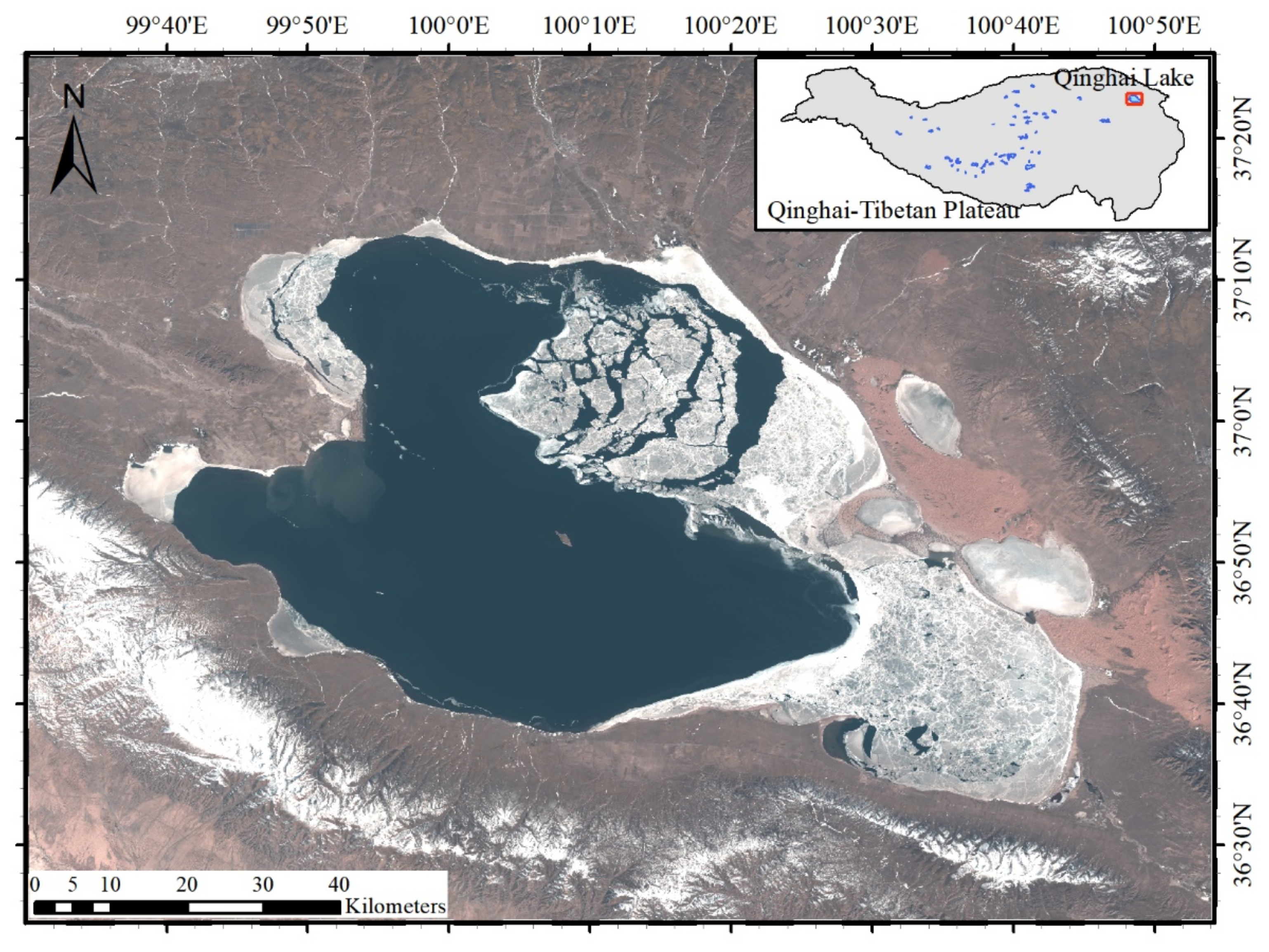
Figure 1. Location of Qinghai Lake (Landsat 8 image in 26 March 2017) and the lakes identified from the World Wildlife Fund’s Global Lake and Wetland Database (GLWD) level 1 products the Qinghai-Tibetan Plateau.
Remotesensing 12 04098 g001
Figure 2. Processing flowchart of MODIS data based on the GEE platform (ice is derived from Ice Threshold Value, and water is derived from six common water index methods. The results are compared with ice and water derived from RF. The daily ice coverage and water coverage derived from RF were processed through cloud filtering. wri: i-th day water coverage; iri: i-th day ice coverage).
Remotesensing 12 04098 g002
Figure 3. Output classes of four seasons during the 2000/2001 and 2015/2016 ice season with cloud cover for 16 October 2000 (a1,a1-1,a1-2), 9 February 2001 (a2,a2-1,a2-2), 1 April 2001 (a3,a3-1,a3-2), 17 July 2001 (a4,a4-1,a4-2), 13 October 2015 (b1,b1-1,b1-2), 20 January 2016 (b2,b2-1,b2-2), 11 April 2016 (b3,b3-1,b3-2), 16 July 2016 (b4,b4-1,b4-2).
Remotesensing 12 04098 g003
Figure 4. MODIS images with full ice cover, ice-water cover, and full water scenes and the corresponding ice/water extracted results based on several methods for 4 February 2001 (a1a9), 1 April 2001 (b2b9) and 13 July 2001 (c2c9).
Remotesensing 12 04098 g004
Figure 5. Water/ice results of RF using the cloud filtering algorithm for one full ice season from 10 December 2016 to 29 April 2017 ((a1a5). MODIS images for five consecutive days in FUS; (a1-1a5-1). Corresponding water/ice results of RF for five consecutive days in FUS; (b1b5). MODIS images for five consecutive days in FUE; (b1-1b5-1). Corresponding water/ice results of RF for five consecutive days in FUE; (c1c5). MODIS images for five consecutive days in BUS; (c1-1c5-1). Corresponding water/ice results of RF for five consecutive days in BUS; (d1d5). MODIS images for five consecutive days in BUE; (d1-1d5-1). Corresponding water/ice results of RF for five consecutive days in BUE; (e). Water coverage, ice coverage results; (f). Water coverage, ice coverage through cloud filtering. Red boxes and lines represent FUS, FUE, BUS, and BUE, and cloudy images were deleted for the following dates; 2016/12/22, 2016/12/23, 2017/01/23, 2017/03/21, and 2017/04/19).
Remotesensing 12 04098 g005
Figure 6. Water coverage, ice coverage, and cloud coverage for the two full ice season periods from 1 August 2016 to 31 July 2018 ((a). water coverage; (b). ice coverage; (c). cloud coverage; (d). water coverage through cloud filtering; (e). ice coverage through cloud filtering. Blue dot, green dot, and red dot represent water, ice, and cloud, respectively).
Remotesensing 12 04098 g006
Figure 7. Water coverage, ice coverage, and cloud coverage from 2000 to 2018 (a). water coverage; (b). ice coverage; (c). cloud coverage; (d). water coverage through cloud filtering; (e). ice coverage through cloud filtering; (f). water coverage, ice coverage, and four dates during each ice season, the bottom of the x-axis are pairs of serial BUS and BUE, and the top of the x-axis are pairs of continuous FUS and FUE for each ice season; only the freeze-up and break-up processes were displayed, full ice cover and full water cover processes were not displayed. Blue dot, green dot, and red dot represent water, ice, and cloud, respectively).
Remotesensing 12 04098 g007
Figure 8. The Julian day comparison between RF and visual interpretation (color and circle size represents the year. (a). BUS; (b). BUE; (c). FUS; (d). FUE; (e). Total results).
Remotesensing 12 04098 g008
Figure 9. The correlations and trends of DFNLST, FUS, FUE, DFPLST, BUS, and BUE dates for the freeze-thaw cycle of Qinghai Lake during 2000–2018 ((a). The correlations between DFNLST and FUS, coefficient: −0.34; (b). The correlations between DFPLST and BUS, coefficient: 0.38; (c). The range of variations of six critical dates, 1–12 represents for months inside of the circle; 5–365 represents for days outside of the circle).
Remotesensing 12 04098 g009
Table 1. The information of the MODIS former seven bands [50] (* MOD09GQ version 6: Terra Surface Reflectance Daily Global 250 m, ** MOD09GA version 6: Terra Surface Reflectance Daily L2G Global 1 km and 500 m).
Band.SpectralWavelength (nm)Resolution (m)Primary Use
* 1Red620–670250Land/Cloud/Aerosols Boundaries
* 2Near Infrared841–876250
** 3Blue459–479500Land/Cloud/Aerosols Properties
** 4Green545–565500
** 5Short Wave Infrared 11230–1250500
** 6Short Wave Infrared 21628–1652500
** 7Short Wave Infrared 32105–2155500
Table 2. Selected dates of training and testing samples in MODIS.
YearWinterSpringSummerAutumn
2000 4/157/1510/15
20011/154/167/1510/15
20021/134/167/1810/15
20031/154/157/1310/15
20041/134/157/1510/17
20051/154/157/1610/15
20061/154/167/1510/15
20071/154/157/1510/15
20081/144/157/1510/15
20091/144/157/1510/15
20101/154/167/1810/15
20111/154/157/1510/15
20121/164/147/1510/15
20131/154/157/1510/15
20141/154/157/1510/16
20151/154/157/1610/16
20161/154/167/1610/16
20171/154/157/1510/14
20181/14,12/234/157/151015
Table 3. Six commonly used water index methods.
Water IndexEquationNo
TCW T C W = 0.0315 ρ 3 + 0.2021 ρ 4 + 0.3102 ρ 1 + 0.1594 ρ 2 0.6806 ρ 6 0.6109 ρ 7 (2)
NDWI N D W I = ρ 4 ρ 2 ρ 4 + ρ 2 (3)
MNDWI M N D W I = ρ 4 ρ 6 ρ 4 + ρ 6 (4)
AWEI A W E I = 4 ρ 4 ρ 6 0.25 ρ 2 + 2.75 ρ 7 ρ 3 + 2.5 ρ 4 1.5 ρ 2 + ρ 6 0.25 ρ 7 (5)
WI2015 W I 2015 = 1.7204 + 171 ρ 4 + 3 ρ 1 70 ρ 2 45 ρ 6 71 ρ 7 (6)
MBWI M B W I = 2 ρ 1 ρ 2 ρ 6 ρ 5 ρ 7 (7)
where ρ 1 and ρ 2 represent the first band (Red) and second band (Near Infrared) of MODIS MOD09GQ. ρ 3 ~ ρ 7 represent the third band (Blue) through the seventh band (Short Wave Infrared 3) of MODIS MOD09GA.
Table 4. Comparison of water and ice area derived from different methods on three dates.
Methods200102042001040120010713
Water Area/km2Ice Area/km2Water Area/km2Ice Area/km2Water Area/km2Ice Area/km2
RF0421717692431420222
Ice Threshold-4146-2115-45
TCW4223-3742-1391-
NDWI4222-4136-4214-
MNDWI4295-4069-3889-
AWEI4288-4166-4048-
WI20154286-4165-4051-
MBWI2254-2866-3889-
Publisher’s Note: MDPI stays neutral with regard to jurisdictional claims in published maps and institutional affiliations.