Technical Note

An LSWI-Based Method for Mapping Irrigated Areas in China Using Moderate-Resolution Satellite Data

1
Guangdong Ecological Meteorology Center, Guangzhou 510640, China
2
Center for Monsoon and Environment Research, Guangdong Province Key Laboratory for Climate Change and Natural Disaster Studies, School of Atmospheric Sciences, Sun Yat-sen University, Zhuhai 519082, China
3
Guangzhou Institute of Tropical and Marine Meteorology/Guangdong Provincial Key Laboratory of Regional Numerical Weather Prediction, CMA, Guangzhou 510641, China
*
Author to whom correspondence should be addressed.
Remote Sens. 2020, 12(24), 4181; https://doi.org/10.3390/rs12244181
Submission received: 15 November 2020 / Revised: 10 December 2020 / Accepted: 17 December 2020 / Published: 21 December 2020
(This article belongs to the Special Issue Satellite Hydrological Data Products and Their Applications)

Abstract

:
Accurate spatial information about irrigation is crucial to a variety of applications, such as water resources management, water exchange between the land surface and atmosphere, climate change, hydrological cycle, food security, and agricultural planning. Our study proposes a new method for extracting cropland irrigation information using statistical data, mean annual precipitation and Moderate Resolution Imaging Spectroradiometer (MODIS) land cover type data and surface reflectance data. The approach is based on comparing the land surface water index (LSWI) of cropland pixels to that of adjacent forest pixels with similar normalized difference vegetation index (NDVI). In our study, we validated the approach over mainland China with 612 reference samples (231 irrigated and 381 non-irrigated) and found the accuracy of 62.09%. Validation with statistical data also showed that our method explained 86.67 and 58.87% of the spatial variation in irrigated area at the provincial and prefecture levels, respectively. We further compared our new map to existing datasets of FAO/UF, IWMI, Zhu and statistical data, and found a good agreement with the irrigated area distribution from Zhu’s dataset. Results show that our method is an effective method apply to mapping irrigated regions and monitoring their yearly changes. Because the method does not depend on training samples, it can be easily repeated to other regions.

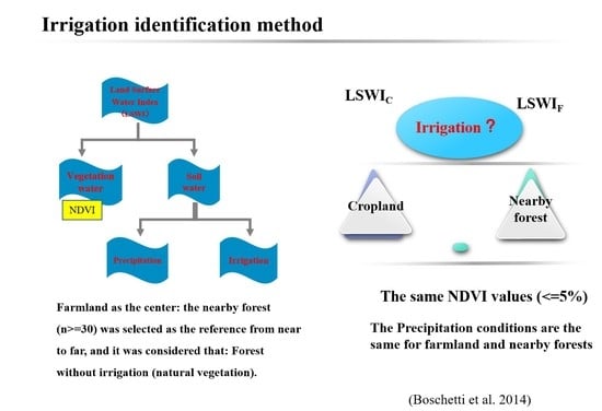
Graphical Abstract

1. Introduction

Irrigation plays a vital role in increasing global grain output [1], especially in regions lacking fresh water. In the past 40 years, global crop production has doubled, cropland has increased by 12%, and irrigation has expanded [2]. Although only 18% of the world’s arable land is irrigated [3], 40% of the global grain output comes from irrigated agriculture [4]. Irrigated agriculture accounts for the primary consumption in fresh water resources, using more than 70% of groundwater, rivers and lakes [5]. Irrigation information is very important for a wide range of studies, including water exchange between the atmosphere and the land surface [6,7], agriculture water requirements and supply [8], allocation of water resources between agriculture and ecosystems [9,10,11], hydrological processes [12], environmental concerns such as soil quality depletion [13,14], agriculture-climate interactions and feedback [15,16]. Therefore, accurate information on irrigation distribution is an important step in monitoring cropland yields and water resources [17]. Accurate mapping of China’s irrigated areas will not only help the Chinese government better assess future food and water security issues, but also help guide future policies aimed at mitigation or adaptation to climate change. Therefore, we need a deep understanding of agricultural policies and land management practices to identify irrigation information [18]. Although irrigation is important for energy, water cycles and food security [19,20], the precise distribution and location of irrigated croplands in the world remains uncertain [21]. Therefore, more objective and convenient methods are needed to be developed on irrigation information extraction [18,22,23,24,25].
Remote sensing is a widely used tool for monitoring irrigated croplands [7,17,26,27,28]. Satellite sensors have been used for monitoring irrigation at local, regional, continental, and global scales [22,23,24,26,27,28,29,30,31,32,33,34,35,36]. Monitoring irrigation through satellite remote sensing data has become common, but mapping irrigation at large scales remains relatively rare. So far, there are only four products providing information about the distribution of irrigated areas at the global scale. The Global Map of Irrigation Areas version 5.0 (GMIA 5.0), produced by the Food and Agriculture Organization and the University of Frankfurt (FAO/UF), has a spatial resolution of 5′ and reflects the irrigation percentage from 2000 to 2008 [25,37,38,39,40]. The MIRCA2000 product is based on the GMIA products, with the objective to cover all major food crops irrigated areas [18], but does not represent the actual irrigation area. The Global Irrigated Area Map (GIAM) accounts for sub-pixel irrigation intensity at 1 km spatial resolution [40], which is produced by the International Water Management Institute (IWMI) [24,40,41,42], but it may provide less reliable due to limited ground-truth data in the training samples. The Global Rain-fed, Irrigated, and Paddy Croplands (GRIPC) map (500 m), was the highest spatial resolution among the other three maps [35]. All these four products are more suitable to be applied at the global rather than the local scale [43,44,45,46,47], because of the limited ground data available to verify them, and temporal changes in irrigated areas change [34]. Census data on irrigation may also be uncertain because of political reasons, particularly in developing countries [48].
There are two common approaches for identifying irrigation with remote sensing data: digital image classification and visual interpretation. Early work focused on temporal spectral signature trends differences between irrigated farmland and other land use or land cover [49,50]. A strong spectral separation of the electromagnetic spectrum has been found from irrigated and harvested fields and fallow land in the near-infrared and visible portions, which makes the automatic method widely used in the visual interpretation of satellite data [51,52]. Compared with visual interpretation, the digital image classification relies on spectral conversion [53,54]. Due to faster analysis and lower costs associated with mapping, digital image classification is usually applied in numerous irrigation mapping studies. Common classification methods include density slicing with thresholds [54], decision tree classifications [55,56], multi-stage classification [57,58,59], and unsupervised classification clustering [30].
Currently, remote sensing is the most effective method for identifying irrigation information, saving time and money, with high accuracy compared to traditional statistical methods [17]. It provides temporal frequencies and spectral data to monitor vegetation growth, maturity, and yield [60,61,62]. Compared with traditional statistical surveys method, remote sensing data are more convenient due to their digital nature, lower cost, and faster processing. Remote sensing monitoring of irrigation is particularly valuable in developing countries with limited funds and relatively little objective information. In addition, compared with statistical data provided for administrative units, remote sensing data provides more accurate information on the location and extend of irrigated cropland. This is of great importance for prioritizing water supplies, assessing the environmental impacts of irrigation, and providing information on irrigation intensity and location change.
A new method was developed for identifying irrigated areas using 500-m MODIS data in our study. The goal of our study were: (1) to develop a new method to identify irrigated areas; (2) to verify the performance of our new method using observation sites and statistical data at the provincial and prefecture levels; (3) to calculate the area and map the spatial distribution of irrigated areas in China. Our new method can provide accurate irrigation location and contribute to improved agricultural research.

2. Materials and Methods

2.1. Study Area

Our study area is mainland China, with a land area of about 9.6 million square kilometers (Figure 1). Mountains, hills, and plateaus account for about 70% of China. In addition, only 15% of the land area can be cultivated by humans. Most arable land is concentrated in the east of China, especially the North China Plain, the Northeast China, the Guanzhong Plain, the middle and lower reaches of Yangtze River, the Pearl River Delta, and big basins. Nearly 45% of China’s cropland is irrigated [63]. Available water resources and arable land are distributed unevenly in China. Agricultural irrigation consumes the greatest amount of the fresh water resources every year. The planting methods vary from south to north, including single cropping, double cropping, three crops in two years, and three crops a year. China is divided into wet regions, semi-humid regions, semi-arid regions and arid regions. Mean annual precipitation increases from the northwest to the southeast coast, which varies from 531.3 to 2939.7 mm [64].

2.2. Preprocessing of the MODIS Data and Precipitation Data

The MODIS images were downloaded from website of the Land Processes Distributed Active Archive Center (LPDAAC). Land surface water index (LSWI) (bands 2 and 6) and Normalized Difference Vegetation Index (NDVI) (bands 1 and 2) were calculated using MODIS eight-day surface reflectance products (MOD09A1). The Savitzky–Golay filter was used to smooth the noise in the vegetation index time series, especially the noise related to atmospheric variability and cloud contamination [65]. Land cover types were determined based on the Global vegetation classification system of the International Geosphere-Biosphere Programme included in the MCD12Q1 products. The gridded daily precipitation dataset was from Yuan et al. (2015) [66]. This dataset was on the basis of the meteorological observations data of 735 meteorological stations in the National Climate Center of the China Meteorological Administration (CMA), and the gridded climate dataset (10 × 10 km) is interpolated by using the method of thin plate smoothing splines [66]. We resampled the precipitation dataset to match with the MODIS data.

2.3. Site-Based Irrigation Data

Figure 1 shows the spatial distribution of the validation samples in mainland China. For our study we collected 612 validation samples that were from three sources. First, the soil moisture and crop growth dataset was provided by the China Meteorological Data Sharing Service System (CMDSSS). Sites were used from this source, were a total of 214 non-irrigated and 158 irrigated samples. Second, they were field surveys, which were carried out from July to August of 2016 in mainland China—76 non-irrigated samples and 46 irrigated samples. Third, it was collected by Google Earth, with the irrigation information on large, irrigated regions. We collected 612 evaluation samples (231 irrigated samples and 381 non-irrigated samples). At all sampling sites, we carried out a survey and recorded on cropland irrigation times, fertilizer use and pesticide, well depth, and crop yield.

2.4. Validation and Comparison

In our study, regression analysis is done using computer software (SPSS Statistics 17.0.1). A central part of the regression output of such packages is a summary of the foregoing information in an Analysis of Variance, or ANOVA table. We matched the ground records listed in Section 2.3 with remote sensing data and analyze them. In addition, we contrasted the estimated irrigation areas from our method with statistical data at prefecture and province scales. The data were collected from the National Bureau of Statistics of China [64]. We contrasted our new irrigation map with three widely used irrigation datasets: Zhu datasets, FAO/UF, and IWMI. We resampled our new irrigation map and IWMI datasets to the same spatial resolution with FAO/UF datasets.

2.5. Methodology

The principle of our method was to determine irrigated areas by comparing the canopy vegetation moisture index of a cropland site with the nearby natural vegetation (i.e., forests). Our method was based upon two fundamental assumptions: (1) temporal soil moisture of irrigated croplands is higher than in non-irrigated croplands or natural vegetation (i.e., forests) [23,67]. In general, at the non-irrigated croplands sites or natural vegetation, precipitation is the only soil moisture source, and soil moisture will keep decreasing between precipitation events, which may lead to relatively low levels of soil moisture. (2) Differences in moisture between croplands and adjacent forests decrease as the precipitation increases. The less precipitation a site receives, the larger the difference between cropland and adjacent forests in moisture, which is caused by increased artificial irrigation for the need of higher yield.
To validate the first assumption, LSWI was used as an indicator of soil moisture conditions in our study, and we calculated the mean value of LSWI (LSWIC) during the growing season at each cropland pixel to show the condition of land surface moisture. The calculation formula of LSWI is:
L S W I = ρ n i r ρ s w i r ρ n i r + ρ s w i r
where ρswir and ρnir represent short wave infrared and red reflectances, respectively [68]. We calculated LSWIC from the 201st to the 241st day at all 612 investigated cropland samples, including 231 irrigated and 381 non-irrigated samples, and contrasted LSWIC with those of nearby forests (LSWIF). Moreover, because there is a significant positive correlation relationship between LSWI and NDVI [22,69], we compared the LSWI of cropland and forest with the same NDVI values to rule out the influence of NDVI [68]. The land cover type data was from MCD12Q1. At a given cropland pixel, we selected the nearest 30 forest pixels to contrast, which the mean NDVI (NDVIF) value is equal to NDVI of croplands (NDVIC) (i.e., |NDVIC-NDVIF|< 0.05 × NDVIC). Then, we computed the mean LSWI value (201st to 241st day) of nearby forests (LSWIF), and contrasted LSWIC with all investigated cropland sites to test the first assumption.
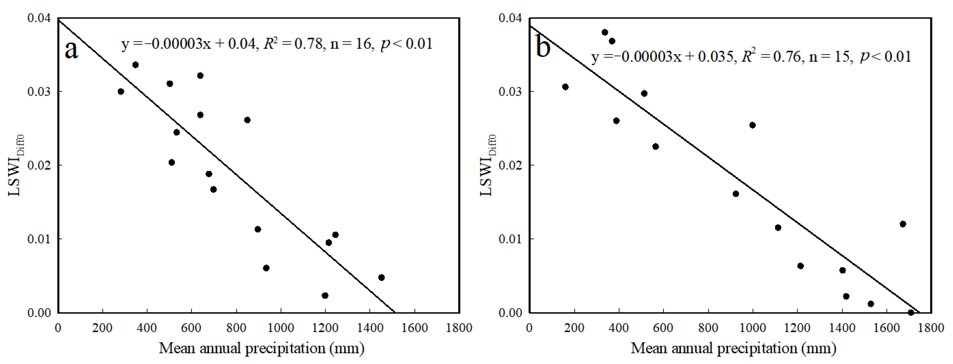
To test our second assumption, in every province, we selected and ranked all pixels by descending the LSWI differences between LSWIF and LSWIC (LSWIDiff =LSWIC − LSWIF). The pixels near the front in the sort had bigger LSWIDiff values, and hence a larger probability of being recognized as irrigated cropland pixel. We used statistical data at province-level to determine the LSWIDiff thresholds through calculate the number (N) of pixels with the biggest LSWIDiff as irrigated pixels. The LSWIDiff value of the Nth is called the threshold (LSWIDiff0) for distinguishing the irrigated pixels and non-irrigated pixels. We used 16 provinces (half the number of Chinese provinces) to test the relationship between mean annual precipitation and LSWIDiff0 raised by our second assumption. In addition, we used the remaining 15 provinces (other half the number of Chinese provinces) to validate this relationship. The results for testing our two assumptions were showed in Figure 2 and Figure 3. If our assumptions were verified that there is a significant correlation relationship between mean annual precipitation and LSWIDiff0, we can deduce LSWIDiff0 for every province based on this correlation equation. After the LSWIDiff0 was calculated, we can judge the cropland pixels which LSWIDiff value is bigger than LSWIDiff0 as irrigated pixels.
Based on our two assumption, we established the following six steps to select irrigated cropland pixels:
Step (1) We calculated the mean LSWI (LSWIC) and NDVI (NDVIC) values of each cropland pixel from day 201 to day 241 of the year, which correspond to the peak of growing season of the year.
Step (2) Using the land cover product (MCD12Q1), we identified cropland (class 12) and forest pixels (classes 1, 2, 3, 4, 5); based on nearby forest pixels with average NDVI value (NDVIF) close to NDVIC (i.e., |NDVIF − NDVIC| < 0.05 × NDVIC) during the same investigated periods, we calculated the LSWI difference (LSWIDiff = LSWIC − LSWIF) for every cropland pixel.
Step (3) Within a given province, we sorted all pixels with LSWIDiff by descending order. The pixels with larger LSWIDiff values were more likely to be irrigated. Statistical data of irrigation areas at province-level from the National Bureau of Statistics were used to calculate the LSWIDiff thresholds. The N pixels with the largest LSWIDiff were selected as irrigated; we determined whether the total area of the N pixels equated to the recorded statistical area of irrigation for a given city.
Step (4) We selected half of the provinces identified in Step 3 to determine the LSWI thresholds. We investigated the correlations between the LSWIDiff thresholds and mean annual precipitation, and found a significant negative linear relationship between LSWIDiff thresholds and mean annual precipitation.
Step (5) Using the appropriate LSWIDiff0 thresholds in other half provinces to verify our regression equation. Then, we used mean annual precipitation as input parameter for the regression equation to deduce the threshold value (LSWIDiff0) for every pixel. If LSWIDiff is greater than the deduced threshold (LSWIDiff0), then the pixel is considered to be irrigated.
Step (6) These five steps were repeated until the total pixels of mainland China were compared and identified. The pixels of all irrigated areas were combined to obtain the irrigated map of the study area.
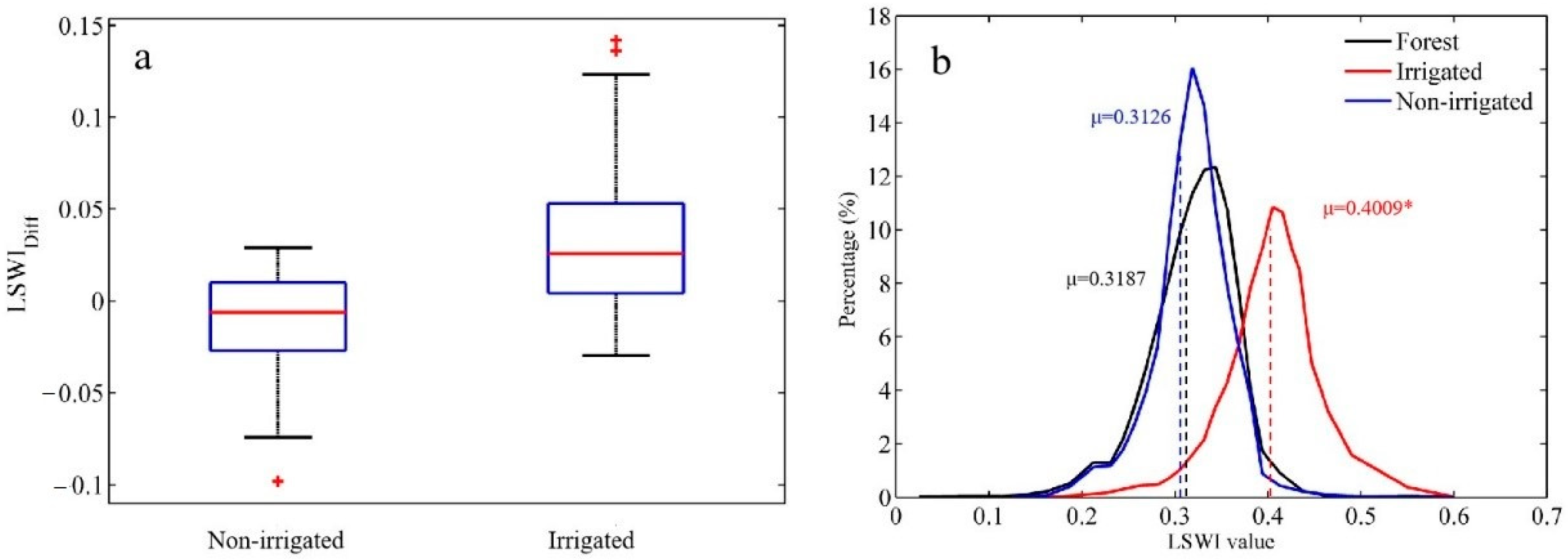
We checked the first assumption that LSWI values of the irrigated cropland pixels were bigger than those of the nearby natural forest vegetation pixels. Therefore, we compared LSWI values of the investigated sampling sites with the nearby forests pixels that have the equivalent NDVI values with the cropland pixels. There was an obvious LSWI difference between the irrigated and non-irrigated cropland pixels compared to the nearby natural forest vegetation pixels (ANOVA test, p < 0.01) (Figure 2a).
We examined the second assumption proposed in the methodology section based on statistics data of irrigation and the mean annual precipitation. A significant negative linear relationship was found between the mean annual precipitation and LSWIDiff0 thresholds (the LSWI difference between the nearby forest and irrigated cropland) (p < 0.01) (Figure 3). The LSWIDiff0 thresholds decreased with the increasing mean annual precipitation, indicating that the larger LSWI differences occurred in dry regions, which confirmed our second assumption. Hence, we used the regression to calculate the thresholds (LSWIDiff0) for all provinces using mean annual precipitation.

3. Results

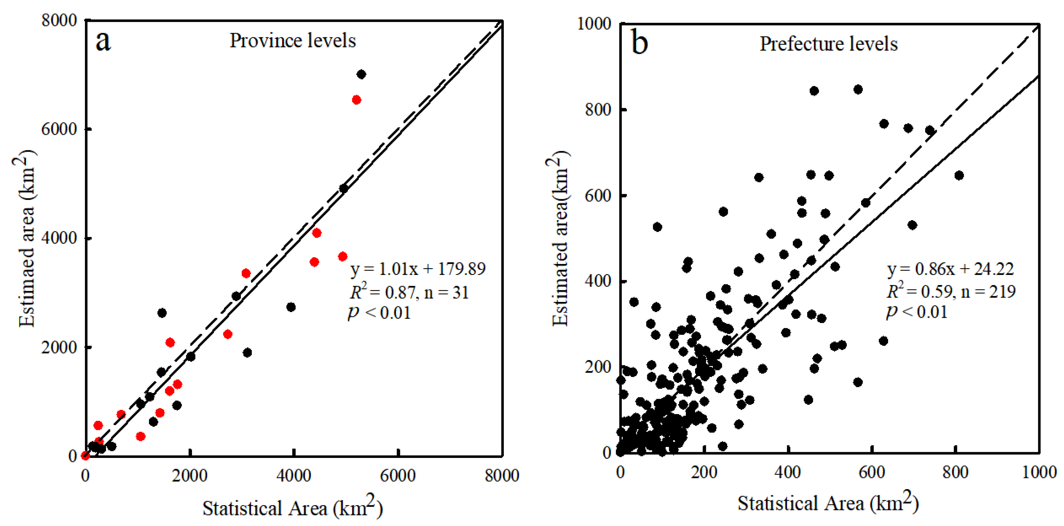
We used the statistical data to validate our method at the prefecture and the province levels. The results show that our new method can accurately identify irrigated areas compared to the statistical data at the two spatial scales (i.e., the prefecture and the provincial levels) (Figure 4). The coefficients of determination (R2) between the estimated irrigated areas in our method and the statistical data areas were 0.59 (Figure 4b) and 0.87 (Figure 4a) at the prefecture and province levels, respectively. Estimated irrigated areas were highly consistent with the statistical data over the 16 provinces used to build the regression relation between LSWIDiff0 and the mean annual precipitation, as shown in Figure 3a. Furthermore, the agreement between estimated areas and statistical data was also found over the remaining 16 provinces (Figure 4a), indicating a good relationship between irrigated areas estimated by our method and the statistical data.
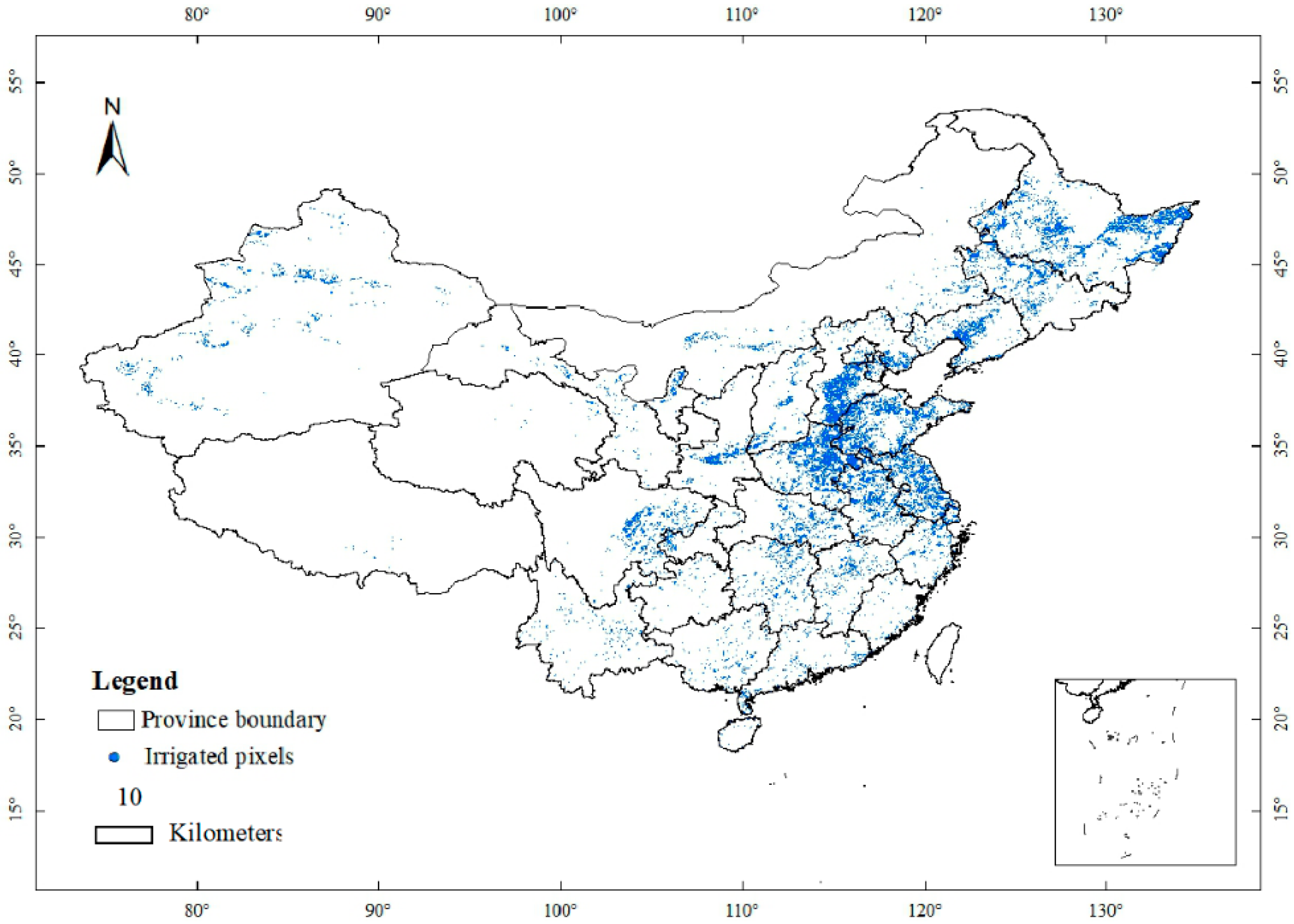
Based on the remote sensing canopy moisture index, we produced a map of spatial distribution of irrigated regions in mainland China (Figure 5). Irrigated regions are distributed mainly in three alluvial plains (the middle and lower reaches of the Yangtze River Plain, the North China Plain, and the Northeast Plain) and valleys along five rivers (Yangtze River Basin, Liaohe River Basin, Yellow River Basin, Haihe River Basin, Huaihe River Basin, Songhua River Basin). The irrigated area of these three alluvial plains accounts for most of the irrigated area of China. The National Bureau of Statistics of China [64] reported 654,387 km2 of irrigated area in China 2016, while we estimated 604,344 km2 (Table 1) [64]. The overall irrigated area in China was underestimated by 7.64%.
To evaluate the accuracy of our method, we made comparisons with three other irrigation datasets: the irrigation map derived by Zhu et al. (2015) [70] (see method) and two global irrigation datasets (IWMI and FAO/UF). In total, the overall accuracies are 41.18, 58.98, 61.76, and 62.09% in FAO/UF, IWMI, Zhu’s dataset and our map (Table 2).
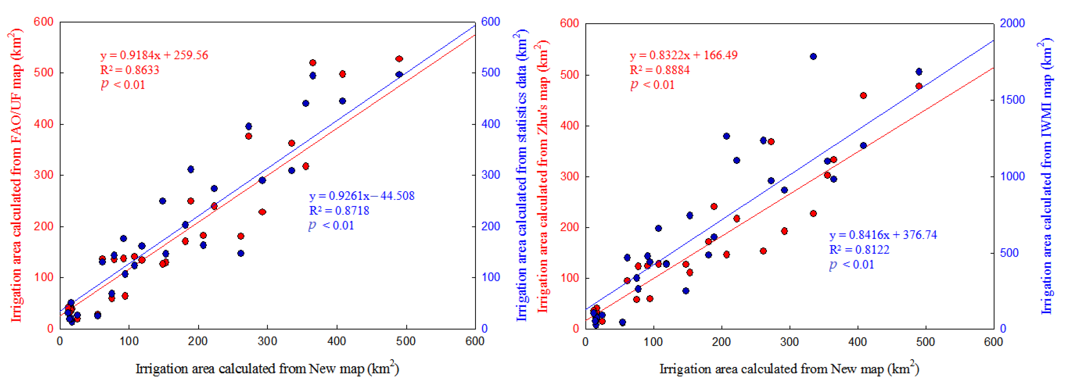
To compare the datasets, we calculated the irrigated areas at the provincial level from four irrigation maps. Figure 6 indicates the scatter plots for inter-comparison of four maps and statistical data. The two scatter plots show that the map obtained from our study is more similar to Zhu’s map than FAO/UF map and IWMI map and is more consistent with the statistical data of irrigated area at provincial level.
To further compare similarity/dissimilarity among the four maps, we aggregated them at the prefecture-level (Figure 7). This figure shows that both FAO/UF map and our map show irrigation patterns with similar types of spatial distribution. The Hetao plain, the Northeast plain, the North China plain, and Northwestern plain of Xinjiang province have the largest irrigated fields in China. Southeastern and southwestern China have the smallest irrigated fields in China. The largest discrepancy between irrigation distribution derived by our map and the FAO/UF map is in Heilongjiang, Xinjiang, Jiangsu, Henan, and Liaoning Province.

4. Discussion

Mapping irrigation distribution is challenging because the water source for croplands may be represented by precipitation, irrigation, or both. Based on phenological characteristics, this research developed a new method to identify irrigation by analyzing MODIS, precipitation and statistical data. In our study, natural vegetation forest was used as a reference to compare the LSWI of cropland and the nearby forests with equal NDVI. Our method is especially suitable for China, where nearly 70% of the land area are mountains, plateaus, and hills. We discovered the regression coefficient relationship between the LSWIDiff0 thresholds (the difference in LSWI between nearby forests and irrigated cropland) and mean annual precipitation. Our method is based on this relationship to identify irrigated regions and the regression coefficients we used in mainland China are shown in Figure 3. These regression coefficients may change with different climatic backgrounds. Therefore, if the method is extended to other regions, the relationship between LSWIDiff0 and mean annual precipitation needs to be redefined.
However, there are also two weaknesses in our method. First, the method does not take into account the differences in water storage between forests and croplands. In general, the nearby forests turn green earlier than the fields [71,72]. Thus, there may be differences in soil moisture between cropland and forest, since forests that were reforested earlier can store more precipitation in the soil [73,74]. In addition, previous studies have shown that plants in different ecosystems have different transpiration capacities and water retention capacities under the same leaf area index (LAI) [75,76]. The differences of transpiration between croplands and forest plants may lead to the differences in soil moisture.
Second, it is clear that our approach is most likely to perform better in arid regions than in humid regions, where rainfall is plentiful and the supplemental irrigation may be the main form of irrigation [70]. Supplemental irrigation usually takes place in a short period of crop growth and development, and temporal spectral differences of the additional soil moisture brought by irrigation are not obvious. However, as irrigation contributes to higher crop yields, irrigation requirements are closely related to climatic conditions. Our method used precipitation data and time series of NDVI and LSWI to estimate the presence of irrigation in each cropland pixel. We emphasized the level of mean annual precipitation, which aims at reflecting irrigation needs, and average LSWI conditions, to reflect the moisture index differences between irrigated cropland and nearby non-irrigated forests. In humid regions, our method may perform worse than the traditional classification methods, but it still provides an alternative irrigation assessment method.
Our method presents some advantages. Our method does not rely on field investigation and is easily scaled and applied to a larger region. In our method, irrigated pixels can be automatically identified just through the MODIS land-cover product, avoiding visual interpretation [70,77,78] of high-resolution images [79] and much field work [80,81]. This advantage may substantially improve the repeatability and applicability of our method. Standardization of the procedure allows it to be easily repeated in other similar areas all over the world and used to map real-time irrigation areas as long as the latest remote sensing data can be obtained.

5. Conclusions

In our study, we developed a new method for identifying irrigated areas in mainland China, based on the regression between the mean annual precipitation and the LSWI difference between cropland and the adjacent forest pixels, which were identified from the MODIS land cover datasets. We calculated the regression relation between the threshold of irrigation and mean annual precipitation at provincial levels. Validation of the irrigation map derived by our method and statistical data at provincial and prefecture levels indicated that the approach was reliable. We further collected 612 reference samples (231 irrigated and 381 non-irrigated samples) to validate our new irrigation map for mainland China at the pixel level. The overall accuracy of our new map is 62.09%. Based on statistical data, validation indicated that our method explained 86.67 and 58.87% of the spatial variation in irrigated areas at the provincial and prefecture levels, respectively. Results suggest that our method is an effective and promising tool for mapping irrigated regions. Moreover, the accurate mapping of irrigated regions, especially in arid and semi-arid regions, will be beneficial for studying the effects of human activities on agroecosystems and their relationships with global changes.

Author Contributions

K.X. was the main author of the manuscript. L.W. provided some valuable suggestions. W.Y. and Y.D. supervised and provided logistical support to the research and modified the manuscript. All authors have read and agreed to the published version of the manuscript.

Funding

This study was Funded by National Natural Science Foundation of China (41801326) and National Key Basic Research Program of China (2016YFA0602701), Youth Program of National Natural Science Foundation of China (41705140).The APC was funded by National Natural Science Foundation of China.

Acknowledgments

We also thank Minna Ma, Zhuoxuan Liang and Qu Ling for their help of data processing.

Conflicts of Interest

The authors declare no conflict of interest.

References

  1. Grogan, D.S.; Zhang, F.; Prusevich, A.; Lammers, R.B.; Wisser, D.; Glidden, S.; Li, C.; Frolking, S. Quantifying the link between crop production and mined groundwater irrigation in China. Sci. Total Environ. 2015, 511, 161–175. [Google Scholar] [CrossRef] [Green Version]
  2. Gleick, P.H. Global Freshwater Resources: Soft-Path Solutions for the 21st Century. Science 2003, 302, 1524–1528. [Google Scholar] [CrossRef] [Green Version]
  3. Food and Agriculture Organization of the United Nations (FAO): FAO Statistical Databases (FAOSTAT). 2005. Available online: http://faostat.fao.org/ (accessed on 18 December 2020).
  4. United Nations Commission on Sustainable Development (UNCSD). Comprehensive Assessment of the Freshwater Resources of the World; Report E/CN.17/1997/9; UNCSD: New York, NY, USA, 1997. [Google Scholar]
  5. Wisser, D.; Frolking, S.; Douglas, E.M.; Fekete, B.M.; Vörösmarty, C.J.; Schumann, A.H. Global irrigation water demand: Variability and uncertainties arising from agricultural and climate data sets. Geophys. Res. Lett. 2008, 35, 24408. [Google Scholar] [CrossRef] [Green Version]
  6. Özdoğan, M.; Rodell, M.; Beaudoing, H.; Toll, D.L. Simulating the Effects of Irrigation over the United States in a Land Surface Model Based on Satellite-Derived Agricultural Data. J. Hydrometeorol. 2010, 11, 171–184. [Google Scholar] [CrossRef]
  7. Cammalleri, C.; Anderson, M.C.; Gao, F.; Hain, C.R.; Kustas, W.P. Mapping daily evapotranspiration at field scales over rainfed and irrigated agricultural areas using remote sensing data fusion. Agric. For. Meteorol. 2014, 186, 1–11. [Google Scholar] [CrossRef] [Green Version]
  8. Droogers, P.; Aerts, J. Adaptation strategies to climate change and climate variability: A comparative study between seven contrasting river basins. Phys. Chem. Earth Parts A/B/C 2005, 30, 339–346. [Google Scholar] [CrossRef] [Green Version]
  9. Dai, Z.; Li, Y. A multistage irrigation water allocation model for agricultural land-use planning under uncertainty. Agric. Water Manag. 2013, 129, 69–79. [Google Scholar] [CrossRef]
  10. Ge, Y.; Li, X.; Huang, C.; Nan, Z. A Decision Support System for irrigation water allocation along the middle reaches of the Heihe River Basin, Northwest China. Environ. Model. Softw. 2013, 47, 182–192. [Google Scholar] [CrossRef]
  11. Wu, X.; Zhou, J.; Wang, H.; Li, Y.; Zhong, B. Evaluation of irrigation water use efficiency using remote sensing in the middle reach of the Heihe river, in the semi-arid Northwestern China. Hydrol. Process. 2015, 29, 2243–2257. [Google Scholar] [CrossRef]
  12. Shibuo, Y.; Jarsjö, J.; Destouni, G. Hydrological responses to climate change and irrigation in the Aral Sea drainage basin. Geophys. Res. Lett. 2007, 34, 91–99. [Google Scholar] [CrossRef]
  13. Asadi, S.S.; Azeem, S.; Prasad AV, S.; Anji Reddy, M. Analysis and mapping of soil quality in Khandaleru catchment area using remote sensing and GIS. Current Sci. 2008, 95, 391–396. [Google Scholar]
  14. Metternicht, G.; Zinck, J. Remote sensing of soil salinity: Potentials and constraints. Remote Sens. Environ. 2003, 85, 1–20. [Google Scholar] [CrossRef]
  15. Sacks, W.J.; Cook, B.I.; Buenning, N.; Levis, S.; Helkowski, J.H. Effects of global irrigation on the near-surface climate. Clim. Dyn. 2009, 33, 159–175. [Google Scholar] [CrossRef] [Green Version]
  16. Shi, W.; Tao, F.; Liu, J. Regional temperature change over the Huang-Huai-Hai Plain of China: The roles of irrigation versus urbanization. Int. J. Clim. 2013, 34, 1181–1195. [Google Scholar] [CrossRef]
  17. Özdoğan, M.; Yang, Y.; Allez, G.; Cervantes, C. Remote Sensing of Irrigated Agriculture: Opportunities and Challenges. Remote Sens. 2010, 2, 2274–2304. [Google Scholar] [CrossRef] [Green Version]
  18. Portmann, F.T.; Siebert, S.; Döll, P. MIRCA2000-Global monthly irrigated and rainfed crop areas around the year 2000: A new high-resolution data set for agricultural and hydrological modeling. Glob. Biogeochem. Cycles 2010, 24, 1–24. [Google Scholar] [CrossRef]
  19. Burney, J.; Woltering, L.; Burke, M.; Naylor, R.; Pasternak, D. Solar-powered drip irrigation enhances food security in the Sudano–Sahel. Proc. Natl. Acad. Sci. USA 2010, 107, 1848–1853. [Google Scholar] [CrossRef] [Green Version]
  20. Özdoğan, M. Exploring the potential contribution of irrigation to global agricultural primary productivity. Glob. Biogeochem. Cycles 2011, 25, 1–12. [Google Scholar] [CrossRef]
  21. Vörösmarty, C.J. Global water assessment and potential contributions from Earth Systems Science. Aquat. Sci. 2002, 64, 328–351. [Google Scholar] [CrossRef]
  22. Xiao, X.; Boles, S.; Liu, J.; Zhuang, D.; Frolking, S.; Li, C.; Salas, W.A.; Moore, B. Mapping paddy rice agriculture in southern China using multi-temporal MODIS images. Remote Sens. Environ. 2005, 95, 480–492. [Google Scholar] [CrossRef]
  23. Özdoğan, M.; Gutman, G. A new methodology to map irrigated areas using multi-temporal MODIS and ancillary data: An application example in the continental US. Remote Sens. Environ. 2008, 112, 3520–3537. [Google Scholar] [CrossRef] [Green Version]
  24. Thenkabail, P.S.; Biradar, C.M.; Noojipady, P.; Dheeravath, V.; Li, Y.J.; Velpuri, M.; Gumma, M.; Gangalakunta, O.R.P.; Turral, H.; Cai, X.; et al. Global irrigated area map (GIAM), derived from remote sensing, for the end of the last millennium. Int. J. Remote Sens. 2009, 30, 3679–3733. [Google Scholar] [CrossRef]
  25. Siebert, S.; Kummu, M.; Porkka, M. A global dataset of the extent of irrigated land from 1900 to 2005. Hydrol. Earth Syst. Sci. 2015, 19, 1521–1545. [Google Scholar] [CrossRef] [Green Version]
  26. Thenkabail, P.S.; Dheeravath, V.; Biradar, C.M.; Reddy, G.O.; Noojipady, P.; Gurappa, C.; Velpuri, N.M.; Gumma, M.K.; Li, Y. Irrigated Area Maps and Statistics of India Using Remote Sensing and National Statistics. Remote Sens. 2009, 1, 50–67. [Google Scholar] [CrossRef] [Green Version]
  27. McAllister, A.; Whitfield, D.; Abuzar, M. Mapping Irrigated Farmlands Using Vegetation and Thermal Thresholds Derived from Landsat and ASTER Data in an Irrigation District of Australia. Photogramm. Eng. Remote Sens. 2015, 81, 229–238. [Google Scholar] [CrossRef]
  28. Chen, Y.; Lu, D.; Luo, L.; Pokhrel, Y.; Deb, K.; Huang, J.; Ran, Y. Detecting irrigation extent, frequency, and timing in a heterogeneous arid agricultural region using MODIS time series, Landsat imagery, and ancillary data. Remote Sens. Environ. 2018, 204, 197–211. [Google Scholar] [CrossRef]
  29. Özdoğan, M.; Woodcock, C.E.; Salvucci, G.D.; Demir, H. Changes in Summer Irrigated Crop Area and Water Use in Southeastern Turkey from 1993 to 2002: Implications for Current and Future Water Resources. Water Resour. Manag. 2006, 20, 467–488. [Google Scholar] [CrossRef] [Green Version]
  30. Biggs, T.W.; Thenkabail, P.S.; Gumma, M.K.; Scott, C.A.; Parthasaradhi, G.R.; Turral, H.N. Irrigated area mapping in heterogeneous landscapes with MODIS time series, ground truth and census data, Krishna Basin, India. Int. J. Remote Sens. 2007, 27, 4245–4266. [Google Scholar] [CrossRef]
  31. Arino, O.; Gross, D.; Ranera, F.; Leroy, M.; Bicheron, P.; Brockman, C.; Defourny, P.; Vancutsem, C.; Achard, F.; Durieux, L.; et al. GlobCover: ESA service for global land cover from MERIS. In Proceedings of the IEEE the International Geoscience and Remote Sensing Symposium, Barcelona, Spain, 23–28 July 2007; pp. 2412–2415. [Google Scholar]
  32. Thenkabail, P.S.; Parthasaradhi, G.; Biggs, T.W.; Gumma, M.K.; Turral, H. Spectral matching techniques to determine historical land use/land cover (LULC) and irrigated areas using time-series AVHRR Pathfinder datasets in the Krishna river basin, India. Photogramm. Eng. Remote Sens. 2007, 73, 1029–1040. [Google Scholar]
  33. Dheeravath, V.; Thenkabail, P.S.; Chandrakantha, G.; Noojipady, P.; Reddy, G.P.O.; Biradar, C.M.; Gumma, M.K.; Velpuri, M. Irrigated areas of India derived using MODIS 500 m time series for the years 2001–2003. ISPRS J. Photogramm. Remote Sens. 2010, 65, 42–59. [Google Scholar] [CrossRef]
  34. Brown, J.F.; Pervez, S. Merging remote sensing data and national agricultural statistics to model change in irrigated agriculture. Agric. Syst. 2014, 127, 28–40. [Google Scholar] [CrossRef] [Green Version]
  35. Salmon, J.; Friedl, M.A.; Frolking, S.; Wisser, D.; Douglas, E.M. Global rain-fed, irrigated, and paddy croplands: A new high resolution map derived from remote sensing, crop inventories and climate data. Int. J. Appl. Earth Obs. Geoinf. 2015, 38, 321–334. [Google Scholar] [CrossRef]
  36. Xiang, K.; Ma, M.; Liu, W.; Zhu, X.F.; Yuan, W.P. Mapping Irrigated Areas in Northeast China by Comparing to Natural Vegetation. Remote Sens. 2019, 11, 825. [Google Scholar] [CrossRef] [Green Version]
  37. Siebert, S.; Döll, P.; Hoogeveen, J.; Faures, J.-M.; Frenken, K.; Feick, S. Development and validation of the global map of irrigation areas. Hydrol. Earth Syst. Sci. 2005, 9, 535–547. [Google Scholar] [CrossRef]
  38. Siebert, S.; Döll, P.; Feick, S.; Hoogeveen, J.; Frenken, K. Global Map of Irrigation Areas Version 4.0.1; University of Frankfurt (Main)/Food: Frankfurt, Germany; Agriculture Organization of the United Nations: Rome, Italy, 2007. [Google Scholar]
  39. Siebert, S.; Henrich, V.; Frenken, K.; Burke, J. Global Map of Irrigation Areas Version 5.0; Rheinische Friedrich-Wilhelms-University: Bonn, Germany; Food and Agriculture Organization of the United Nations: Rome, Italy, 2013. [Google Scholar]
  40. Thenkabail, P.S.; Biradar, C.M.; Noojipady, P.; Cai, X.; Dheeravath, V.; Li, Y.; Velpuri, N.M.; Gumma, M.K.; Pandey, S.; Thenkabailc, P.S.; et al. Sub-pixel Area Calculation Methods for Estimating Irrigated Areas. Sensors 2007, 7, 2519–2538. [Google Scholar] [CrossRef] [Green Version]
  41. Thenkabail, P.S.; Biradar, C.M.; Noojipady, P.; Dheeravath, V.; Li, Y.J.; Velpuri, M. A Global Irrigated Area Map (GIAM) Using Remote Sensing at the End of the Last Millennium; International Water Management Institute: Colombo, Sri Lanka, 2008. [Google Scholar]
  42. Thenkabail, P.S.; Biradar, C.M.; Turral, H. An irrigated area map of the world (1999) derived from remote sensing. Iwmi Books Rep. 2006, 36, 600–605. [Google Scholar]
  43. Hanasaki, N.; Inuzuka, T.; Kanae, S.; Oki, T. An estimation of global virtual water flow and sources of water withdrawal for major crops and livestock products using a global hydrological model. J. Hydrol. 2010, 384, 232–244. [Google Scholar] [CrossRef]
  44. Pokhrel, Y.; Hanasaki, N.; Koirala, S.; Cho, J.; Yeh, P.J.-F.; Kim, H.; Kanae, S.; Oki, T. Incorporating Anthropogenic Water Regulation Modules into a Land Surface Model. J. Hydrometeorol. 2012, 13, 255–269. [Google Scholar] [CrossRef] [Green Version]
  45. Döll, P.; Hoffmann-Dobrev, H.; Portmann, F.; Siebert, S.; Eicker, A.; Rodell, M.; Strassberg, G.; Scanlon, B.R. Impact of water withdrawals from groundwater and surface water on continental water storage variations. J. Geodyn. 2012, 59–60, 143–156. [Google Scholar] [CrossRef]
  46. Wada, Y.; Wisser, D.; Bierkens, M. Global modeling of withdrawal, allocation and consumptive use of surface water and groundwater resources. Earth Syst. Dyn. Discuss. 2013, 4, 355–392. [Google Scholar] [CrossRef] [Green Version]
  47. Rost, S.; Gerten, D.; Bondeau, A.; Lucht, W.; Rohwer, J.; Schaphoff, S. Agricultural green and blue water consumption and its influence on the global water system. Water Resour. Res. 2008, 44, 137–148. [Google Scholar] [CrossRef] [Green Version]
  48. Giordano, M. Global Groundwater? Issues and Solutions. Annu. Rev. Environ. Resour. 2009, 34, 153–178. [Google Scholar] [CrossRef]
  49. Thelin, G.P.; Heimes, F.J. Mapping Irrigated Cropland from Landsat Data for Determination of Water Use from the High Plains Aquifer in Parts of Colorado, Kansas, Nebraska, New Mexico, Oklahoma, South Dakota, Texas, and Wyoming; U.S. Geological Survey Professional Paper; US Government Printing Office: Washington, DC, USA, 1987.
  50. Rundquist, D.; Hoffman, R.; Carlson, M.; Cook, A. The Nebraska center-pivot inventory-An example of operational satellite remote sensing on a long term basis. Photogramm. Eng. Remote Sens. 1989, 55, 587–590. [Google Scholar]
  51. Keene, K.M.; Conley, C.D. Measurement of irrigated acreage in Western Kansas from Landsat images. Environ. Geol. 1980, 3, 107–116. [Google Scholar] [CrossRef]
  52. Haack, B.; Wolf, J.; English, R. Remote sensing change detection of irrigated agriculture in Afghanistan. Geocarto Int. 1998, 13, 65–75. [Google Scholar] [CrossRef]
  53. Lenney, M.P.; Woodcock, C.E.; Collins, J.B.; Hamdi, H. The status of agricultural lands in Egypt: The use of multitemporal NDVI features derived from landsat TM. Remote Sens. Environ. 1996, 56, 8–20. [Google Scholar] [CrossRef]
  54. Starbuck, M.J.; Tamayo, J. Monitoring vegetation change in Abu Dhabi Emirate from 1996 to 2000 and 2004 using Landsat satellite imagery. Arab Gulf J. Sci. Res. 2007, 25, 71–80. [Google Scholar]
  55. Simonneaux, V.; Duchemin, B.; Helson, D.; Er-Raki, S.; Olioso, A.; Chehbouni, A. The use of high-resolution image time series for crop classification and evapotranspiration estimate over an irrigated area in central Morocco. Int. J. Remote Sens. 2008, 29, 95–116. [Google Scholar] [CrossRef] [Green Version]
  56. Gumma, M.K.; Thenkabail, P.S.; Hideto, F.; Nelson, A.; Dheeravath, V.; Busia, D.; Rala, A. Mapping Irrigated Areas of Ghana Using Fusion of 30 m and 250 m Resolution Remote-Sensing Data. Remote Sens. 2011, 3, 816–835. [Google Scholar] [CrossRef] [Green Version]
  57. Zhang, Y.; Wang, C.; Wu, J.; Qi, J.; Salas, W.A. Mapping paddy rice with multitemporal ALOS/PALSAR imagery in southeast China. Int. J. Remote Sens. 2009, 30, 6301–6315. [Google Scholar] [CrossRef]
  58. Gumma, M.K.; Thenkabail, P.S.; Maunahan, A.A.; Islam, S.; Nelson, A. Mapping seasonal rice cropland extent and area in the high cropping intensity environment of Bangladesh using MODIS 500 m data for the year 2010. ISPRS J. Photogramm. Remote Sens. 2014, 91, 98–113. [Google Scholar] [CrossRef]
  59. Nuarsa, I.W.; Nishio, F.; Hongo, C.; Mahardika, I.G. Using variance analysis of multitemporal MODIS images for rice field mapping in Bali Province, Indonesia. Int. J. Remote Sens. 2012, 33, 5402–5417. [Google Scholar] [CrossRef]
  60. Dong, J.; Liu, W.; Han, W.; Xiang, K.; Lei, T.; Yuan, W. A phenology-based method for identifying the planting fraction of winter wheat using moderate-resolution satellite data. Int. J. Remote Sens. 2020, 41, 6892–6913. [Google Scholar] [CrossRef]
  61. Liu, W.; Dong, J.; Xiang, K.; Wang, S.; Han, W.; Yuan, W. A sub-pixel method for estimating planting fraction of paddy rice in Northeast China. Remote Sens. Environ. 2018, 205, 305–314. [Google Scholar] [CrossRef]
  62. Yuan, W.; Chen, Y.; Xia, J.; Dong, W.; Magliulo, V.; Moors, E.; Olesen, J.E.; Zhang, H. Estimating crop yield using a satellite-based light use efficiency model. Ecol. Indic. 2016, 60, 702–709. [Google Scholar] [CrossRef] [Green Version]
  63. Wu, P.; Jin, J.; Zhao, X. Impact of climate change and irrigation technology advancement on agricultural water use in China. Clim. Chang. 2010, 100, 797–805. [Google Scholar] [CrossRef]
  64. National Bureau of Statistics of China. China Statistical Yearbook in 2016; China Statistics Press: Beijing, China, 2016.
  65. Chen, J. A simple method for reconstructing a high-quality NDVI time-series data set based on the Savitzky-Golay filter. Remote Sens. Environ. 2004, 91, 332–344. [Google Scholar] [CrossRef]
  66. Yuan, W.; Xu, B.; Chen, Z.; Xia, J.; Xu, W.; Chen, Y.; Wu, X.; Fu, Y. Validation of China-wide interpolated daily climate variables from 1960 to 2011. Theor. Appl. Clim. 2014, 119, 689–700. [Google Scholar] [CrossRef]
  67. Jin, N.; Tao, B.; Ren, W.; Feng, M.; Sun, R.; Chen, Y.; Zhuang, W.; Yu, Q. Mapping Irrigated and Rainfed Wheat Areas Using Multi-Temporal Satellite Data. Remote Sens. 2016, 8, 207. [Google Scholar] [CrossRef] [Green Version]
  68. Boschetti, M.; Nutini, F.; Manfron, G.; Brivio, P.A.; Nelson, A. Comparative Analysis of Normalised Difference Spectral Indices Derived from MODIS for Detecting Surface Water in Flooded Rice Cropping Systems. PLoS ONE 2014, 9, e88741. [Google Scholar] [CrossRef]
  69. Chandrasekar, K.; Sai, M.V.R.S.; Roy, P.S.; Dwevedi, R.S. Land Surface Water Index (LSWI) response to rainfall and NDVI using the MODIS Vegetation Index product. Int. J. Remote Sens. 2010, 31, 3987–4005. [Google Scholar] [CrossRef]
  70. Zhu, X.; Zhu, W.; Zhang, J.; Pan, Y. Mapping Irrigated Areas in China from Remote Sensing and Statistical Data. IEEE J. Sel. Top. Appl. Earth Obs. Remote Sens. 2014, 7, 4490–4504. [Google Scholar] [CrossRef]
  71. Wen, Z.; Wu, S.; Chen, J.; Lü, M. NDVI indicated long-term interannual changes in vegetation activities and their responses to climatic and anthropogenic factors in the Three Gorges Reservoir Region, China. Sci. Total. Environ. 2017, 574, 947–959. [Google Scholar] [CrossRef]
  72. Peng, D.; Wu, C.; Li, C.; Zhang, X.; Liu, Z.; Ye, H.; Luo, S.; Liu, X.; Hu, Y.; Fang, B. Spring green-up phenology products derived from MODIS NDVI and EVI: Intercomparison, interpretation and validation using National Phenology Network and AmeriFlux observations. Ecol. Indic. 2017, 77, 323–336. [Google Scholar] [CrossRef]
  73. Hopmans, J.W.; Bales, R.C.; O’Geen, A.T.; Meadows, M.; Hartsough, P.C.; Kirchner, P.; Hunsaker, C.T.; Beaudette, D.; Bales, R.C. Soil moisture response to snowmelt and rainfall in a sierra nevada mixed-conifer forest. Vadose Zone J. 2012, 11, 786–799. [Google Scholar] [CrossRef] [Green Version]
  74. Mcintyre, P.J.; Thorne, J.H.; Dolanc, C.R.; Flint, A.L.; Flint, L.E.; Kelly, M. Twentieth century shifts in forest structure in California: Denser forests, smaller trees, and increased dominance of oaks. Proc. Natl. Acad. Sci. USA 2015, 112, 1458–1463. [Google Scholar] [CrossRef] [Green Version]
  75. Waring, R.H.; Running, S.W. Forest Ecosystems: Analysis at Multiple Scales; Academic Press: New York, NY, USA, 1998. [Google Scholar]
  76. Szilagyi, J. Can a vegetation index derived from remote sensing be indicative of areal transpiration? Ecol. Model. 2000, 127, 65–79. [Google Scholar] [CrossRef]
  77. Zhong, L.; Gong, P.; Biging, G.S. Efficient corn and soybean mapping with temporal extendability: A multi-year experiment using Landsat imagery. Remote Sens. Environ. 2014, 140, 1–13. [Google Scholar] [CrossRef]
  78. Dong, J.; Xiao, X.; Kou, W.; Qin, Y.; Zhang, G.; Li, L.; Jin, C.; Zhou, Y.; Wang, J.; Biradar, C.; et al. Tracking the dynamics of paddy rice planting area in 1986–2010 through time series Landsat images and phenology-based algorithms. Remote Sens. Environ. 2015, 160, 99–113. [Google Scholar] [CrossRef]
  79. Beltrán, C.M.; Belmonte, A.C. Irrigated crop area estimation using Landsat TM imagery in La Mancha, Spain. Photogramm. Eng. Remote Sens. 2001, 67, 1177–1184. [Google Scholar]
  80. Colditz, R.R.; Schmidt, M.; Conrad, C.; Hansen, M.C.; Dech, S. Land cover classification with coarse spatial resolution data to derive continuous and discrete maps for complex regions. Remote Sens. Environ. 2011, 115, 3264–3275. [Google Scholar] [CrossRef]
  81. Brown, J.C.; Kastens, J.H.; Coutinho, A.C.; Victoria, D.D.C.; Bishop, C.R. Classifying multiyear agricultural land use data from Mato Grosso using time-series MODIS vegetation index data. Remote Sens. Environ. 2013, 130, 39–50. [Google Scholar] [CrossRef] [Green Version]
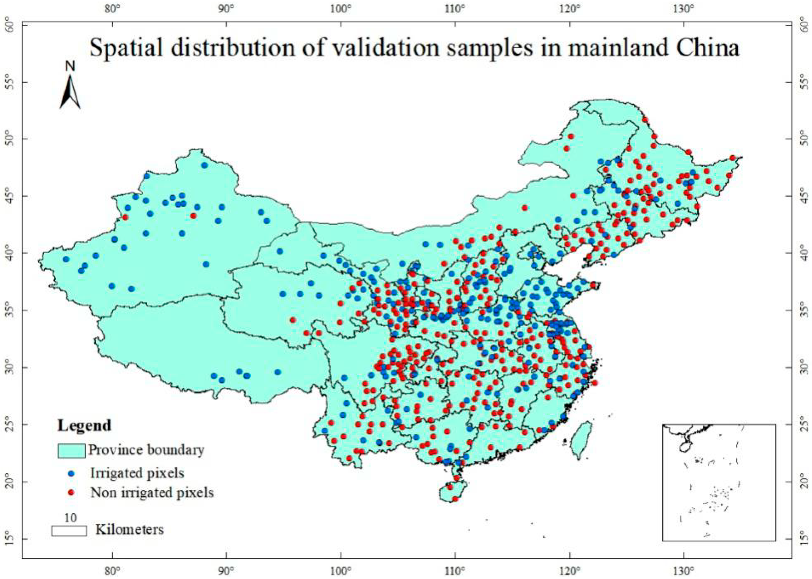
Figure 1. Study area and validation sites. The blue and red dots stand for the irrigated and non-irrigated sites, respectively.
Remotesensing 12 04181 g001
Figure 2. The LSWI difference (LSWIDiff) between non-irrigated (left) cropland pixels or irrigated (right) cropland pixels and their nearby forest pixels. (a) LSWIDiff of non-irrigated and irrigated cropland pixels at the investigated sites. (b) Histogram of LSWI values of non-irrigated cropland pixels, irrigated croplands pixels and nearby forests pixels in China; μ is the mean value of LSWI; the asterisk indicates a significant difference at the p < 0.01.
Remotesensing 12 04181 g002
Figure 3. The linear regression relationship between the (a) half of the Chinese provinces, (b) other half of the Chinese provinces LSWIDiff0 thresholds and the mean annual precipitation at the province level in mainland China.
Remotesensing 12 04181 g003
Figure 4. Comparison of irrigated areas in China as estimated by the proposed method and statistical data at the province (a) and prefecture (b) levels. The dotted line is the 1:1 line. The black dots in Figure 4a represent the 16 provinces used for building the relationship between LSWIDiff0 and mean annual precipitation, and the red dots correspond to the remaining 15 provinces used for verification. Statistical area refers to the irrigated area in a given administrative unit (province or prefecture) that were obtained from the statistical yearbooks.
Remotesensing 12 04181 g004
Figure 5. The location of irrigated areas in mainland China mapped in our study.
Remotesensing 12 04181 g005
Figure 6. Scatter plots comparing the irrigated area from our new map to FAO/UF and statistical data (a) and to Zhu’s map and IWMI data (b).
Remotesensing 12 04181 g006
Figure 7. Example of prefecture-level polygon maps in China aggregated from four irrigation maps: (a) irrigated regions calculated from our method, (b) irrigated regions calculated from FAO/UF map, (c) irrigated regions calculated from IWMI map, and (d) irrigated regions derived from Zhu’s dataset.
Remotesensing 12 04181 g007
Table 1. Province-level comparison of irrigated areas estimates from our method and statistical data for 2016.
ProvinceStatistical Area (Km2)Estimated Area (Km2)RPE
Anhui44,00335,556−19.20%
Beijing1374173626.37%
Chongqing687275579.97%
Fujian10,6173517−66.87%
Gansu13,0676209−52.49%
Guangdong17,71313,102−26.03%
Guangxi16,18811,877−26.63%
Guizhou10,6549462−11.19%
Hainan26402557−3.16%
Hebei44,48040,881−8.09%
Heilongjiang53,05269,98331.91%
Henan52,10665,32425.37%
Hubei28,99129,2560.91%
Hunan31,13318,907−39.27%
Jiangsu39,52527,253−31.05%
Jiangxi20,27718,150−10.49%
Jilin16,28820,76527.48%
Liaoning14,74026,17377.57%
Nei Mongol30,86933,4628.40%
Ningxia Hui50651684−66.75%
Qinghai19701636−16.96%
Shaanxi12,36810,794−12.73%
Shandong49,64449,018−1.26%
Shanghai18821477−21.55%
Shanxi14,60315,3415.05%
Sichuan27,35122,291−18.50%
Tianjin30891219−60.52%
Xinjiang 49,44936,549−26.09%
Xizang24785545123.76%
Yunnan17,5779218−47.56%
Zhejiang14,3227847−45.21%
Total654,387604,344−7.65%
Note: RPE (Relative predictive error): (Area estimated—Area statistics) / Area statistics × 100%.
Table 2. Overall accuracy of FAO/UF, IWMI, Zhu’s dataset, and our map of China.
FAO/UFIWMIZhu’s DatasetOur Map
Correctly classified pixels252361378380
Validation samples612612612612
Overall accuracy41.18%58.98%61.76%62.09%
Publisher’s Note: MDPI stays neutral with regard to jurisdictional claims in published maps and institutional affiliations.