Technical Note

A Machine Learning Approach for Mapping Forest Vegetation in Riparian Zones in an Atlantic Biome Environment Using Sentinel-2 Imagery

by
Danielle Elis Garcia Furuya
1,
João Alex Floriano Aguiar
2,
Nayara V. Estrabis
3,
Mayara Maezano Faita Pinheiro
1,
Michelle Taís Garcia Furuya
1,
Danillo Roberto Pereira
1,
Wesley Nunes Gonçalves
3,4,
Veraldo Liesenberg
5,
Jonathan Li
6,7,
José Marcato Junior
3,
Lucas Prado Osco
2 and
Ana Paula Marques Ramos
1,*
1
Post-Graduate Program of Environment and Regional Development, University of Western São Paulo, Rodovia Raposo Tavares, km 572, Bairro Limoeiro, SP 19067-175, Brazil
2
Faculty of Engineering and Architecture and Urbanism, University of Western São Paulo, Rodovia Raposo Tavares, km 572, Bairro Limoeiro, SP 19067-175, Brazil
3
Faculty of Engineering, Architecture and Urbanism and Geography, Federal University of Mato Grosso do Sul, Cidade Universitária, Av. Costa e Silva-Pioneiros, MS 79070-900, Brazil
4
Faculty of Computing, Federal University of Mato Grosso do Sul, Cidade Universitária, Av. Costa e Silva-Pioneiros, MS 79070-900, Brazil
5
Forest Engineering Department, Santa Catarina State University, Avenida Luiz de Camões 2090, Lages, SC 88520-000, Brazil
6
Department of Geography and Environmental Management, University of Waterloo, Waterloo, ON N2L 3G1, Canada
7
Department of Systems Design Engineering, University of Waterloo, Waterloo, ON N2L 3G1, Canada
*
Author to whom correspondence should be addressed.
Remote Sens. 2020, 12(24), 4086; https://doi.org/10.3390/rs12244086
Submission received: 13 October 2020 / Revised: 5 December 2020 / Accepted: 8 December 2020 / Published: 14 December 2020
(This article belongs to the Section AI Remote Sensing)

Abstract

:
Riparian zones consist of important environmental regions, specifically to maintain the quality of water resources. Accurately mapping forest vegetation in riparian zones is an important issue, since it may provide information about numerous surface processes that occur in these areas. Recently, machine learning algorithms have gained attention as an innovative approach to extract information from remote sensing imagery, including to support the mapping task of vegetation areas. Nonetheless, studies related to machine learning application for forest vegetation mapping in the riparian zones exclusively is still limited. Therefore, this paper presents a framework for forest vegetation mapping in riparian zones based on machine learning models using orbital multispectral images. A total of 14 Sentinel-2 images registered throughout the year, covering a large riparian zone of a portion of a wide river in the Pontal do Paranapanema region, São Paulo state, Brazil, was adopted as the dataset. This area is mainly composed of the Atlantic Biome vegetation, and it is near to the last primary fragment of its biome, being an important region from the environmental planning point of view. We compared the performance of multiple machine learning algorithms like decision tree (DT), random forest (RF), support vector machine (SVM), and normal Bayes (NB). We evaluated different dates and locations with all models. Our results demonstrated that the DT learner has, overall, the highest accuracy in this task. The DT algorithm also showed high accuracy when applied on different dates and in the riparian zone of another river. We conclude that the proposed approach is appropriated to accurately map forest vegetation in riparian zones, including temporal context.

Graphical Abstract

1. Introduction

Monitoring the spatial-temporal dynamics of land cover and use in riparian zones is essential to understand the numerous surface processes that can occur in these areas [1]. Deforestation and inadequate use are some of the most notorious problems in many environmentally fragile riparian zones. These regions have an important role in environmental conservation, providing multiple ecosystem services [2]. With the increasing loss worldwide of wetlands and riparian areas [2], an accurate mapping of forest vegetation is required to define strategies for both monitoring and conservation. Fine-scale mapping of forest vegetation in riparian zones may provide information to support different tasks, such as maintaining the quality of water resources. Riparian zones offer an ecological function essential to wildlife and human communities that are gathered around its proximities. In this regard, investigating methods that provide an accurate description of these forest fragments is a relevant scientific task.
Satellite imagery consists of a substantial source of information to map forests since they regularly register a wide geographic area and are particularly suited to support the changing detection tasks [3]. Moreover, satellite imagery is a potential solution for mapping land use at several cartographic scales [4]. An important orbital platform for monitoring these areas is the Sentinel-2. Offering multispectral images with 10–60 m spatial, 13 spectral bands, and 5-day temporal resolutions, Sentinel-2 images opened many opportunities to investigate the fine-scale mapping of vegetation, including inside the riparian zones. However, digital image classification is a task whose accuracy strongly depends on the availability of data and on the applied method used to perform it [5]. Image classification tasks were initially performed with conventional supervised methods like maximum likelihood, minimum distance, Mahalanobis distance, and others, as well as with unsupervised methods like K-means and isodatdo a [6]. Nonetheless, new approaches are required to aid this issue, especially because of the technological advances that permitted the construction of sensors able to acquire images with high spatial-spectral-temporal resolutions, thus, producing a large amount of data to be analyzed.
Machine learning (ML) techniques are a current and promising alternative to process remote sensing data [7] and are applied in many data processing and analysis tasks [8]. These learners can be used to model different sets-of-data using a robust approach [7,9]. Moreover, ML methods allow establishing non-parametric and nonlinear relationships between the independent variables and dependent variables (usually the target), resulting in overall better performance when compared to the conventional linear models [10]. Regardless, as no universal learner exists, multiple tests are needed for different types of applications.
Several approaches have been developed with ML and multispectral imagery for mapping the spatial distribution of vegetation areas. A study [11] investigated the performance of the random forest (RF) and support vector machine (SVM) algorithms for high-resolution multispectral imagery classification. These images were acquired with embedded sensors in an Unmanned Aerial Vehicle (UAV). The reliability of ML learners was also verified in the mapping task of invasive trees in riparian zones, also with UAV-imagery [12]. Adopting visible and near-infrared data, spectral and texture features were computed at various scales (10, 30, 45, 60), and the most relevant variable (or combination of variables) was identified with a supervised classification model based on the RF algorithm.
A recent study [13] pointed out that ML algorithms can be used for mapping vegetation areas, and they are especially applicable when training data consist of a large number of observations and covariates. More recently, another research [14] evaluated several multi-temporal Sentinel-2 images, making combinations of spectral bands and applying principal component analysis and tasseled cap transformations. They used it as input to four ML techniques (SVM, nearest neighbor—KNN, RF, and classification trees—CT), aiming to separate vegetation species. The best results were returned by SVM, but the authors pointed out that further work is needed to determine whether these results are replicable in other vegetation types and regions. Combinations of spectral bands from Sentinel-2 data were also tested [15] to evaluate the performance of the RF for mapping tree species on different dates, and obtained an averaged accuracy of 80%.
Although remote sensing images have proved their potential to support mapping tasks into different contexts, like land use and land cover, its application for forest vegetation mapping in the riparian zones exclusively is still limited. Up to our knowledge, few studies were conducted [11,12] in this manner, and they were mainly with UAV-imagery. UAV-imagery provides an important data source for many applications, like high-detailed vegetation maps, but it is worth mentioning that these platforms may not be attractive when wide geographic areas require to be mapped such as riparian zones in many tropical countries.
The use of machine learning methods with orbital data, like the free-available satellite images from Sentinel-2, can be a promissory strategy to map-wide areas using a low-cost approach. Sentinel-2 data has been evaluated with ML algorithms for mapping different types of vegetation [16,17], as other targets [18], and it was considered efficient in these studies. But, the knowledge about the capacity of current ML models to identify the spatial distribution of forest vegetation in riparian zones based on medium spatial resolution imagery is limited yet. A recent study [14] used Sentinel 2 imagery to map vegetation, but it is unclear whether these results can be replicated into other riparian zones.
To fulfill the aforementioned gap, we propose an easily reproducible framework to map forest vegetation in riparian zones, based on Sentinel-2 (MSI) multispectral images and processed by ML algorithms. We hypothesize that some machine learning algorithms may be more appropriate than others to potentially map forest-type in those areas with interference from seasonal changes. We then verified the -generalization capability of all trained models using images from different dates and geographic areas. The traditional classification and segmentation methods may not present a consistent accuracy or even provide the same robustness as a machine learning evaluation. In this sense, when monitoring these areas alongside different dates, governmental technical-agencies, and entities responsible for the forest management may adopt the proposed approach.

2. Materials and Methods

Our method was divided into four main stages (Figure 1). Initially, we performed the organization of a database composed of 14 multispectral Sentinel-2 imagery, acquired alongside a one-year-period, for the area of interest. These images were pre-processed to convert their original value into surface reflectance values [14].
We defined as a study area the riparian zone within 1 km distance from the Paraná river margin (Figure 2), and for the last step the riparian zone selected was within 1 km of another river, known as the Paranapanema. We manually labeled the features (forest and non-forest) in a geographical information system (GIS) environment and separated the data in both training and testing sets. We performed the detection of forest vegetation adopting different algorithms. The performance of the learners was compared against one another using classification evaluation metrics.

2.1. Study Area

Our study area was the riparian zone of the Paraná River (Figure 2) located in the state of São Paulo, Brazil. This region is known for the presence of one of the last original fragments of the Atlantic Biome in Brazil. This riparian zone has an area of 152.91 km² and 468.46 km of the perimeter, and the Paraná River is considered the most important river from this geographic region, dividing the states of São Paulo and Mato Grosso do Sul. The riparian zone is formed by both Cerrado (Brazilian Savanna) and Atlantic Forest biomes. This area is representative of most large rivers in our ecosystem, as it still possesses natural vegetation alongside deforestation, agricultural and urban environments within its area.

2.2. Image Preprocessing and Labeled Features

Our experiment considered a total of 14 Sentinel-2 images (Table 1). All scenes were available with little or without cloud interference alongside the riparian zone. Also, most of the cloud-cover was formed by thin clouds, which although may impact the algorithm’s performance, served as an additional challenge for the algorithm. A total of 13 Sentinel-2 images were acquired during June 2018 and June 2019 (one per month), and a scene from June 2020 was used to test the performance of the algorithms in a different period. Therefore, we worked with images representing all seasons of the year (summer, winter, autumn, and spring). Each scene was downloaded from the United States Geological Survey (USGS) EarthExplorer Platform. Sentinel-2 images are collected by its MSI sensor and available in Digital Number (DN), in 12-bit radiometric resolution, in both 10, 20, and 60 m resolutions. They were projected to the WGS-84 UTM 22 S zone system.
For all images, we performed the radiometric correction using the SNAP 7.1.0 software with the Sen2Cor Toolbox. It was necessary to minimize the atmospheric influences, and, for that, we adopted the recommendations listed in the Sentinel-2 User Handbook [19]. The SNAP tool finds the parameters for both radiometric and atmospheric corrections automatically. These values are calculated by default when the software reads the metadata file of each scene. In this regard, aerosol values corresponding to rural areas were adopted; and atmospheric conditions were defined to coincide with the time that the image was recorded. Ozone content in the atmosphere was also automatically defined. A correction using the Cirrus band (Band 10) was not performed since is not available for the 10 m bands at the moment [19]. We used the DSM (Digital Surface Model) option input for terrain correction. The remaining parameters were left at their respective default values.
For our experimental setup, we labeled the forest-type data as training and testing samples using a GIS tool. The collection of the labeled information was performed with help of a specialist in the area, alongside additional high-resolution imagery from other datasets and imaging (both orbital and aerial) performed within the riparian zone in the last years. Regarding different types of forest vegetation present in the riparian zone, we considered only the fragments formed by forest physiognomies from the Atlantic Biome and, in fewer proportions, Brazillian Savanna, commonly encountered in the area, and associated with wetlands. In this aspect, since this type of forest offers more protection to these fragile ecosystems than the arbustive or grassland-types, it was identified during the labeling process and incorporated in the analysis.
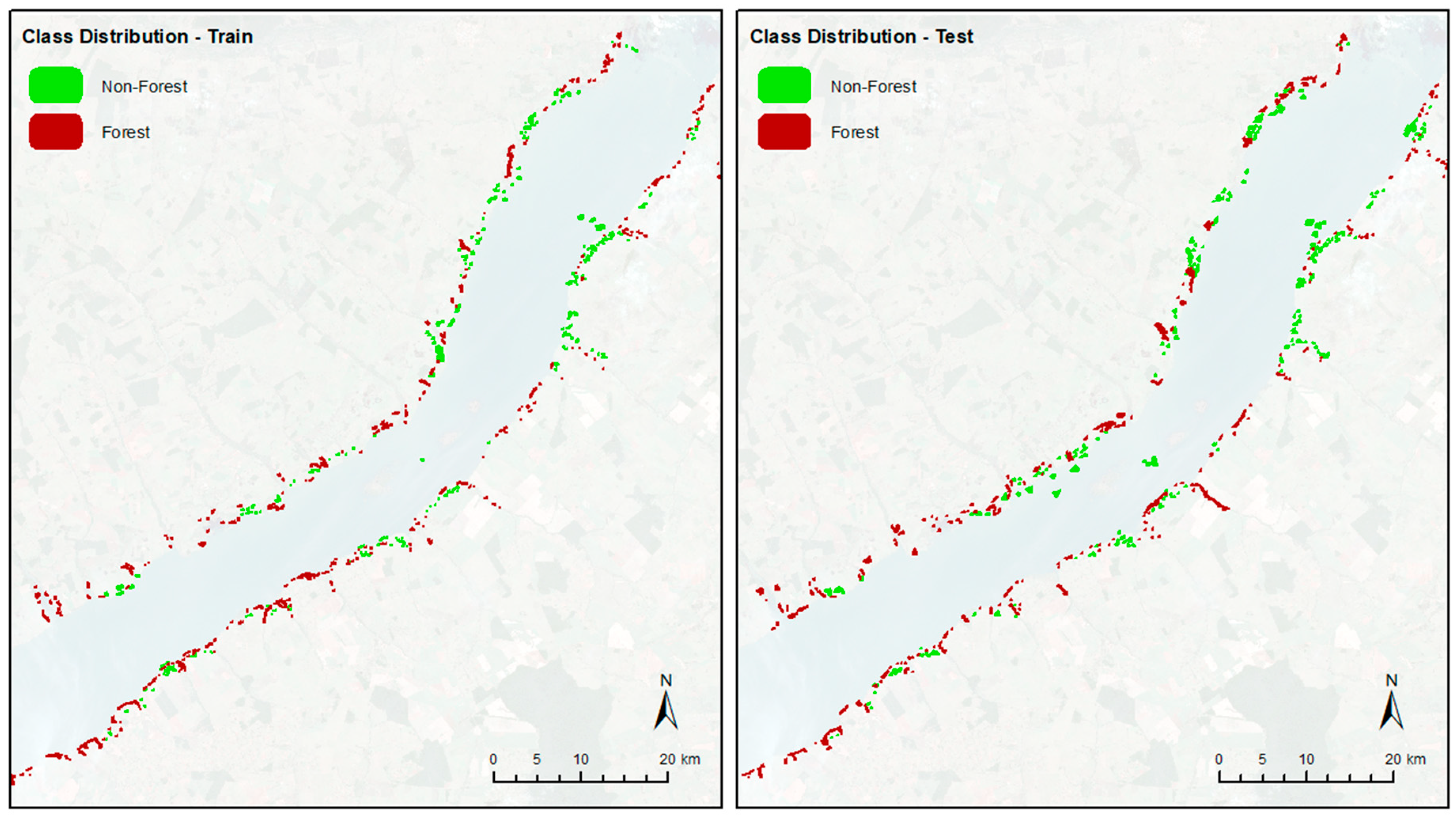
A total of 855 features (polygons) of forest-type vegetation and 855 features of non-forest vegetation (e.g., water, soil, grass, and other land covers) were annotated on Sentinel-2 images, resulting in a total of 1710 polygons with different sizes, occupying almost 3,322.3 ha. Details regarding these samples and their spatial distribution are presented in Table 2 and Figure 3 below. Although, by the proximity between polygons, it may seem that some of which are present in both subsets. However, this occurred only during the representation of small polygons in the figure scale, as both training and testing sets were composed of entirely different features. To investigate the performance of the machine learning algorithms in detecting forest vegetation, we used 50% of the dataset (polygon features) for training and 50% for testing the algorithms.
The sample size and quality of training data have generally had a large impact on the classification accuracy [20]. In this regard, we divided the dataset while ensuring that both training and testing sets contained similar sampling patterns, being representatives of all conditions observed in the area during labeling. This division was applied with the assistance of a widget incorporated in the Orange open-source software, and we integrated it with the sampling extraction method in the QGIS open-source software environment.

2.3. Machine Learning Algorithms

The open-source software Orfeo Toolbox 7.1.0 was used to apply and evaluate the performance of different ML models in classifying forest vegetation in the riparian zones using Sentinel-2 multispectral images. As stated, our dataset was composed of two classes: forest vegetation and non-forest vegetation, and it was used both training and testing the algorithms to ensure an adequate comparison among algorithms. We conducted a comparative study using five machine learning algorithms, including random forest [21], decision tree [22], support vector machine [23], and normal-gaussian Bayes [9].
The training and testing datasets were divided in the proportion of 50:50. The training set was then used to train and set up the hyperparameters of the chosen algorithms. In this sense, we divided the training set with the holdout method, using 10% of its data to validate it. After defining the best parameters for each model, we used the testing-set containing 50% of the original data, with samples not used during the training and validation process, to evaluate the real performance of our models. As explained by [24], the even division between samples is necessary to have a good balance between both sets. This ensures a reliable estimation of the models’ performance, as the imbalance between datasets may harm the predictions.
The fine-tuning process of all the algorithms was performed until no improvements in the F1-measure value were identified. The same dataset (training and testing) was adopted for all algorithms. The final configuration of the algorithms is in Table 3. Once the hyperparameters of each algorithm were defined, the testing dataset was used to verify its real performance. Metrics like global accuracy, F1-measure, precision, and recall were then adopted to evaluate them. These metrics were calculated considering the classification results of all of the labeled pixels in the testing-set. They also represent the average classification values between both classes.
Our experiment was set up to compare the performance of the machine learning models and determine the overall best classifier. This comparison was performed regarding only the spectral bands (blue, green, red, and near-infrared) from the 10 m spatial resolution images, as it provided more detailed samples. Additionally, we conducted tests to evaluate the generalization capability of all trained models using images from dates and geographic areas. The different proposed scenarios were related to a) evaluating different dates acquired during a one-year time interval (each image was evaluated individually by all of the machine learning models), and; b) applying the models in another riparian zone in an image from a different year of a different area; although from the same biome. Each image was then evaluated individually by all of the machine learning models.

3. Results

Table 4 shows the performance of the machine learning algorithms in the proposed task regarding the multiple dates of analysis for the riparian zone of the Paraná River (Figure 2). As previously explained, all models were trained on 50% of the sampling data and tested with the remaining 50% for a total of 14 Sentinel-2 imagery (Table 1) with the spectral bands’ number 2,3,4, and 8 (blue, green, red, and, near-infrared bands, respectively), with 10 m of spatial resolution.
To help illustrate the performance of ML algorithms in multiple dates (Table 4), we organized a box-plot indicating the F1-measure and other evaluation metrics of the applied models (Figure 4). Here, the overall results indicated that the performance of the algorithms, when considering all of the dates, were similar. However, DT outperformed slightly other ML models, since it returned the highest F1-measure value. The DT then is the most recommended approach in this regard. The NB model, however, may be useful since it is a simple model and does not require substantial processing costs.
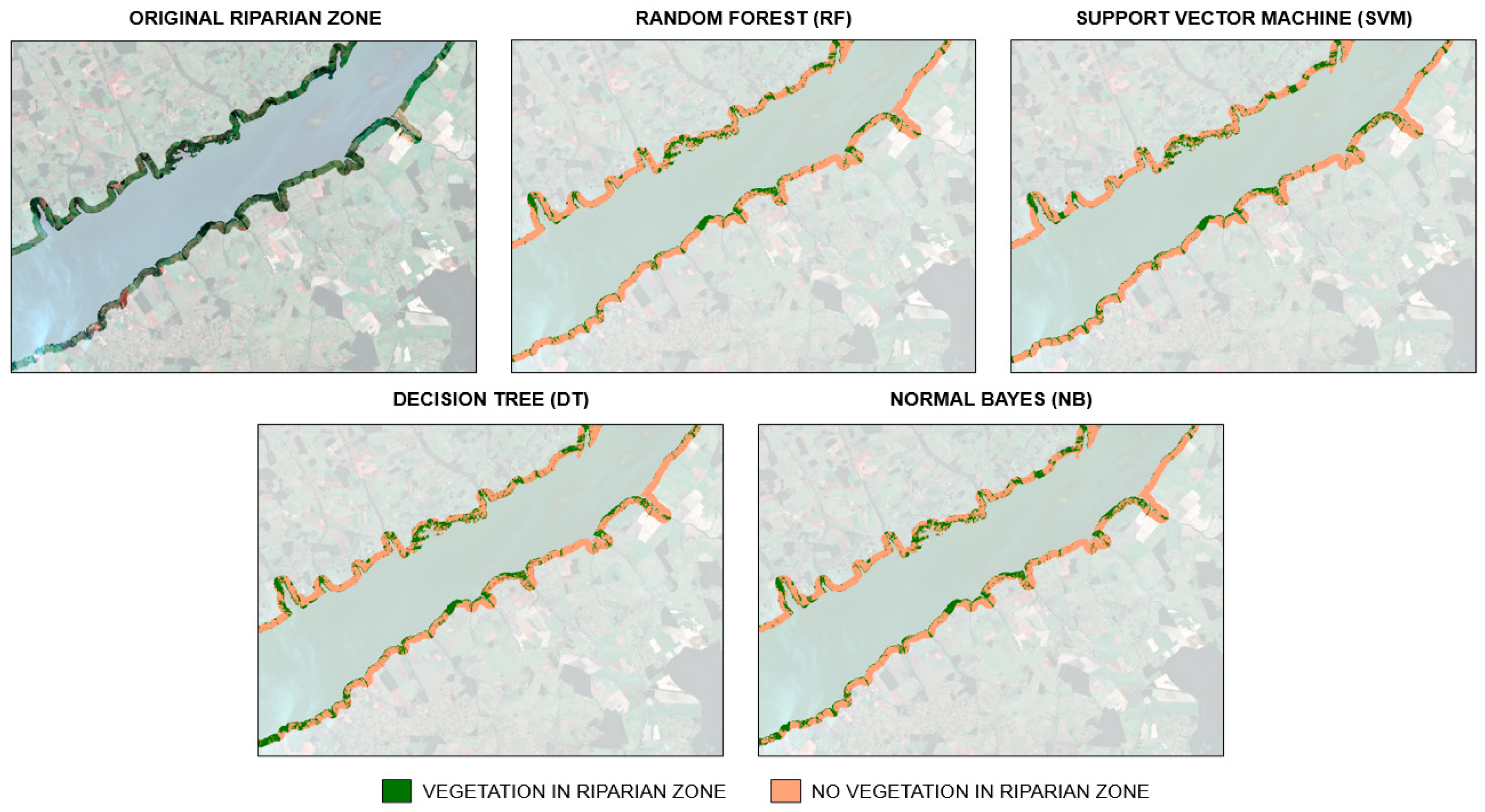
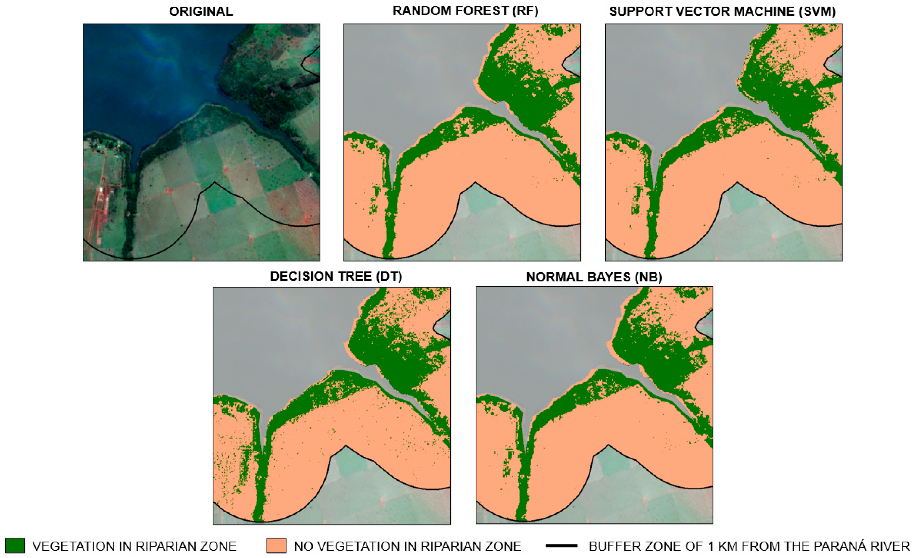
Figure 5 presents the qualitative results obtained with each tested ML algorithm using the image of 15 June 2019, since it returned the highest accuracy (F1-measure upper to 95%) compared to other dates (Table 4).
Although the five evaluated ML algorithms (Figure 5) can be assumed with similar performance visually, the quantitative analysis (Table 4) has demonstrated that the best learners in terms of kappa value were DT, NB, SVM, and RF, respectively. We noted that DT and NB techniques presented the same kappa value (95.20; see Table 4), but the NB, in general, had a slight increase in the Recall value compared to the DT (see Figure 4), which means that NB classified some non-forest areas as forest more than the DT algorithm. In this regard, the DT learner, while returning similar evaluation metrics as the other algorithms, returned better quali-quantitative results. Considering a forest management perspective, the false-positives (i.e., non-vegetation classified as vegetation) are more harmful than false-negatives.
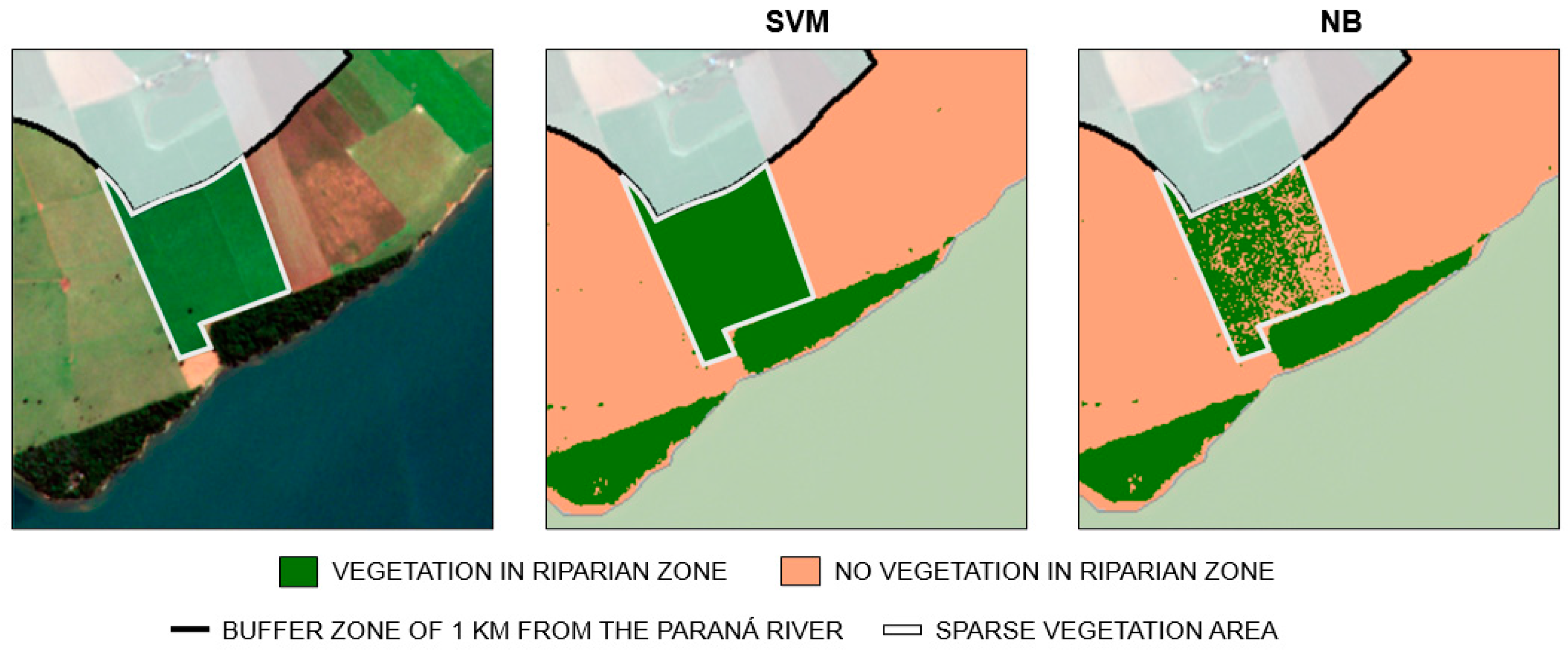
We verified that for some areas, the DT and RF algorithms were not affected by sparse vegetation characteristics (Figure 6) like the SVM and NB were (Figure 7). These areas present a higher contribution from soil brightness pixels and other types of vegetation covers that offer some potential challenges for the classification.
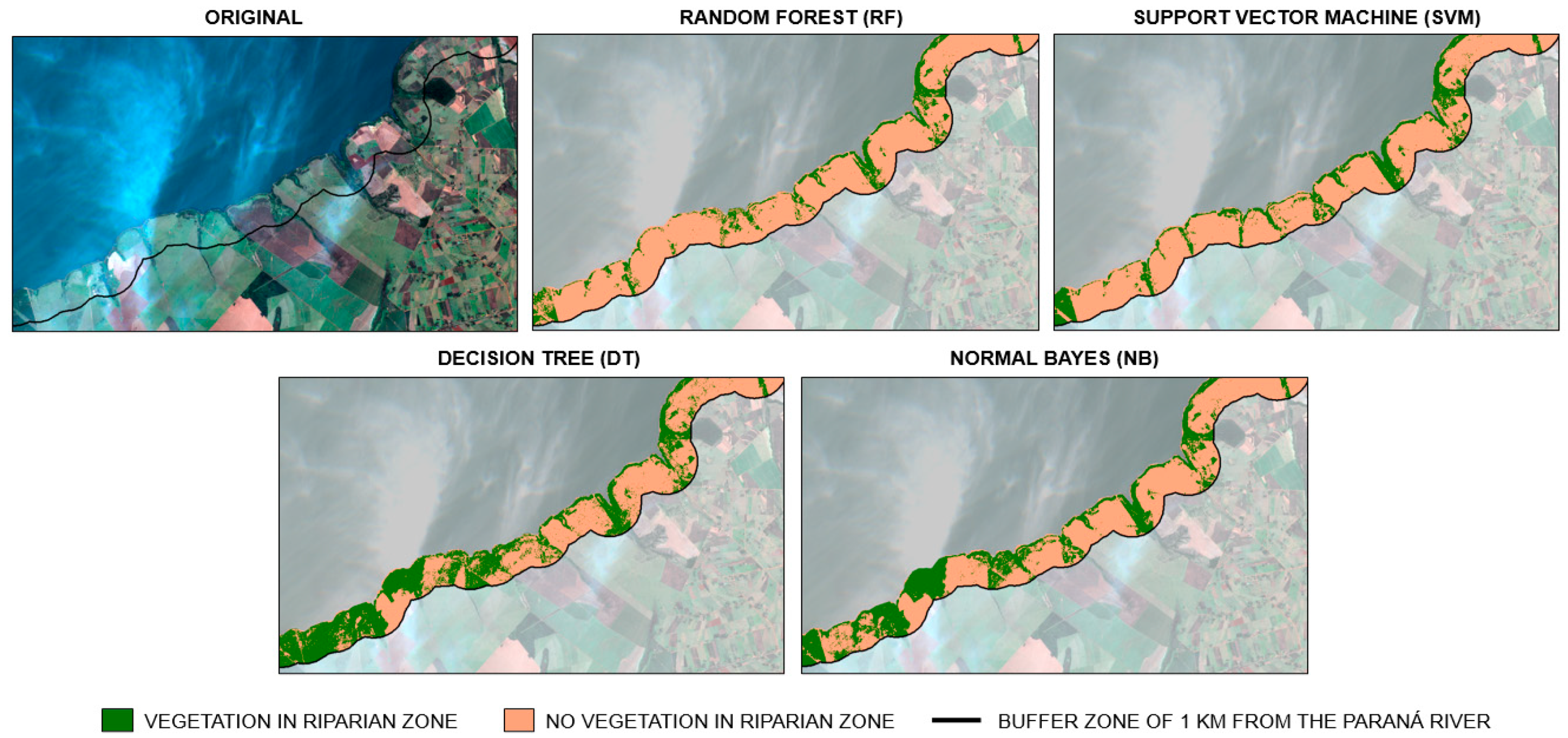
The algorithms also faced additional challenges in mapping forest vegetation in riparian zones, and negative examples are presented in Figure 8. This classification error possibly is due to the cloud cover interference that this part of the Sentinel-2 scene presented. The algorithms classified part of the clouded area over the water-body as vegetation. Nonetheless, the DT learner was still highly accurate in the proposed task when considering the land area contained within the riparian zone, as our training samples only considered these areas. Figure 9 shows a positive example in which the DT algorithm was successful in identifying forest vegetation in a complex environment.
Based on these observations (Figure 8 and Figure 9) and the results of the quantitative approach (Table 4), the DT was defined as the overall best technique among the evaluated models. To verify the generalization capability of the ML techniques, we performed additional tests with different dates in another riparian zone, but from the same biome. The generalization ability of a model refers to training it with images from a geographic area and testing its performance in other areas. This additional test was made with four algorithms (RF, SVM, DT, and NB). Therefore, the models, which were trained using images from the riparian zone of the Paraná River, were tested in the riparian zone located in the Paranapanema River. This river is located near one of the last largest fragments of primary vegetation from the Atlantic Biome, known as the Devil’s Mount. It is worth mentioning that we applied the four algorithms on two different dates in this area, considering the rainy summer and dry winter seasons. For that, we labeled a total of 147 features (polygons) representative of forest vegetation and 147 features of non-forest vegetation as data for testing the models, following the same criteria as the previous labeling. Table 5 shows the results, which returned high accuracies on all dates. Two representative dates of each year were considered in this analysis.
Considering the scene from December 2018, we verified that all algorithms present a decrease in performance in terms of kappa (Table 5). This is probably related to the cloud cover influence on this image, since, concerning June 2019, it presented 3,57 more times cloud cover (Table 1). The DT was the best algorithm among the evaluated models in terms of F1-measure, proving its generalization capability. To help ascertain the relationship between the spectral bands and the predictions, we present in Appendix A our decision tree models’ structure.

4. Discussion

The approach presented here is appropriated to map forest vegetation using satellite multispectral imagery of medium-spatial resolution. Our particular interest was to investigate the potential of machine learning algorithms and measure their variation in performance when applied to Sentinel-2 images for this task in riparian zones. The main advantage of this procedure is that free-available orbital images are used as the dataset, consisting of a low-cost method to support different environmental tasks, like monitoring of landscapes and forest management. In this regard, environmental practices could benefit from it, and future researches could be guided properly in terms of data and temporal analysis.
Studies [4,15] have shown that ML techniques are an efficient approach to map different land use and land cover classes, including forest vegetation, and our trials demonstrated that some algorithms can perform this task with higher accuracy than the others. The DT algorithm has been characterized as a simple and fast model for many applications in the remote sensing domain [25,26]. It was already characterized as more accurate, has less error rate, and is easier to apply when compared to other known methods in similar research [27]. In our investigation, the DT algorithm achieved satisfactory results both at different dates and locations. Visually, this algorithm returned better results than others, moreover in areas that were not sampled. It also returned some variation in its accuracy when regarding different dates, although fewer than most of the others (Figure 4).
The performance of the machine learning algorithms in our research was similar to those encountered in other studies [14,28,29]. In subtropical forest areas, a study [30] was able to obtain a kappa coefficient (k) of 0.74 for the RF algorithm using WorldView-2 imagery. The authors also improved their classification by adopting LiDAR data, resulting in metrics similar to ours. However, it should be highlighted that both WorldView-2 images and LiDAR surveying are expensive approaches, differently from our proposed method herein that is free. Others studies also presented high performances in separating forest areas from other types of land covers, like detecting natural forest in Sentinel-2 images with the RF algorithm [31], and separating forest healthy vegetation from damaged vegetation using, in this approach, deep neural networks, and returning 92% accuracy [32]. We can observe that, in our case of study, the obtained results are similar in terms of accuracy value, even though when a deep learning strategy is adopted, like in [32].
The strategy of adopting images from different dates was also encountered in related studies [14,15]. The temporal resolution is important and has been regarded as a more relevant feature than the spectral and spatial resolution when considering vegetation classification tasks [33]. In a recent study [14], the overall best accuracies were obtained during the winter season, something also observed in our approach. The winter period in the riparian region investigated presents less atmospheric interference than the other periods. However, the spectral behavior from the tree fragments may vary, as some species reduce the number of leaves during this season. Regardless, the main aspect remains the presence of cloud interference, and that may explain the differences in accuracy of other seasons (Table 4), such as summer, in which most of the images possess some sort of atmospheric interference.
Regarding vegetation phenology, few studies, to the best of our knowledge, evaluated different subclasses of forest-type with multispectral medium-spatial resolution remote sensing imagery and machine learning algorithms. Recently, in [14], the authors used multi-temporal Sentinel-2 images to capture the phenological differences between vegetation classes. This study implemented a 60:40 division between training and testing samples and determined that the classification of different phenologies was better with the SVM (74% accuracy) and NN (72% accuracy) models, returning superior results when compared against other algorithms, like RF (65% accuracy). Nonetheless, it is still difficult to evaluate different phenologies in medium-spatial resolution imagery, and future research could investigate the performance of these methods to map subtypes of forest in riparian zones by implementing other types of data to feed their models.
Another important observation to be made is related to the generalization capability of the machine learning algorithms. These algorithms, unlike other types of traditional classification models, such as Maximum Likelihood, can improve their performance and learning capability when considering more and different informative data for training [7,9]. In this aspect, it is possible to adopt the models for different scenarios, providing that enough characteristics are available for learning during its training phase. In our study, by implementing a 50:50 division between both training and testing samples, we demonstrated that most of the algorithms returned satisfactory performances and that most of them can be applied for different seasons throughout the year. The results obtained in a different riparian zone (Table 5) help to demonstrate the applicability of these models.
In short, our model was trained with data from one riparian zone, related to the Paraná river, and was able to map the forest vegetation considering different conditions (dates and areas) in the riparian zone of another river, known as the Paranapanema. This last experiment showed that the DT model, as well as the others to some extent, can be applied to different sites. As shown in Table 5, the worst results obtained in this area occurred during the rainy season (which happens from December to January in this region). As previously explained, the reduction in these dates could be explained mainly because the rainy season impacts the spectral response of vegetation [5], as well as promotes different atmospheric conditions that could also affect it such as the increase in cloud cover.
In a general sense, the machine learning algorithms investigated in this study can be considered a robust approach to classify forest-areas in multispectral imagery across seasonal periods. As we only implemented images from the Sentinel-2 sensor, this approach is suitable for low-cost classification models that intend to monitor areas like the ones adopted here. Nonetheless, other types of data may help in improving the accuracy in dates that did not return similar accuracies (Table 4) as the remaining pattern from the rest of the year. One study [31] indicated that a combination of texture metrics from Sentinel-2, seasonality metrics from Landsat time-series, and topography metrics from the SRTM digital elevation model are important features to be incorporated and fed to these models, helping to improve their overall performances in closed canopy natural forest classification.

5. Conclusions

Here, we evaluated the performance of multiple machine learning models for mapping forest vegetation in riparian zones using multispectral images collected by an orbital sensor, embedded in the Sentinel-2 platform. Our approach demonstrated that the DT algorithm presented better overall accuracy in the aforementioned challenge. However, all tested methods returned high accuracies, which could also be considered appropriate to perform this task. As a contribution, we concluded that the DT algorithm can be used in different images and geographic areas throughout the year, and this approach may be implemented into other forest vegetation mapping tasks. Our framework is appropriate to accurately map forest-type in riparian zones and future research may benefit from the information presented here.

Author Contributions

Conceptualization, A.P.M.R., and L.P.O.; methodology, D.E.G.F., and N.V.E.; formal analysis, D.E.G.F.; writing—original draft preparation, D.E.G.F.; writing—review and editing, A.P.M.R., L.P.O., N.V.E., M.M.F.P., M.T.G.F., J.A.F.A., V.L., D.R.P., W.N.G., J.L., J.M.J.; supervision, A.P.M.R.; project administration, A.P.M.R., L.P.O. All authors have read and agreed to the published version of the manuscript.

Funding

This research was funded by the National Council for Scientific and Technological Development (CNPq), grant number 303559/2019-5, 433783/2018-4, 310517/2020-6, and 313887/2018-7. V. Liesenberg is supported by FAPESC (2017TR1762).

Acknowledgments

The authors acknowledge the support of UFMS (Federal University of Mato Grosso do Sul), and CAPES (Coordination for the Improvement of Higher Education Personnel - Finance code 001).

Conflicts of Interest

The authors declare no conflict of interest. The funders had no role in the design of the study; in the collection, analyses, or interpretation of data; in the writing of the manuscript, or in the decision to publish the results.

Appendix A

To help ascertain the relationship between the spectral bands and the predictions, we present in this section our decision tree models’ structure in text form. This structure can be accessed via the link < https://github.com/OscoLP/remotesensing-12-04086_DecisionTree/blob/main/Structure >, with additional information regarding it. The model was constructed with training samples from different dates, collected at the riparian zone of the Parana river. The presented structure is from the pruned tree model, with a total of 394 leaves and 787 nodes.

References

  1. Midekisa, A.; Holl, F.; Savory, D.J.; Andrade-Pacheco, R.; Gething, P.W.; Bennett, A.; Sturrock, H.J.W. Mapping land cover change over continental Africa using Landsat and Google Earth Engine cloud computing. PLoS ONE 2017, 12, e0184926. [Google Scholar] [CrossRef] [PubMed]
  2. Chignell, S.M.; Luizza, M.W.; Skach, S.; Young, N.E.; Evangelista, P.H. An integrative modeling approach to mapping wetlands and riparian areas in a heterogeneous Rocky Mountain watershed. Remote Sens. Ecol. Conserv. 2017, 4, 150–165. [Google Scholar] [CrossRef] [Green Version]
  3. Lawley, V.; Lewis, M.; Clarke, K.; Ostendorf, B. Site-based and remote sensing methods for monitoring indicators of vegetation condition: An Australian review. Ecol. Indic. 2016, 60, 1273–1283. [Google Scholar] [CrossRef] [Green Version]
  4. Ba, A.; Laslier, M.; Dufour, S.; Hubert-Moy, L. Riparian trees genera identification based on leaf-on/leaf-off airborne laser scanner data and machine learning classifiers in western France. Int. J. Remote Sens. 2019, 41, 1645–1667. [Google Scholar] [CrossRef]
  5. Jensen, J.R. Remote Sensing of Environment: An Earth Resource Perspective, 2nd ed.; Pearson New International Edition: Harlow, UK, 2014; p. 619. [Google Scholar]
  6. Richards, J.A. Remote Sensing Digital Image Analysis, 5th ed.; Springer Verlag: New York, NY, USA, 2013; p. 503. [Google Scholar] [CrossRef]
  7. Ball, J.E.; Anderson, D.T.; Chan, C.S. Comprehensive survey of deep learning in remote sensing: Theories tools and challenges for the community. J. Appl. Remote Sens. 2017, 11, 042609. [Google Scholar] [CrossRef] [Green Version]
  8. Cheng, X.; Zheng, Y.; Zhang, J.; Yang, Z. Multitask Multisource Deep Correlation Filter for Remote Sensing Data Fusion. IEEE J. Sel. Top. Appl. Earth Obs. Remote Sens. 2020, 13, 3723–3734. [Google Scholar] [CrossRef]
  9. Mitchell, T.M. Machine Learning, 1st ed.; McGraw-Hill, Inc.: New York, NY, USA, 1997. [Google Scholar]
  10. Feng, P.; Wang, B.; Liu, D.L.; Yu, Q. Machine learning-based integration of remotely-sensed drought factors can improve the estimation of agricultural drought in South-Eastern Australia. Agric. Syst. 2019, 173, 303–316. [Google Scholar] [CrossRef]
  11. De Luca, G.; Silva, J.M.N.; Cerasoli, S.; Araújo, J.; Campos, J.; Di Fazio, S.; Modica, G. Object-Based Land Cover Classification of Cork Oak Woodlands using UAV Imagery and Orfeo ToolBox. Remote Sens. 2019, 11, 1238. [Google Scholar] [CrossRef] [Green Version]
  12. Michez, A.; Piégay, H.; Jonathan, L.; Claessens, H.; Lejeune, P. Mapping of riparian invasive species with supervised classification of Unmanned Aerial System (UAS) imagery. Int. J. Appl. Earth Obs. Geoinf. 2016, 44, 88–94. [Google Scholar] [CrossRef]
  13. Hengl, T.; Walsh, M.G.; Sanderman, J.; Wheeler, I.; Harrison, S.P.; Prentice, I.C. Global mapping of potential natural vegetation: An assessment of machine learning algorithms for estimating land potential. PeerJ 2018, 6, e5457. [Google Scholar] [CrossRef] [Green Version]
  14. MacIntyre, P.; Van Niekerk, A.; Mucina, L. Efficacy of multi-season Sentinel-2 imagery for compositional vegetation classification. Int. J. Appl. Earth Obs. 2020, 85, 101980. [Google Scholar] [CrossRef]
  15. Persson, M.; Lindberg, E.; Reese, H. Tree species classification with multi-temporal Sentinel-2 data. Remote Sens. 2018, 10, 1794. [Google Scholar] [CrossRef] [Green Version]
  16. Cai, Y.; Zhang, M.; Lin, H. Estimating the Urban Fractional Vegetation Cover Using an Object-Based Mixture Analysis Method and Sentinel-2 MSI Imagery. IEEE J. Sel. Top. Appl. Earth Obs. Remote Sens. 2020, 13, 341–350. [Google Scholar] [CrossRef]
  17. Feng, S.; Zhao, J.-J.; Liu, T.; Zhang, H.; Zhang, Z.; Guo, X. Crop Type Identification and Mapping Using Machine Learning Algorithms and Sentinel-2 Time Series Data. IEEE J. Sel. Top. Appl. Earth Obs. Remote Sens. 2019, 12, 3295–3306. [Google Scholar] [CrossRef]
  18. Balcik, F.B.; Senel, G.; Goksel, C. Object-Based Classification of Greenhouses Using Sentinel-2 MSI and SPOT-7 Images: A Case Study from Anamur (Mersin), Turkey. IEEE J. Sel. Top. Appl. Earth Obs. Remote Sens. 2020, 13, 2769–2777. [Google Scholar] [CrossRef]
  19. Sentinel; European Space Agency (ESA). Sentinel-2 User Handbook; ESA Standard Document; ESA: Paris, France, 2015. Available online: https://sentinels.copernicus.eu/web/sentinel/user-guides/document-library/-/asset_publisher/xlslt4309D5h/content/sentinel-2-user-handbook (accessed on 9 December 2020).
  20. Maxwell, A.E.; Warner, T.A.; Fang, F. Implementation of machine-learning classification in remote sensing: An applied review. Int. J. Remote Sens. 2018, 39, 2784–2817. [Google Scholar] [CrossRef] [Green Version]
  21. Breiman, L. Random forests. Mach. Learn. 2001, 45, 5–32. [Google Scholar] [CrossRef] [Green Version]
  22. Breiman, L.; Friedman, J.H.; Olshen, R.A.; Stone, C.J. Classification and Regression Trees; Chapman and Hall/CRC Press: Boca Raton, FL, USA, 1984. [Google Scholar]
  23. Mountrakis, G.; Im, J.; Ogole, C. Support vector machines in remote sensing: A review. ISPRS J. Photogramm. Remote Sens. 2011, 66, 247–259. [Google Scholar] [CrossRef]
  24. Xu, Y.; Goodacre, R. On Splitting Training and Validation Set: A Comparative Study of Cross-Validation, Bootstrap, and Systematic Sampling for Estimating the Generalization Performance of Supervised Learning. J. Anal. Test. 2018, 2, 249–262. [Google Scholar] [CrossRef] [Green Version]
  25. Sharma, H.; Kumar, S. A survey on decision tree algorithms of classification in data mining. Int. J. Sci. Res. 2016, 5, 2094–2097. [Google Scholar]
  26. Jadhav, S.D.; Channe, H.P. Comparative Study of K-NN Naive Bayes and Decision Tree Classification Techniques. Int. J. Sci. Res. 2016, 5, 1842–1845. [Google Scholar] [CrossRef]
  27. Immitzer, M.; Vuolo, F.; Atzberger, C. First experience with sentinel-2 data for crop and tree species classifications in Central Europe. Remote Sens. 2016, 8, 166. [Google Scholar] [CrossRef]
  28. Brovelli, M.A.; Sun, Y.; Yordanov, V. Monitoring forest change in the amazon using multi-temporal remote sensing data and machine learning classification on Google Earth Engine. ISPRS Int. J. Geo-Inf. 2020, 9, 580. [Google Scholar] [CrossRef]
  29. Haq, M.A.; Rahaman, G.; Baral, P.; Ghosh, A. Deep Learning Based Supervised Image Classification Using UAV Images for Forest Areas Classification. J. Indian Soc. Remote Sens. 2020, 3, 1–6. [Google Scholar] [CrossRef]
  30. Sothe, C.; De Almeida, C.M.; Schimalski, M.B.; Liesenberg, V.; La Rosa, L.E.C.; Castro, J.D.B.; Feitosa, R.Q. A comparison of machine and deep-learning algorithms applied to multisource data for a subtropical forest area classification. Int. J. Remote Sens. 2020, 41, 1943–1969. [Google Scholar] [CrossRef]
  31. Koskikala, J.; Kukkonen, M.; Käyhkö, N. Mapping natural forest remnants with multi-source and multi-temporal remote sensing data for more informed management of global biodiversity hotspots. Remote Sens. 2020, 12, 1429. [Google Scholar] [CrossRef]
  32. Hamdi, Z.M.; Brandmeier, M.; Straub, C. Forest damage assessment using deep learning on high resolution remote sensing data. Remote Sens. 2019, 11, 1976. [Google Scholar] [CrossRef] [Green Version]
  33. Rapinel, S.; Mony, C.; Lecoq, L.; Clément, B.; Thomas, A.; Hubert-Moy, L. Evaluation of Sentinel-2 time-series for mapping floodplain grassland plant communities. Remote Sens. Environ. 2019, 223, 115–129. [Google Scholar] [CrossRef]
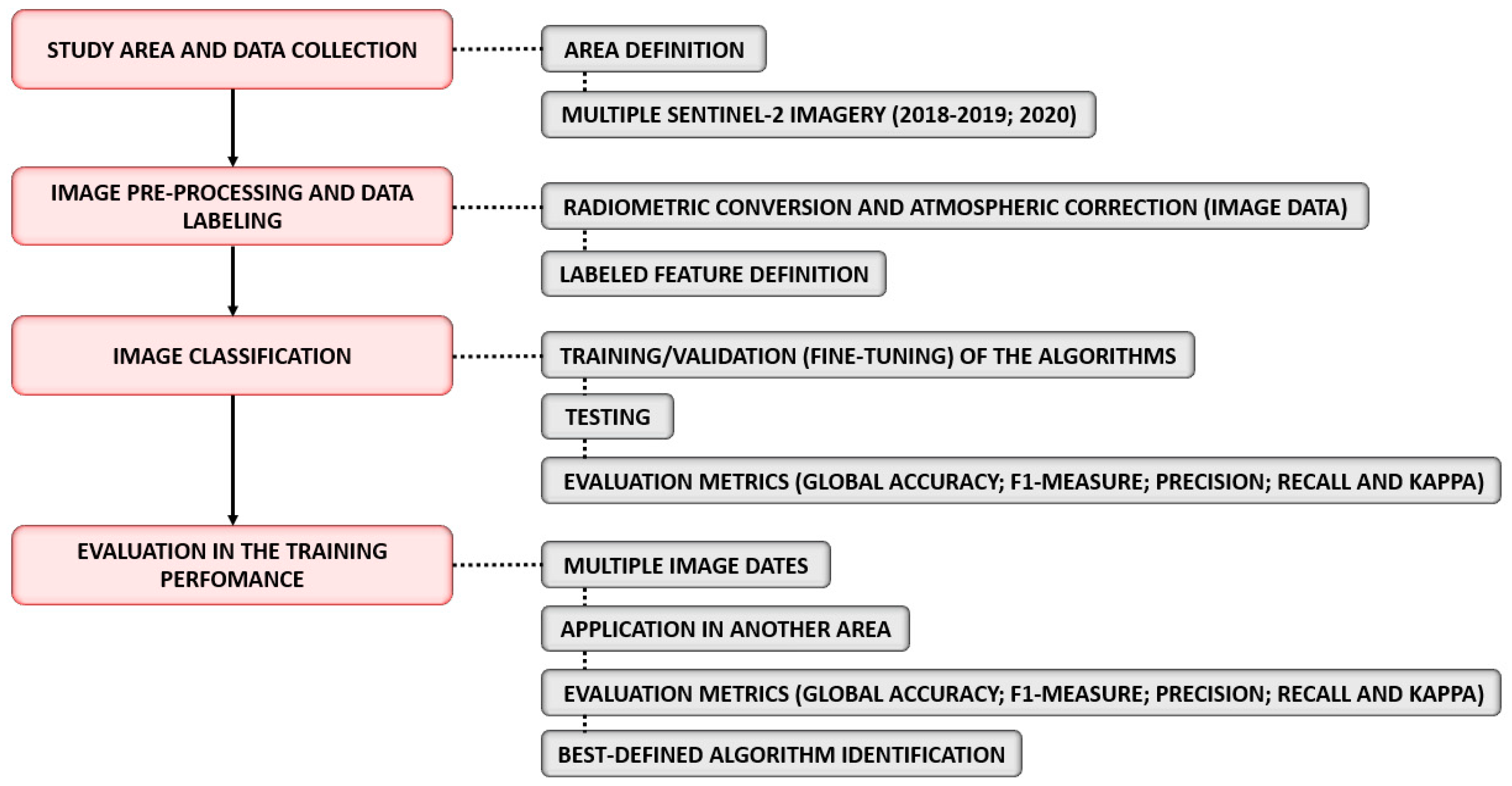
Figure 1. Workflow describing the main stages of the proposed method.
Remotesensing 12 04086 g001
Figure 2. Study area and an example of 1 km of the riparian zone.
Remotesensing 12 04086 g002
Figure 3. Spatial distribution of the complete dataset used in the Parana river area exemplifying the different classes.
Remotesensing 12 04086 g003
Figure 4. Box-plot representing the overall accuracies of the algorithms when considering multiple dates on its evaluation.
Remotesensing 12 04086 g004
Figure 5. Results of the image classifications of each algorithm.
Remotesensing 12 04086 g005
Figure 6. Examples of the classification of the DT and RF algorithms in an area of sparse vegetation.
Remotesensing 12 04086 g006
Figure 7. Examples of the classification of the SVM and NB algorithms in an area of sparse vegetation.
Remotesensing 12 04086 g007
Figure 8. Examples of the classification results obtained with the algorithms using the Sentinel-2 image with the partially-cloudy area.
Remotesensing 12 04086 g008
Figure 9. Examples of the classification results obtained with the algorithms using the Sentinel-2 image from without cloud cover.
Remotesensing 12 04086 g009
Table 1. Information regarding the 14 Sentinel-2 images used in this study.
DateSeason in the South Hemisphere
20 June 2018Autumn
20 July 2018Winter
29 August 2018Winter
23 September 2018Spring
28 October 2018Spring
27 November 2018Spring
02 December 2018Spring
31 January 2019Summer
10 February 2019Summer
22 March 2019Autumn
26 April 2019Autumn
21 May 2019Autumn
15 June 2019Autumn
24 June 2020Winter
Table 2. Description of the training, validation, and testing sets of the dataset.
DatasetNumber of Samples (Features—Polygon)Area (ha)Number of Pixels
Training (Forest)430839.008,390,000
Training (Non-Forest)425679.056,790,500
Testing (Forest)447893.408,934,000
Testing (Non-Forest)408910.859,108,500
Table 3. ML algorithms adopted to classify forest vegetation in riparian zones.
AlgorithmHyperparameters
RFMaximum depth of the tree = 5
Minimum number of samples in each node = 10
Termination criteria for regression tree = 0
Cluster possible values of a categorical variable into k <= clusters to find a suboptimal split = 10
Size of the randomly selected subset of features at each tree node = 0
Maximum number of trees in the forest = 100
Sufficient accuracy = 0.01
SVMSVM Kernel Type = Linear
SVM Model Type = C support vector classification
Cost parameter C = 1
Cost parameter Nu = 0.5
Parameters optimization = Off
Probability estimation = Off
DTMaximum depth of the tree = 10
Minimum number of samples in each node = 10
Termination criteria for regression tree = 0.01
Cluster possible values of a categorical variable into k <= cat clusters to find a suboptimal split = 10
NBThe algorithm has no parameters for changing
Table 4. Performance evaluation applying the trained model on all dates with different models.
Algorithm—DateAccuracy (%)F1-Measure (%)Precision (%)Recall (%)Kappa (%)
RF—June 201886.1084.3573.6498.7072.30
RF—July 201886.1084.3573.6498.7072.30
RF—August 201896.5589.5582.5596.5575.10
RF—September 201897.0790.7484.4197.0775.70
RF—October 201894.7994.6089.8999.8489.60
RF—November 201893.0192.6386.3999.8386.00
RF—December 201888.3887.2578.2298.6476.80
RF—January 201956.2938.6727.1067.4413.40
RF—February 201980.2576.2962.5197.8560.70
RF—March 201992.9293.9295.6990.8785.80
RF—April 201997.1397.1997.9096.5094.20
RF—May 201986.2885.3978.8693.1072.60
RF—June 201995.4295.3893.0897.8090.80
RF—June 202067.4858.2244.5783.9135.50
SVM—June 201890.3889.6281.7699.1680.80
SVM—July 201888.0282.7777.5288.0281.55
SVM—August 201885.2581.6778.1085.2580.77
SVM—September 201886.3984.5973.4899.6572.90
SVM—October 201896.7996.7694.1999.4693.60
SVM—November 201893.6093.4689.8997.3287.20
SVM—December 201891.8991.7088.1895.5283.80
SVM—January 201984.6183.2175.0393.3969.30
SVM—February 201980.9378.3067.6892.8962.00
SVM—March 201991.2791.7495.3288.4182.50
SVM—April 201995.8195.9096.4695.3591.60
SVM—May 201993.0392.8789.3796.6686.10
SVM—June 201995.8795.9295.5096.3391.70
SVM—June 202082.9480.0867.4798.4866.00
DT—June 201892.2792.6495.7589.7384.50
DT—July 201894.8394.8192.9196.7989.70
DT—August 201891.7291.4987.5895.7683.50
DT—September 201892.4192.0986.8498.0284.90
DT—October 201892.6192.6291.1894.1185.20
DT—November 201889.2589.2287.4991.0278.50
DT—December 201887.6087.5585.7389.4475.20
DT—January 201946.2045.7044.5346.93−07.50
DT—February 201980.7881.1781.5080.8461.50
DT—March 201991.6392.1796.9087.8783.20
DT—April 201995.7495.9198.2993.6591.50
DT—May 201968.2674.7792.5062.7436.00
DT—June 201997.6197.6697.8797.4495.20
DT—June 202067.9575.0794.9462.0835.30
NB—June 201896.7496.7194.4599.0993.50
NB—July 201894.2293.9593.6994.2291.25
NB—August 201895.5894.9094.2295.5892.58
NB—September 201890.4989.6981.3599.9381.00
NB—October 201878.9581.2489.6774.2657.70
NB—November 201861.7068.7482.8558.7422.80
NB—December 201870.9375.4187.7066.1441.50
NB—January 201976.6978.0981.7374.7653.30
NB—February 201980.7582.5889.7776.4661.40
NB—March 201992.8893.2496.5590.1585.70
NB—April 201996.3096.4297.9994.9192.60
NB—May 201994.1694.2694.3794.1688.30
NB—June 201997.6297.6698.0497.2995.20
NB—June 202086.6187.9195.7881.2473.10
Table 5. Performance evaluation of four algorithms applying the trained model on different dates in the Paranapanema River.
Algorithm—DateAccuracy (%)F1-Measure (%)Precision (%)Recall (%)Kappa
RF—December 201896.1297.6596.7198.6186.50
RF—June 201998.6799.2199.5798.8595.10
SVM—December 201899.0899.4498.9299.9896.70
SVM—June 201998.6899.2199.8198.6295.10
DT—December 201895.6597.4298.4396.4383.60
DT—June 201999.0499.4299.8798.9996.50
NB—December 201894.3996.7198.8894.6377.70
NB—June 201998.9099.3599.6799.0396.00
Publisher’s Note: MDPI stays neutral with regard to jurisdictional claims in published maps and institutional affiliations.