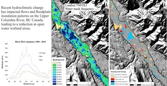
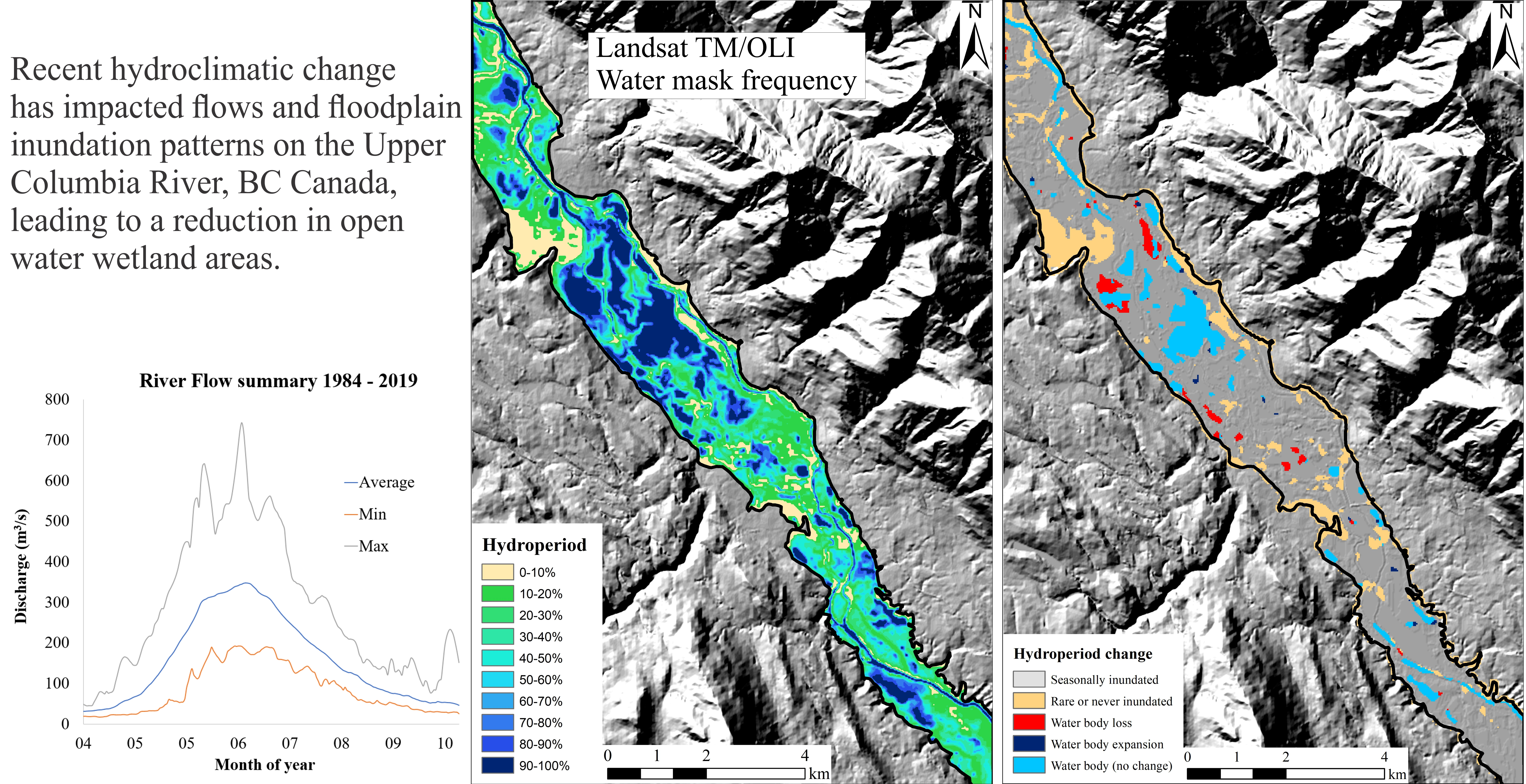
Wetland Hydroperiod Change Along the Upper Columbia River Floodplain, Canada, 1984 to 2019

 ,
,  and
and
Abstract
1. Introduction
1.1. Floodplain Wetland Vulnerability
1.2. Remote Sensing of Water Extent and Hydroperiod
1.3. Objectives
2. Materials and Methods
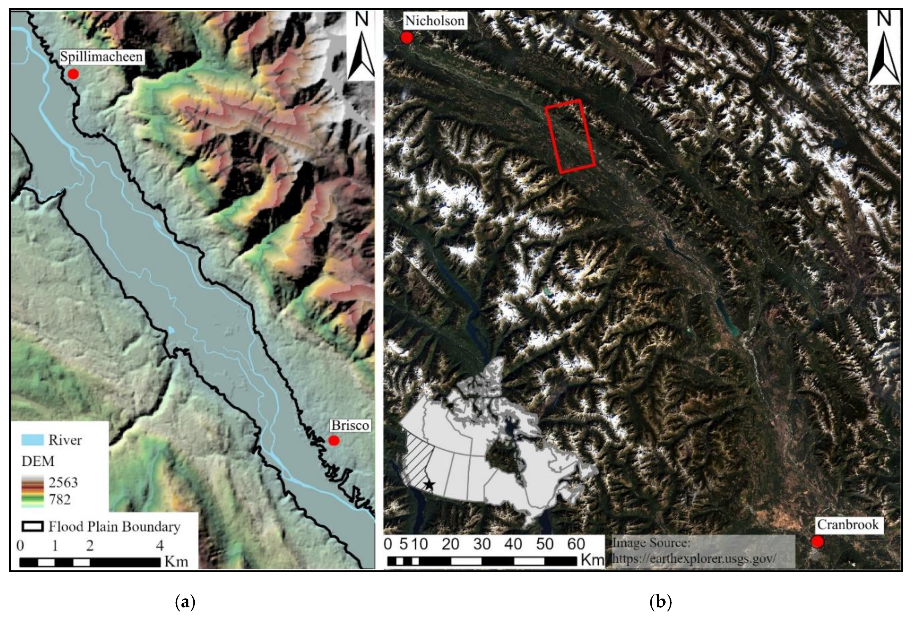
2.1. Study Area
2.2. Data Sources
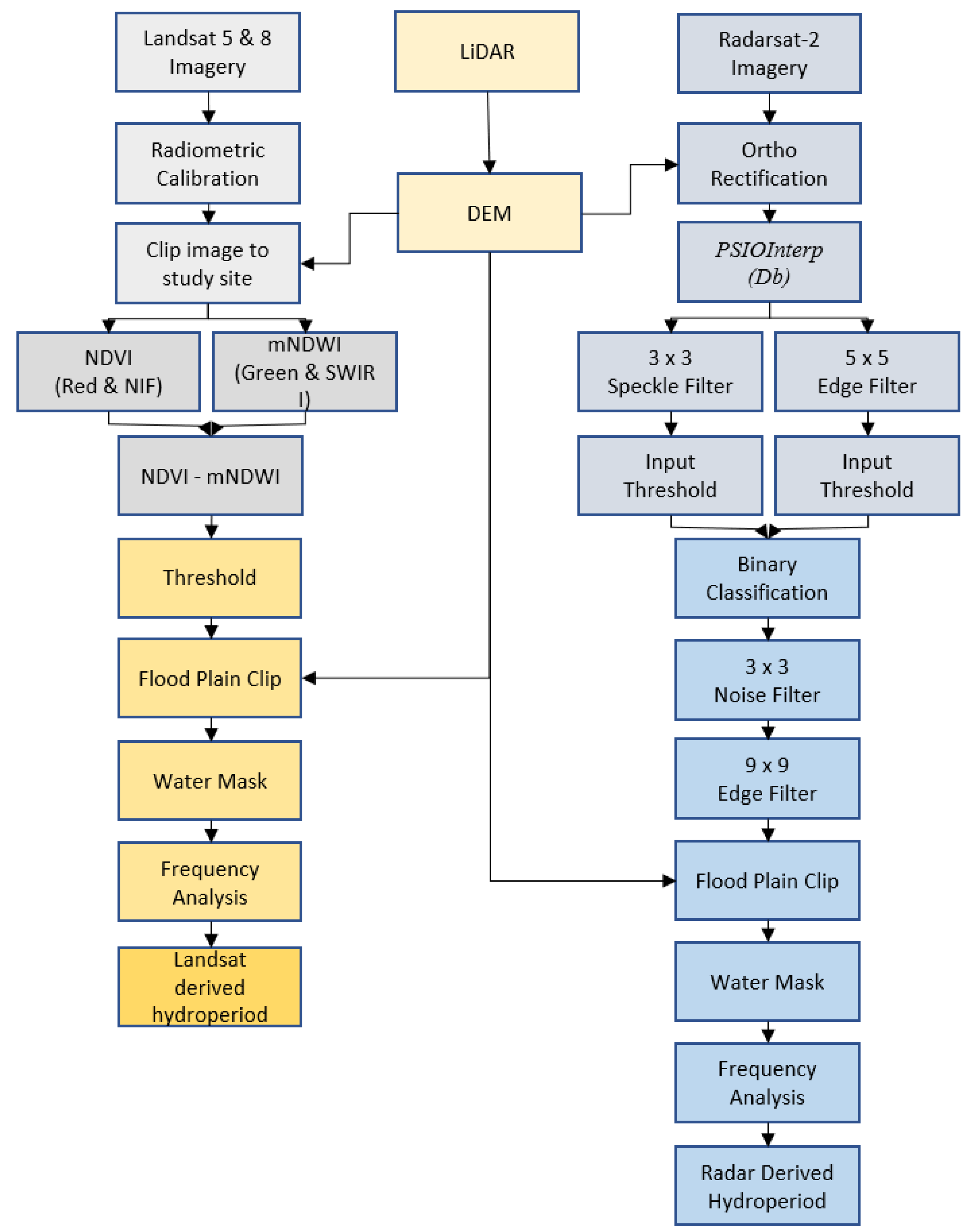
2.3. Image-Based Water Mask Extraction
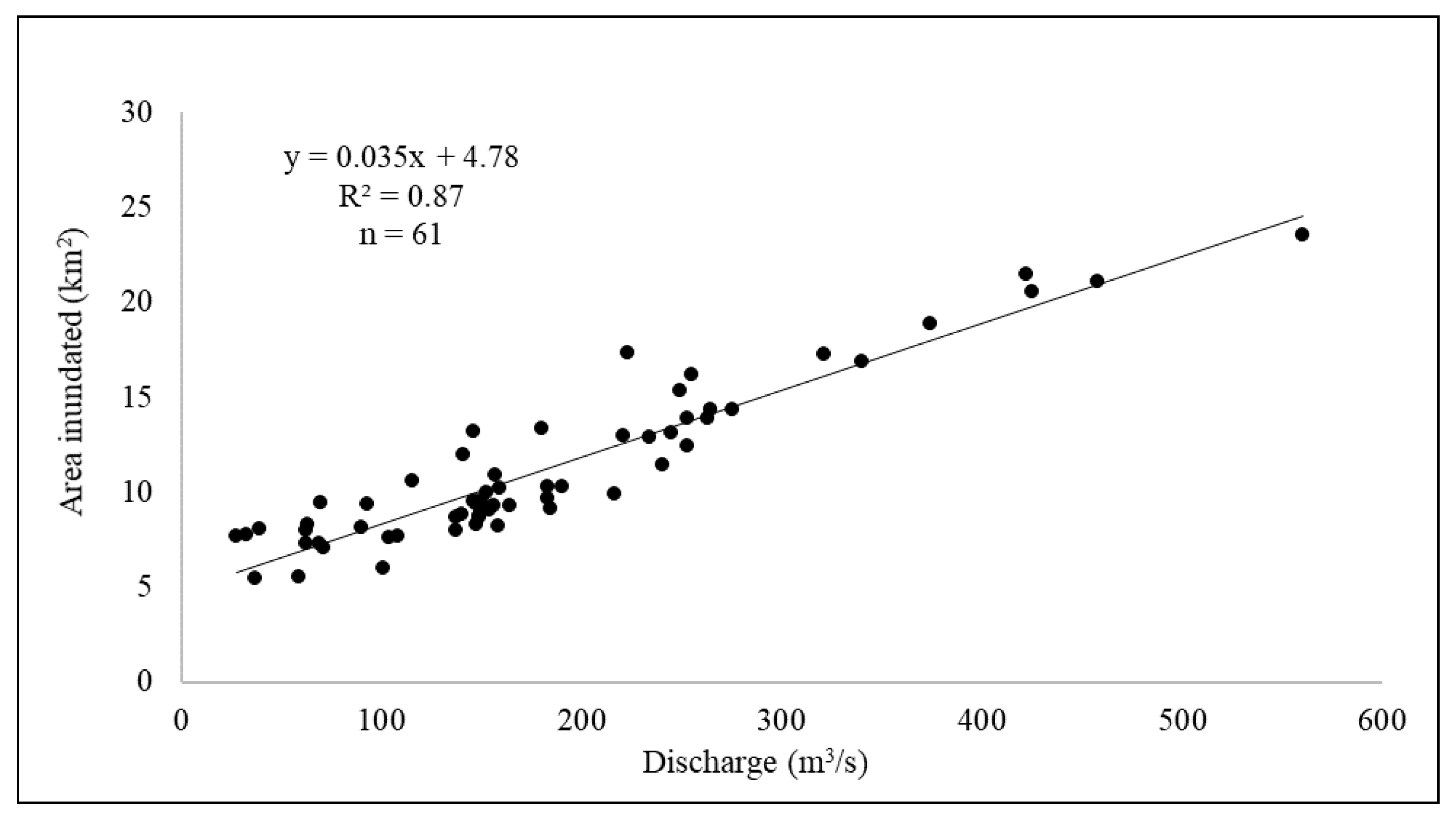
2.4. Hydroperiod Frequency Analysis
3. Results
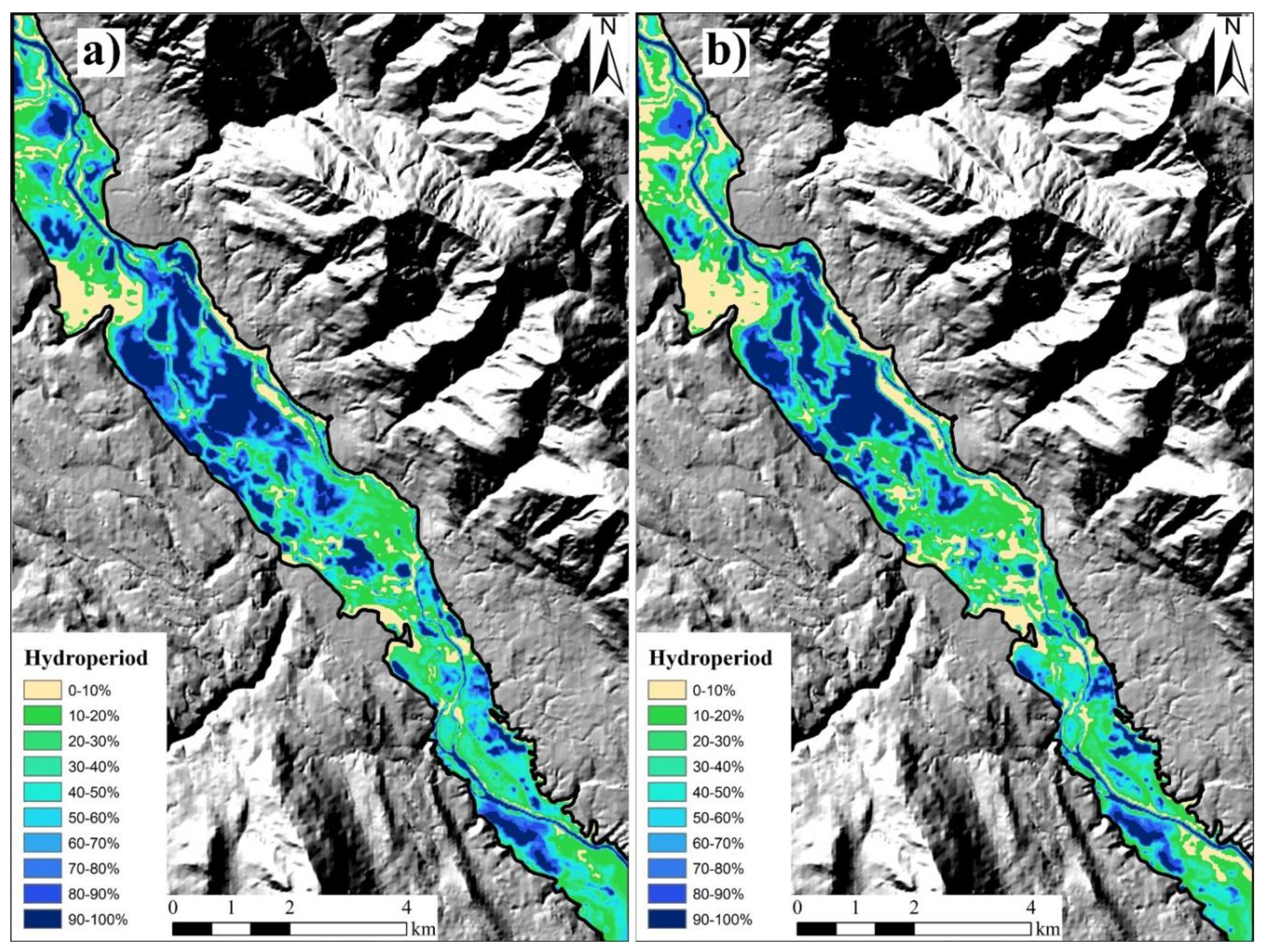
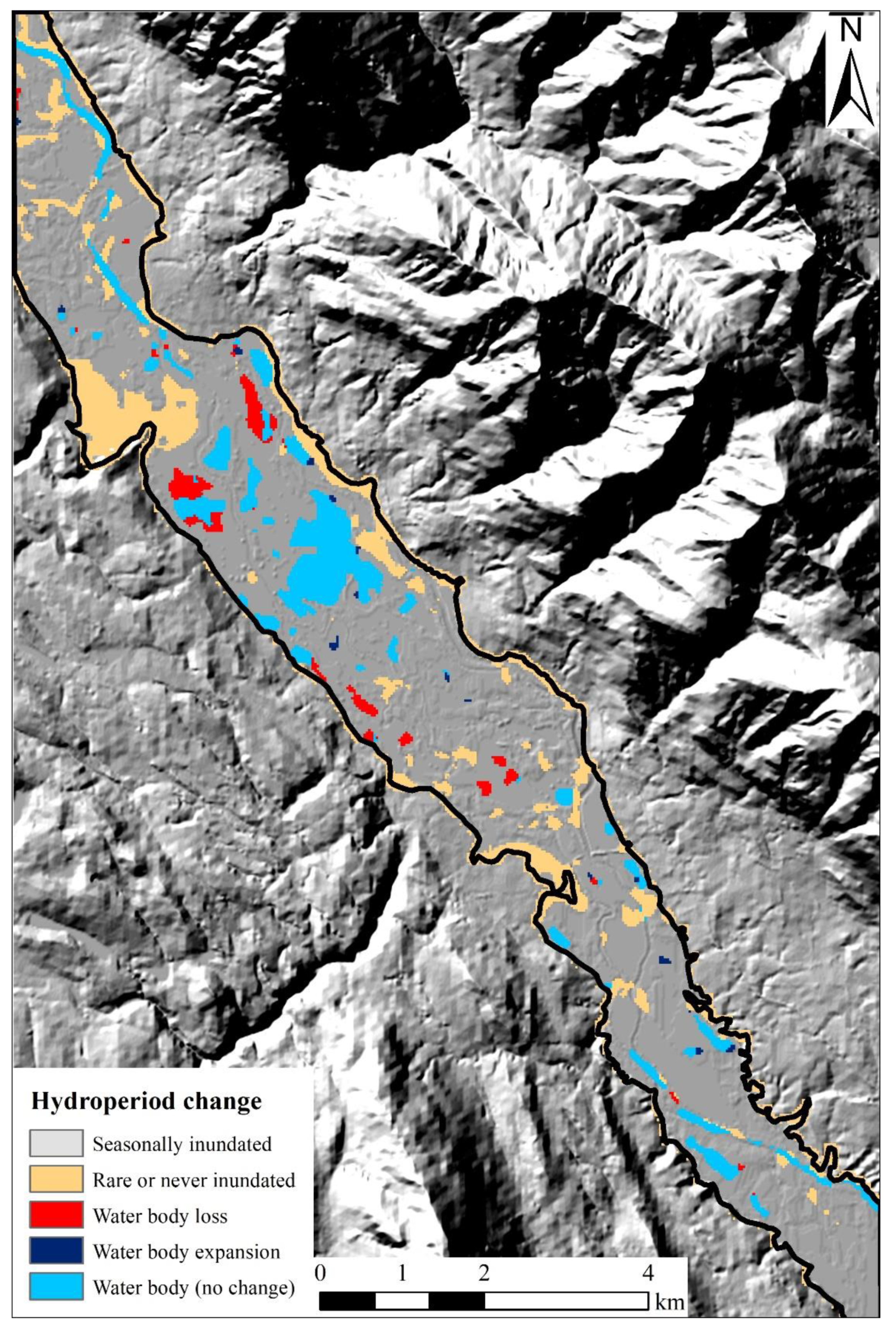
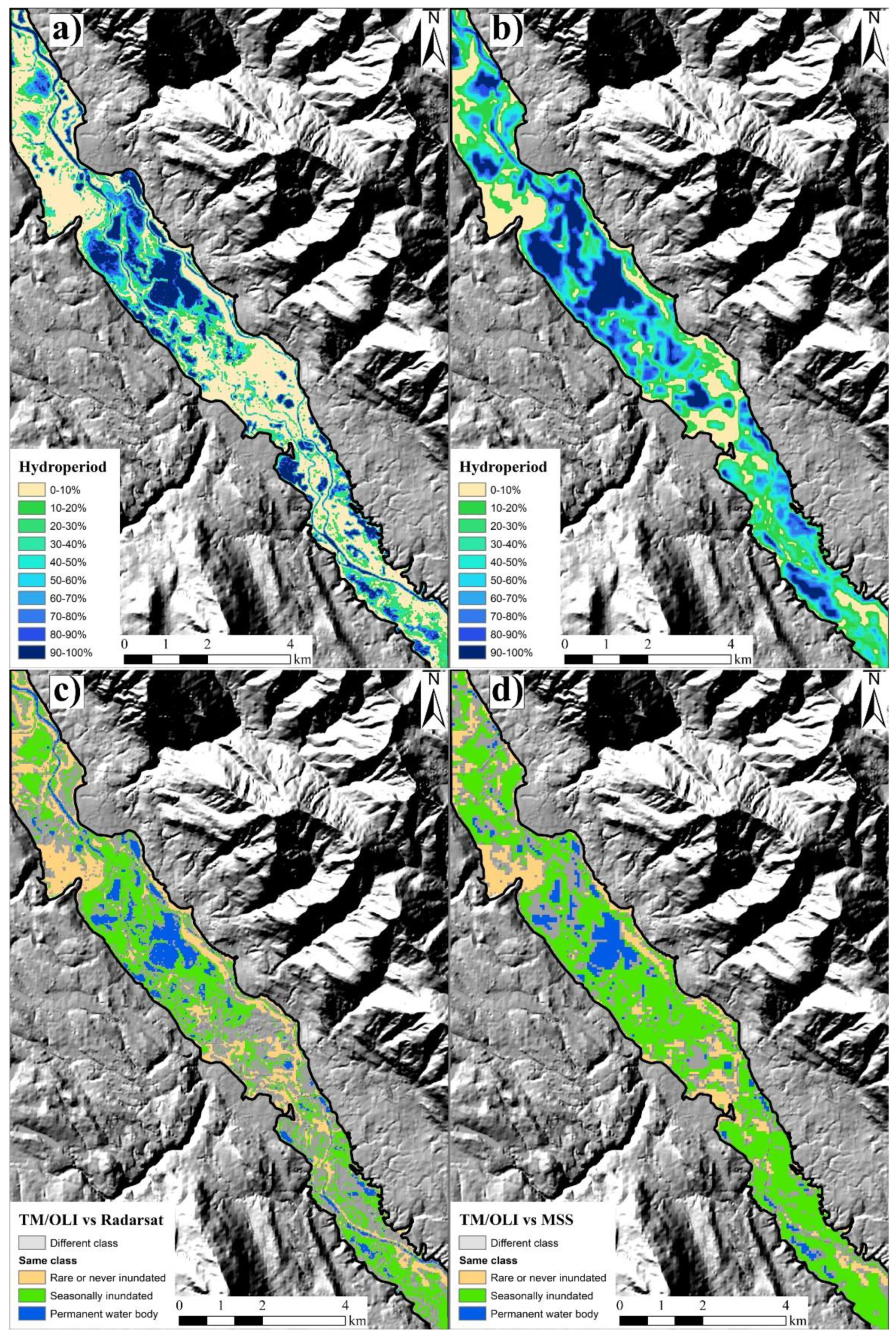
3.1. Long-Term Hydroperiod Comparison
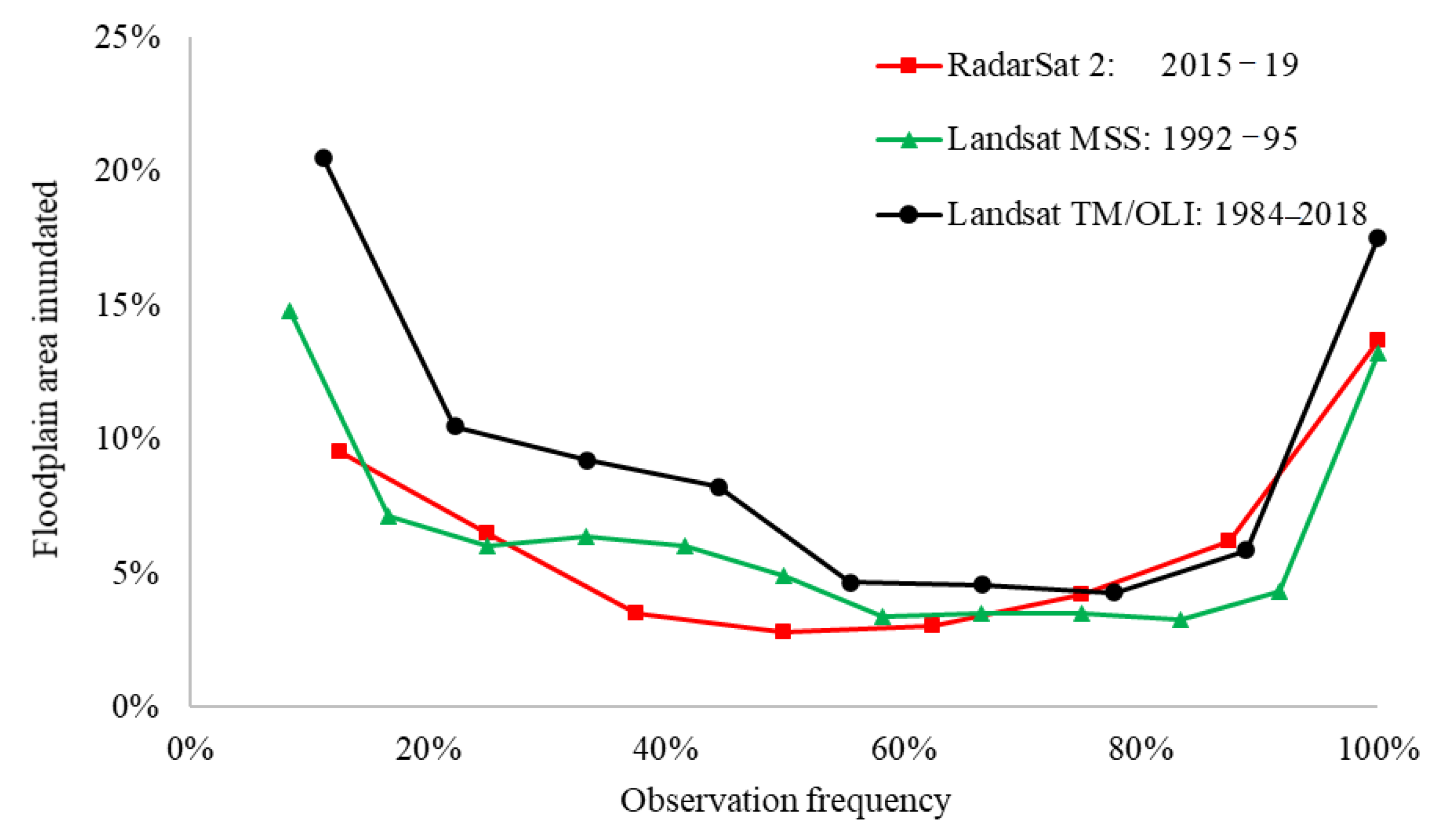
3.2. Landsat MSS and Radarsat 2 Hydroperiod
4. Discussion
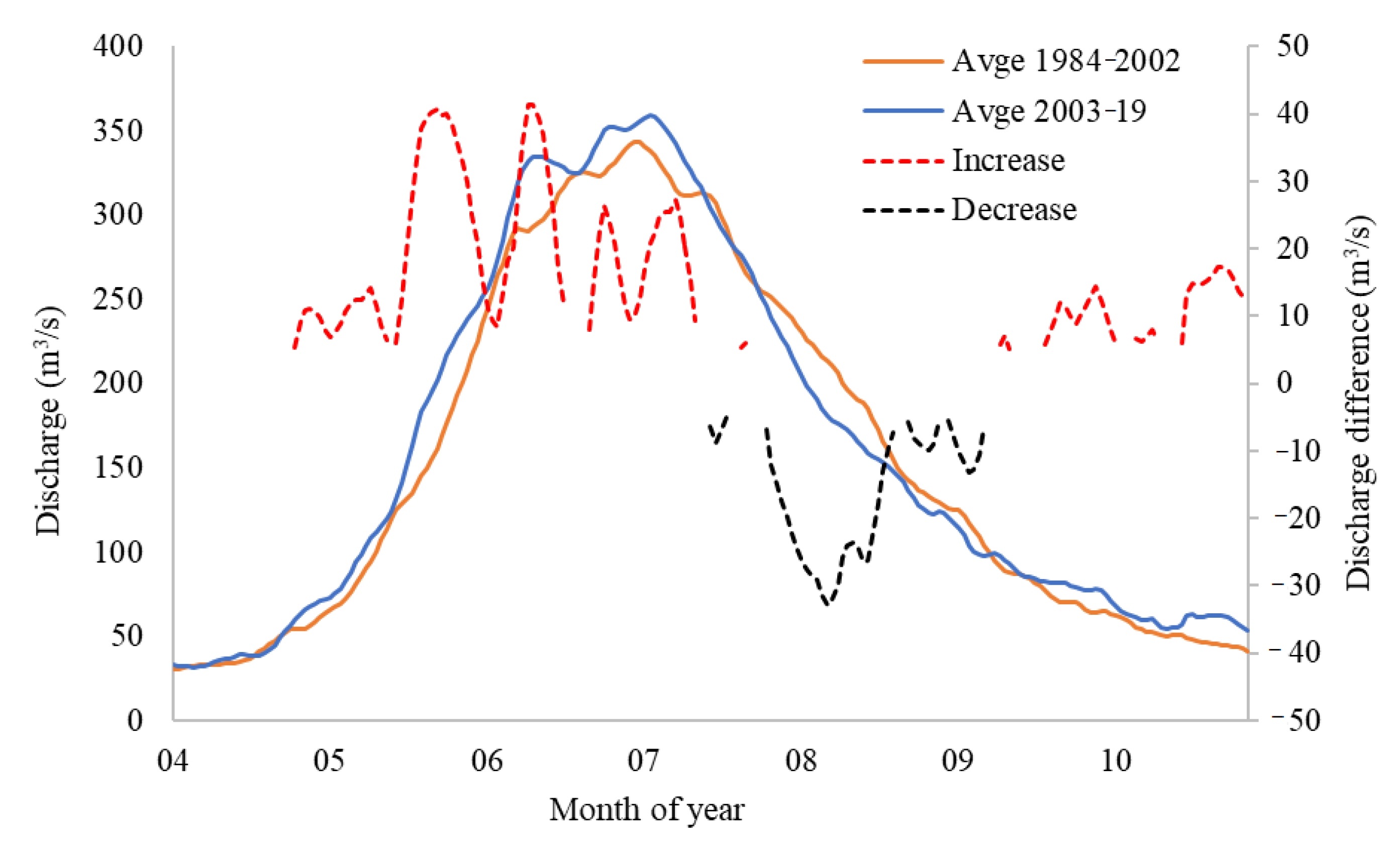
4.1. Long-Term Changes in Floodplain Wetland Hydroperiod
4.2. Extending the Hydroperiod
5. Conclusions
Author Contributions
Funding
Acknowledgments
Conflicts of Interest
References
- Blaustein, A.R.; Han, B.A.; Relyea, R.A.; Johnson, P.T.; Buck, J.C.; Gervasi, S.S.; Kats, L.B. The complexity of amphibian population declines: Understanding the role of cofactors in driving amphibian losses. Ann. N. Y. Acad. Sci. 2011, 1223, 108–119. [Google Scholar] [CrossRef] [PubMed]
- Davidson, N.C. How much wetland has the world lost? Long-term and recent trends in global wetland area. Mar. Freshw. Res. 2014, 65, 934–941. [Google Scholar] [CrossRef]
- Wisser, D.; Fekete, B.M.; Vörösmarty, C.; Schumann, A. Reconstructing 20th century global hydrography: A contribution to the Global Terrestrial Network-Hydrology (GTN-H). Hydrol. Earth Syst. Sci. 2010, 14. [Google Scholar] [CrossRef]
- Kettridge, N.; Waddington, J. Towards quantifying the negative feedback regulation of peatland evaporation to drought. Hydrol. Process. 2014, 28, 3728–3740. [Google Scholar] [CrossRef]
- Turetsky, M.R.; Kane, E.S.; Harden, J.W.; Ottmar, R.D.; Manies, K.L.; Hoy, E.; Kasischke, E.S. Recent acceleration of biomass burning and carbon losses in Alaskan forests and peatlands. Nat. Geosci. 2011, 4, 27–31. [Google Scholar] [CrossRef]
- Zhao, J.; SMalone, L.; Oberbauer, S.F.; Olivas, P.C.; Schedlbauer, J.L.; Staudhammer, C.L.; Starr, G. Intensified inundation shifts a freshwater wetland from a CO2 sink to a source. Glob. Chang. Biol. 2019, 25, 3319–3333. [Google Scholar] [CrossRef]
- Junk, W.J.; Bayley, P.B.; Sparks, R.E. The flood pulse concept in river-floodplain systems. Can. Spec. Publ. Fish. Aquat. Sci. 1989, 106, 110–127. [Google Scholar]
- Tockner, K.; Malard, F.; Ward, J. An extension of the flood pulse concept. Hydrol. Process. 2000, 14, 2861–2883. [Google Scholar] [CrossRef]
- Whited, D.C.; Lorang, M.S.; Harner, M.J.; Hauer, F.R.; Kimball, J.S.; Stanford, J.A. Climate, hydrologic disturbance, and succession: Drivers of floodplain pattern. Ecology 2007, 88, 940–953. [Google Scholar] [CrossRef]
- Lyon, S.W.; Laudon, H.; Seibert, J.; Mörth, M.; Tetzlaff, D.; Bishop, K.H. Controls on snowmelt water mean transit times in northern boreal catchments. Hydrol. Process. 2010, 24, 1672–1684. [Google Scholar] [CrossRef]
- Allen, C.; Gonzales, R.; Parrott, L. Modelling the contribution of ephemeral wetlands to landscape connectivity. Ecol. Model. 2020, 419, 108944. [Google Scholar] [CrossRef]
- Brooks, G.C.; Smith, J.A.; Gorman, T.A.; Haas, C.A. Discerning the Environmental Drivers of Annual Migrations in an Endangered Amphibian. Copeia 2019, 107, 270–276. [Google Scholar] [CrossRef]
- Gownaris, N.J.; Pikitch, E.K.; Ojwang, W.O.; Michener, R.; Kaufman, L. Predicting species’ vulnerability in a massively perturbed system: The fishes of Lake Turkana, Kenya. PLoS ONE 2015, 10, e0127027. [Google Scholar] [CrossRef] [PubMed]
- Gownaris, N.J.; Rountos, K.J.; Kaufman, L.; Kolding, J.; Lwiza, K.M.; Pikitch, E.K. Water level fluctuations and the ecosystem functioning of lakes. J. Great Lakes Res. 2018, 44, 1154–1163. [Google Scholar] [CrossRef]
- Klein, E.; Berg, E.E.; Dial, R. Wetland drying and succession across the Kenai Peninsula Lowlands, south-central Alaska. Can. J. For. Res. 2005, 35, 1931–1941. [Google Scholar] [CrossRef]
- Owen, R.K.; EWebb, B.; Haukos, D.A.; Goyne, K.W. Projected climate and land use changes drive plant community composition in agricultural wetlands. Environ. Exp. Bot. 2020, 175, 104039. [Google Scholar] [CrossRef]
- Riordan, B.; Verbyla, D.; McGuire, A.D. Shrinking ponds in subarctic Alaska based on 1950–2002 remotely sensed images. J. Geophys. Res. Biogeosci. 2006, 111. [Google Scholar] [CrossRef]
- Roulet, N.T. Peatlands, carbon storage, greenhouse gases, and the Kyoto Protocol: Prospects and significance for Canada. Wetlands 2000, 20, 605–615. [Google Scholar] [CrossRef]
- Ozesmi, S.L.; Bauer, M.E. Satellite remote sensing of wetlands. Wetl. Ecol. Manag. 2002, 10, 381–402. [Google Scholar] [CrossRef]
- Kammerer, J.C. Largest rivers in the United States. In Water Resources Investigations Open File Report 87-242, August 1987; Available from Books and Open File Report Section; USGS: Denver, CO, USA, 1987. [Google Scholar]
- Feulner, G.; Rahmstorf, S.; Levermann, A.; Volkwardt, S. On the origin of the surface air temperature difference between the hemispheres in Earth’s present-day climate. J. Clim. 2013, 26, 7136–7150. [Google Scholar] [CrossRef]
- Rokaya, P.; Peters, D.L.; Elshamy, M.; Budhathoki, S.; Lindenschmidt, K.E. Impacts of future climate on the hydrology of a northern headwaters basin and its implications for a downstream deltaic ecosystem. Hydrol. Process. 2020, 34, 1630–1646. [Google Scholar] [CrossRef]
- Leach, J.A.; Buttle, J.M.; Webster, K.L.; Hazlett, P.W.; Jeffries, D.S. Travel times for snowmelt-dominated headwater catchments: Influences of wetlands and forest harvesting, and linkages to stream water quality. Hydrol. Process. 2020, 34, 2154–2175. [Google Scholar] [CrossRef]
- Brahney, J.; Weber, F.; Foord, V.; Janmaat, J.; Curtis, P.J. Evidence for a climate-driven hydrologic regime shift in the Canadian Columbia Basin. Can. Water Resour. J. Rev. Can. Ressour. Hydr. 2017, 42, 179–192. [Google Scholar] [CrossRef]
- Moore, R.D.; Pelto, B.; Menounos, B.; Hutchinson, D. Detecting the Effects of Sustained Glacier Wastage on Streamflow in Variably Glacierized Catchments. Front. Earth Sci. 2020, 8, 136. [Google Scholar] [CrossRef]
- Bürger, G.; Schulla, J.; Werner, A. Estimates of future flow, including extremes, of the Columbia River headwaters. Water Resour. Res. 2011, 47. [Google Scholar] [CrossRef]
- Carver, M. Water Monitoring and Climate Change in the Upper Columbia Basin: Summary of Current Status and Opportunities; Columbia Basin Trust: Castlegar, BC, Canada, 2017. [Google Scholar]
- MacDonald, R.; Chernos, M. Hydrological Assessment of the Upper Columbia River Watershed; MacHydro Consultants Ltd.: Cranbrook, BC, Canada, 2020; p. 64. [Google Scholar]
- Jost, G.; Moore, R.; Menounos, B.; Wheate, R. Quantifying the contribution of glacier runoff to streamflow in the upper Columbia River Basin, Canada. Hydrol. Earth Sys. Sci. 2012, 16. [Google Scholar] [CrossRef]
- Moore, R.D.; Fleming, S.W.; Menounos, B.; Wheate, R.; Fountain, A.; Stahl, K.; Holm, K.; Jakob, M. Glacier change in western North America: Influences on hydrology, geomorphic hazards and water quality. Hydrol. Process. 2009, 23, 42–61. [Google Scholar] [CrossRef]
- Stahl, K.; Moore, R.D. Influence of watershed glacier coverage on summer streamflow in British Columbia, Canada. Water Resour. Res. 2006, 42. [Google Scholar] [CrossRef]
- Schnorbus, M.; Bennett, K.; Werner, A.; Berland, A. Hydrologic impacts of climate change in the Peace, Campbell and Columbia Watersheds, British Columbia, Canada; Pacific Climate Impacts Consortium, University of Victoria: Victoria, BC, Canada, 2011; Volume 157, pp. 2005–2012. [Google Scholar]
- Barnett, T.P.; Adam, J.C.; Lettenmaier, D.P. Potential impacts of a warming climate on water availability in snow-dominated regions. Nat. Cell Biol. 2005, 438, 303–309. [Google Scholar] [CrossRef]
- Hamlet, A.F.; Elsner, M.M.; Mauger, G.S.; Lee, S.-Y.; Tohver, I.; Norheim, R.A. An Overview of the Columbia Basin Climate Change Scenarios Project: Approach, Methods, and Summary of Key Results. Atmos. Ocean 2013, 51, 392–415. [Google Scholar] [CrossRef]
- Knowles, N.; Dettinger, M.D.; Cayan, D.R. Trends in Snowfall versus Rainfall in the Western United States. J. Clim. 2006, 19, 4545–4559. [Google Scholar] [CrossRef]
- Stewart, I.T.; Cayan, D.R.; Dettinger, M. Changes toward Earlier Streamflow Timing across Western North America. J. Clim. 2005, 18, 1136–1155. [Google Scholar] [CrossRef]
- Becker, C.G.; Fonseca, C.R.; Haddad, C.F.B.; Prado, P.I. Habitat Split as a Cause of Local Population Declines of Amphibians with Aquatic Larvae. Conserv. Biol. 2009, 24, 287–294. [Google Scholar] [CrossRef]
- Hof, C.; Araújo, M.B.; Jetz, W.; Rahbek, C. Additive threats from pathogens, climate and land-use change for global amphibian diversity. Nat. Cell Biol. 2011, 480, 516–519. [Google Scholar] [CrossRef] [PubMed]
- Jakob, C.; Poizat, G.; Veith, M.; Seitz, A.; Crivelli, A.J. Breeding phenology and larval distribution of amphibians in a Mediterranean pond network with unpredictable hydrology. Hydrobiologia 2003, 499, 51–61. [Google Scholar] [CrossRef]
- Evers, D.; Paruk, J.; McIntyre, J.; Barr, J.; Billerman, S. Common Loon (Gavia immer), Version 1.0; Cornell Lab of Ornithology Ithaca: Lansing, NY, USA, 2020. [Google Scholar]
- McIntyre, J.W.; Olson, A. The Common Loon: Spirit of Northern Lakes; University of Minnesota Press: Minneapolis, MN, USA, 1988. [Google Scholar]
- Vermeer, K. Some aspects of the nesting requirements of common loons in Alberta. Wilson Bull. 1973, 85, 429–435. [Google Scholar]
- Carli, C.M.; Bayley, S.E. River connectivity and road crossing effects on floodplain vegetation of the upper Columbia River, Canada. Écoscience 2015, 22, 97–107. [Google Scholar] [CrossRef]
- Reese, G.C.; Skagen, S.K. Modeling nonbreeding distributions of shorebirds and waterfowl in response to climate change. Ecol. Evol. 2017, 7, 1497–1513. [Google Scholar] [CrossRef]
- Rooney, R.; Carli, C.; Bayley, S.E. River Connectivity Affects Submerged and Floating Aquatic Vegetation in Floodplain Wetlands. Wetlands 2013, 33, 1165–1177. [Google Scholar] [CrossRef]
- Sofaer, H.R.; Skagen, S.K.; Barsugli, J.J.; Rashford, B.S.; Reese, G.C.; Hoeting, J.A.; Wood, A.W.; Noon, B.R. Projected wetland densities under climate change: Habitat loss but little geographic shift in conservation strategy. Ecol. Appl. 2016, 26, 1677–1692. [Google Scholar] [CrossRef]
- Ashpole, S.; Bishop, C.A.; Murphy, S.D. Reconnecting Amphibian Habitat through Small Pond Construction and Enhancement, South Okanagan River Valley, British Columbia, Canada. Diversity 2018, 10, 108. [Google Scholar] [CrossRef]
- Brisco, B.; Ahern, F.; Murnaghan, K.; White, L.; Canisus, F.; Lancaster, P. Seasonal Change in Wetland Coherence as an Aid to Wetland Monitoring. Remote Sens. 2017, 9, 158. [Google Scholar] [CrossRef]
- Irwin, K.; Beaulne, D.; Braun, A.; Fotopoulos, G. Fusion of SAR, Optical Imagery and Airborne LiDAR for Surface Water Detection. Remote Sens. 2017, 9, 890. [Google Scholar] [CrossRef]
- Montgomery, J.; Brisco, B.; Chasmer, L.; DeVito, K.J.; Cobbaert, D.; Hopkinson, C. SAR and Lidar Temporal Data Fusion Approaches to Boreal Wetland Ecosystem Monitoring. Remote Sens. 2019, 11, 161. [Google Scholar] [CrossRef]
- Montgomery, J.S.; Hopkinson, C.; Brisco, B.; Patterson, S.; Rood, S.B. Wetland hydroperiod classification in the western prairies using multitemporal synthetic aperture radar. Hydrol. Process. 2018, 32, 1476–1490. [Google Scholar] [CrossRef]
- Tetteh, G.O.; Schönert, M. Automatic Generation of Water Masks from RapidEye Images. J. Geosci. Environ. Prot. 2015, 3, 17–23. [Google Scholar] [CrossRef]
- Vinayaraj, P.; Oishi, Y.; Nakamura, R. Development of an Automatic Dynamic Global Water Mask Using Landsat-8 Images. In Proceedings of the IGARSS 2018—2018 IEEE International Geoscience and Remote Sensing Symposium, Institute of Electrical and Electronics Engineers (IEEE). Valencia, Spain, 22–27 July 2018; pp. 822–825. [Google Scholar]
- Fang-Fang, Z.; Bing, Z.; Jun-Sheng, L.; Qian, S.; Yuanfeng, W.; Yang, S. Comparative Analysis of Automatic Water Identification Method Based on Multispectral Remote Sensing. Procedia Environ. Sci. 2011, 11, 1482–1487. [Google Scholar] [CrossRef]
- Zhou, W.; Li, Z.; Ji, S.; Hua, C.; Fan, W. A new index model NDVI-MNDWI for water object extraction in hybrid area. In Proceedings of the International Conference on Geo-Informatics in Resource Management and Sustainable Ecosystem, Ypsilanti, MI, USA, 3–5 October 2014; Springer: Berlin/Hedelberg, Germany, 2014. [Google Scholar]
- Siles, G.; Trudel, M.; Peters, D.L.; Leconte, R. Hydrological monitoring of high-latitude shallow water bodies from high-resolution space-borne D-InSAR. Remote Sens. Environ. 2020, 236, 111444. [Google Scholar] [CrossRef]
- Schmitt, A.; Leichtle, T.; Huber, M.; Roth, A. On the use of dual-co-polarized TerraSAR-X data for wetland monitoring. Int. Arch. Photogramm. Remote Sens. Spat. Inf. Sci. 2012, 39, B7. [Google Scholar] [CrossRef]
- Chen, Z.; White, L.; Banks, S.; Behnamian, A.; Montpetit, B.; Pasher, J.; Duffe, J.; Bernard, D. Characterizing marsh wetlands in the Great Lakes Basin with C-band InSAR observations. Remote Sens. Environ. 2020, 242, 111750. [Google Scholar] [CrossRef]
- Brisco, B. Mapping and Monitoring Surface Water and Wetlands with Synthetic Aperture Radar. Remote Sens. Wetl. 2015, 119–136. [Google Scholar] [CrossRef]
- Di Baldassarre, G.; Schumanni, D.G.; Brandimarte, L.; Bates, P.B. Timely Low Resolution SAR Imagery To Support Floodplain Modelling: A Case Study Review. Surv. Geophys. 2011, 32, 255–269. [Google Scholar] [CrossRef]
- Bolanos, S.; Stiff, D.; Brisco, B.; Pietroniro, A. Operational Surface Water Detection and Monitoring Using Radarsat 2. Remote Sens. 2016, 8, 285. [Google Scholar] [CrossRef]
- Mahoney, C.; Merchant, M.A.; Boychuk, L.; Hopkinson, C.; Brisco, B. Automated SAR Image Thresholds for Water Mask Production in Alberta’s Boreal Region. Remote Sens. 2020, 12, 2223. [Google Scholar] [CrossRef]
- Martinis, S.; Kuenzer, C.; Wendleder, A.; Huth, J.; Twele, A.; Roth, A.; Dech, S. Comparing four operational SAR-based water and flood detection approaches. Int. J. Remote Sens. 2015, 36, 3519–3543. [Google Scholar] [CrossRef]
- Crasto, N.; Hopkinson, C.; Forbes, D.; Lesack, L.; Marsh, P.; Spooner, I.; van der Sanden, J. A LiDAR-based decision-tree classification of open water surfaces in an Arctic delta. Remote Sens. Environ. 2015, 164, 90–102. [Google Scholar] [CrossRef]
- Chasmer, L.; Hopkinson, C.; Veness, T.; Quinton, W.; Baltzer, J. A decision-tree classification for low-lying complex land cover types within the zone of discontinuous permafrost. Remote Sens. Environ. 2014, 143, 73–84. [Google Scholar] [CrossRef]
- Goodale, R.; Hopkinson, C.; Colville, D.; Amirault-Langlais, D. Mapping piping plover (Charadrius melodus melodus) habitat in coastal areas using airborne lidar data. Can. J. Remote Sens. 2007, 33, 519–533. [Google Scholar] [CrossRef]
- Ameli, A.A.; Creed, I.F. Quantifying hydrologic connectivity of wetlands to surface water systems. Hydrol. Earth Syst. Sci. 2017, 21, 1791–1808. [Google Scholar] [CrossRef]
- Millard, K.; Richardson, M. Wetland mapping with LiDAR derivatives, SAR polarimetric decompositions, and LiDAR–SAR fusion using a random forest classifier. Can. J. Remote Sens. 2013, 39, 290–307. [Google Scholar] [CrossRef]
- Olthof, I.; Rainville, T. Evaluating Simulated RADARSAT Constellation Mission (RCM) Compact Polarimetry for Open-Water and Flooded-Vegetation Wetland Mapping. Remote Sens. 2020, 12, 1476. [Google Scholar] [CrossRef]
- Jacques, J.-M.S.; Lapp, S.L.; Zhao, Y.; Barrow, E.; Sauchyn, D.J. Twenty-first century central Rocky Mountain river discharge scenarios under greenhouse forcing. Quat. Int. 2013, 310, 34–46. [Google Scholar] [CrossRef]
- Brisco, B.; Ahern, F.; Hong, S.-H.; Wdowinski, S.; Murnaghan, K.; White, L.; Atwood, D.K. Polarimetric Decompositions of Temperate Wetlands at C-Band. IEEE J. Sel. Top. Appl. Earth Obs. Remote Sens. 2015, 8, 3585–3594. [Google Scholar] [CrossRef]
- Chasmer, L.; Mahoney, C.; Millard, K.; Nelson, K.; Peters, D.L.; Merchant, M.A.; Hopkinson, C.; Brisco, B.; Niemann, K.O.; Montgomery, J.; et al. Remote Sensing of Boreal Wetlands 2: Methods for Evaluating Boreal Wetland Ecosystem State and Drivers of Change. Remote Sens. 2020, 12, 1321. [Google Scholar] [CrossRef]


| Record Length (years) | Number Images | Permanent Water (km2) | Max Open Water (km2) | No Open Water (km2) | |
|---|---|---|---|---|---|
| T1: 1984–2002 | 18 | 30 | 3.78 (13.2%) | 21.46 (74.9%) | 4.36 (15.2%) |
| T2: 2003–2019 | 16 | 31 | 3.18 (11.1%) | 20.50 (71.5%) | 6.59 (23.0%) |
| 1984–2019 | 35 | 61 | 2.78 (9.7%) | 23.55 (82.2%) | 4.21 (14.7%) |
| Change Direction | Floodplain Class | Area Change |
|---|---|---|
| No change | Seasonally inundated | 61.8% |
| Permanent water body | 9.7% | |
| Rare or never inundated | 14.7% | |
| Increase | Permanent water body | 1.4% |
| Rare or never inundated | 8.4% | |
| Decrease | Permanent water body | 3.5% |
| Rare or never inundated | 0.5% |
| Record Length (Years) | Number Images | Permanent Water (km2) | Max Open Water (km2) | No Open Water (km2) | |
|---|---|---|---|---|---|
| MSS: 1992–1995 | 4 | 12 | 4.07 (14.2%) | 14.94 (52.2%) | 7.28 (25.4%) |
| SAR (RS2): 2015–2019 | 5 | 8 | 3.93 (13.7%) | 7.53 (26.3%) | 14.50 (50.6%) |
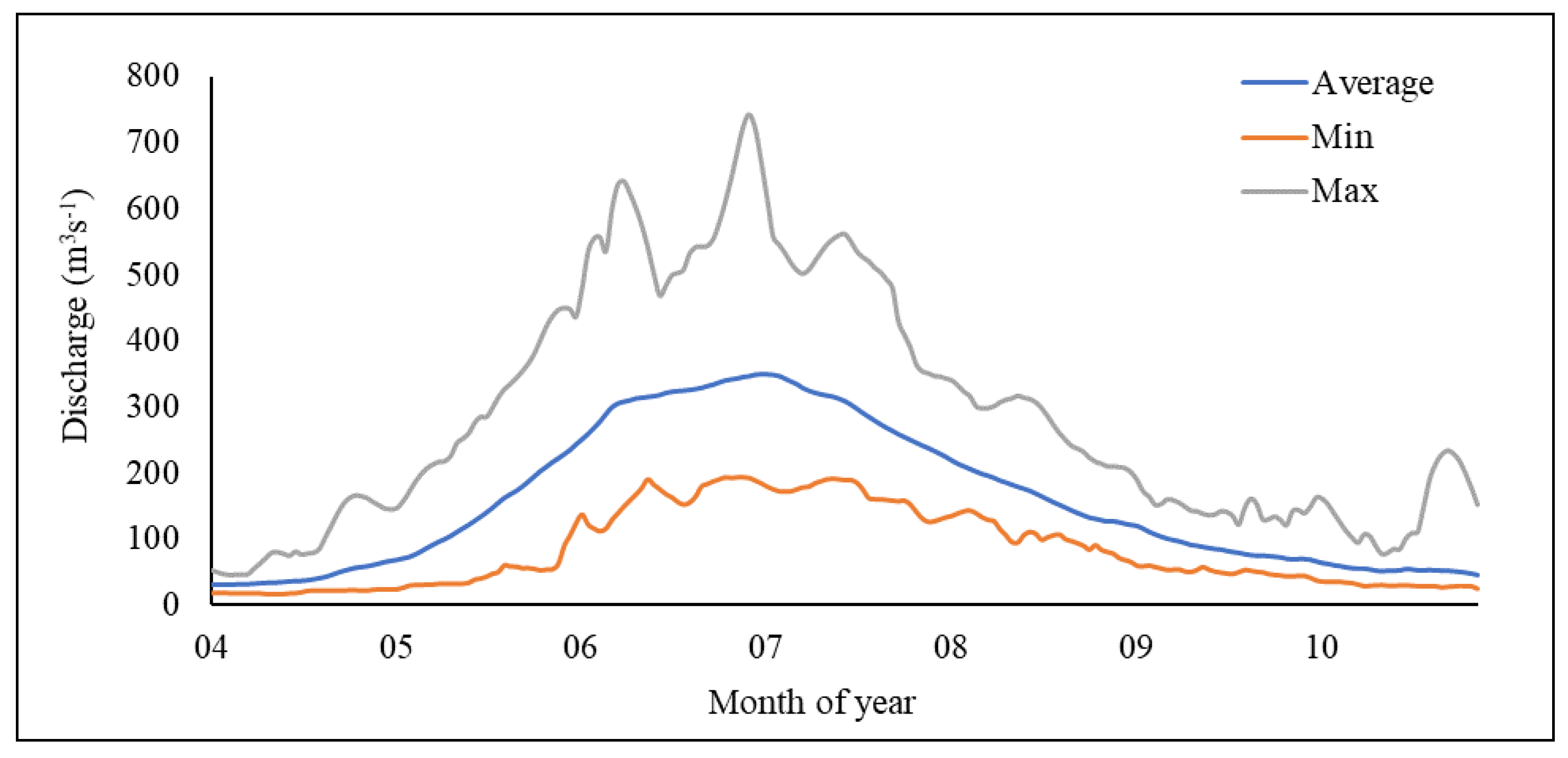
| Daily Temperature (°C) | Precipitation (mm) | Daily Discharge (m3s−1) | ||||||
|---|---|---|---|---|---|---|---|---|
| Mean Min | Mean Max | Daily Mean | Annual Mean | Max | Mean | * P25 | * P75 | |
| 1984–2002 | 0.12 | 11.85 | 6.00 | 395 | 743.0 | 156.1 | 56.4 | 237.0 |
| 2003–2019 | 0.16 | 12.25 | 6.22 | 374 | 642.0 | 162.0 | 62.4 | 235.0 |
| Difference | +0.04 | +0.40 | +0.23 | −21 | −101.0 | +5.9 | +6.0 | −2.0 |
Publisher’s Note: MDPI stays neutral with regard to jurisdictional claims in published maps and institutional affiliations.s |
© 2020 by the authors. Licensee MDPI, Basel, Switzerland. This article is an open access article distributed under the terms and conditions of the Creative Commons Attribution (CC BY) license (http://creativecommons.org/licenses/by/4.0/).
Share and Cite
Hopkinson, C.; Fuoco, B.; Grant, T.; Bayley, S.E.; Brisco, B.; MacDonald, R. Wetland Hydroperiod Change Along the Upper Columbia River Floodplain, Canada, 1984 to 2019. Remote Sens. 2020, 12, 4084. https://doi.org/10.3390/rs12244084
Hopkinson C, Fuoco B, Grant T, Bayley SE, Brisco B, MacDonald R. Wetland Hydroperiod Change Along the Upper Columbia River Floodplain, Canada, 1984 to 2019. Remote Sensing. 2020; 12(24):4084. https://doi.org/10.3390/rs12244084
Chicago/Turabian StyleHopkinson, Chris, Brendon Fuoco, Travis Grant, Suzanne E. Bayley, Brian Brisco, and Ryan MacDonald. 2020. "Wetland Hydroperiod Change Along the Upper Columbia River Floodplain, Canada, 1984 to 2019" Remote Sensing 12, no. 24: 4084. https://doi.org/10.3390/rs12244084
APA StyleHopkinson, C., Fuoco, B., Grant, T., Bayley, S. E., Brisco, B., & MacDonald, R. (2020). Wetland Hydroperiod Change Along the Upper Columbia River Floodplain, Canada, 1984 to 2019. Remote Sensing, 12(24), 4084. https://doi.org/10.3390/rs12244084