Validation of Copernicus Sea Level Altimetry Products in the Baltic Sea and Estonian Lakes

Abstract

Multi-mission satellite altimetry (e.g., ERS, Envisat, TOPEX/Poseidon, Jason) data have enabled a synoptic-scale view of ocean variations in past decades. Since 2016, the Sentinel-3 mission has provided better spatial and temporal sampling compared to its predecessors. The Sentinel-3 Ku/C Radar Altimeter (SRAL) is one of the synthetic aperture radar altimeters (SAR Altimeter) which is more precise for coastal and lake observations. The article studies the performance of the Sentinel-3 Level-2 sea level altimetry products in the coastal areas of the Baltic Sea and on two lakes of Estonia. The Sentinel-3 data were compared with (i) collocated Global Navigation Satellite System (GNSS) ship measurements, (ii) the Estonian geoid model (EST-GEOID2017) together with sea-level anomaly corrections from the tide gauges, and (iii) collocated buoy measurements. The comparisons were carried out along seven Sentinel-3A/B tracks across the Baltic Sea and Estonian lakes in 2019. In addition, the Copernicus Marine Environment Monitoring Service (CMEMS) Level-3 sea-level products and the Nucleus for European Modelling of the Ocean (NEMO) reanalysis outcomes were compared with measurements from Estonia’s 21 tide gauges and the buoy deployed offshore. Our results showed that the uncertainty of the Sentinel-3 Level-2 altimetry product was below decimetre level for the seacoast and the selected lakes of Estonia. Results from CMEMS Level-3 altimetry products showed a correlation of 0.83 (RMSE 0.18 m) and 0.91 (RMSE 0.27 m) when compared against the tide gauge measurements and the NEMO model, respectively. The overall performance of the altimetry products was very good, except in the immediate vicinity of the coastline and for the lakes, where the accuracy was nearly three times lower than for the open sea, but still acceptably good.

1. Introduction

Water level monitoring stations or tide gauges (TG) have been widely used to observe sea-level variations on the coast and their time series are considered longer and more reliable than remote sensing measurements. However, the tide gauge records might also include several other signals, such as glacial isostatic adjustment (GIA), neotectonic movements and local land subsidence since their measurements are related to the ground they are connected to. Tide gauge networks are usually sparsely distributed along the shoreline and do not all cover the same time period. Aforenamed problems are the key limitations for their use. To avoid these influences and to transform sea surface heights (SSH) into a common height system, it is recommended to use the tide gauges connected to the Global Navigation Satellite System (GNSS) stations or satellite altimetry (SA) to calculate the absolute SSH above a reference ellipsoid [1,2]. Radar altimeter is a precise ranging tool designed for measuring SSH over the open ocean at an uncertainty level of around 0.035–0.050 m [1,3,4]. Satellite altimetry has been used in sea-level variation studies for more than 30 years. The first satellite providing altimetry data was the experimental Seasat mission in the late 1970s. Satellite altimetry gained popularity in the 1990s when TOPEX/Poseidon and ERS-1 missions were launched. Nowadays, it is an important tool for understanding the topography of mesoscale eddies and the multidecadal trend of eustatic (global) sea-level rise.

Sentinel altimetry has been successfully used in the open ocean for water level monitoring, determination of wave height, storm surge, tides, etc. However, it has increasingly used to estimate mean sea-level (MSL) trends in the coastal areas where satellite data complement in situ TG time series and hydrodynamic models. Major progress was made over the last 15 years thanks to several innovative retracking algorithms in the coastal zone. Success has been furthered by the development of the Synthetic Aperture Radar Altimeter (SAR Altimeter), which performs coherent processing of groups of transmitted pulses and exploits the Delay Doppler signal of the full bandwidth [5]. The progress of altimetry data processing methods has also been driven by the improvement of geophysical corrections, such as wet/dry troposphere corrections, ionospheric delay, tidal models, and the necessary waveform retracking algorithms [6]. Additionally, several new-generation radar altimeters were launched in recent decades. For example, CryoSat-2 was launched in 2010 [7] and the two satellites of the Sentinel-3A/B (S3A/B) constellation were launched in 2016 and 2018, respectively. This new altimetry fleet provides much higher spatial resolution and lower noise, aiming at reducing land contamination in coastal radar echoes. CryoSat-2 and Sentinel-3 operating in SAR mode have a waveform footprint of 5 km², much smaller than that covered by pulse-limited altimeters in 20–30 km², such as SARAL/AltiKa and the Jason series. The along-track resolution of SAR altimeters has been increased to approximately 300 m along the flight path [8].

However, the accuracy of coastal altimetry is still affected by coexistence of the targeted water and the neighbouring terrain within a footprint [9]. Using SAR altimeters, SSH can be estimated to decimetre-level accuracy in the Baltic Sea [10] and to a couple of decimetres for small lakes with diameter less than 10 km [11]. Various validation methods are able to determine the accuracy of altimetric heights. For instance, Etcheverry et al. [12] used 478 global tide gauges to verify gridded altimetry sea-level anomaly (SLA) [12], while Ardalan et al. [13] deployed Global Positioning System (GPS) buoys to evaluate SARAL/AltiKa products. Moreover, Birgiel et al. [10] used the precise national geoid model to examine Sentinel-3 coastal product with a SAMOSA 2 retracker, and Bonnefond et al. [14] used a GPS-catamaran for validation. All these methods can be cross-validated as well.

Sentinel-3 products are categorized in three levels. Level-0 (raw) product is an internal product and is not available to users. Level-1 (SR_1_SRA) is the Level-0 product corrected for instrumental effects. Level-2 (water SR_2_WAT and land SR_2_LN) is the Level-1 product corrected for geophysical effects. Level-3 and Level-4 products are validated and are the most popular products for oceanographers. Level-3 and Level-4 include along-track and gridded data, respectively.

The main objective of this study was to validate Sentinel-3A and Sentinel-3B Level-2 altimetry products along the Estonian coast of the Baltic Sea and in two small lakes: Võrtsjärv and Lake Peipus. The second aim was to evaluate the accuracy of Level-3 altimetry products as well as the Nucleus for European Modelling of the Ocean (NEMO) reanalysis model results, which are available through the Copernicus Marine Environment Monitoring Service (CMEMS) service.

2. Material and Methods

2.1. Validation Scheme

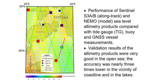
In this study, five validation strategies (Figure 1), including four field campaigns conducted in 2019, were investigated. For the Sentinel-3 Level-2 products validation, instantaneous sea surface height by altimetry (SSH_SA) was compared to instantaneous SSH from GNSS vessel campaigns (SSH_GNSS), buoy (SSH_buoy) and tide gauge measurements (SSH_TG) which were converted to the same reference system with satellite data by using a geoid model. Ideally, SSH_SA ≈ SSH_GNSS ≈ SSH_buoy ≈ SSH_TG; however, the accuracy of the geoid model, tide gauge data, GNSS-data and other factors cause uncertainties (

Table 1. Error budget of estimated uncertainties (m) of instruments and models used.

Instrument/ Model	Estimated Uncertainty	Error Source
GNSS on the vessel	±0.02	Method of measurements Method of data processing Type of antenna and receiver Antenna connection to the water
Pressure sensor-based tide gauge	±0.01–0.02	Time-dependent drift Accuracy of the sensor Connection to the height reference Stability of the height reference (vertical land motion)
Pressure sensor-based buoy	±0.01–0.02	Time-dependent drift Accuracy of the sensor Connection to the height reference
EST-GEOID2017	±0.005–0.03	Accuracy and density of the gravity data Accuracy and density of the GNSS/levelling fitting points Calculation method and accuracy of the modelling

). Note that the pressure sensor-based tide gauges are affected by a small time-dependent drift. This drift needs to be corrected by employing control readings from the staff gauge. Therefore, the uncertainty of automatic tide gauges remains on 0.01–0.02 m level [15]. The accuracy of the GNSS-derived height depends on several factors, such as the antenna and receiver, the method of measurement and processing. However, the accuracy of GNSS height based on the kinematic measurement method on the vessel should remain within a ±0.02 m level as well [16].

For validation of the Level-3 products, sea-level anomaly of the CMEMS Level-3 product (SLA_L3) and the NEMO reanalysis model output (SLA_NEMO) were compared with (i) tide gauges-based sea-level anomaly (SLA_TG) in the Gulf of Finland and the Gulf of Riga, and (ii) buoy-based sea-level anomaly (SLA_buoy) in the Gulf of Riga (Figure 1). More details on the data will be introduced in Section 2.5 and Section 2.6.

2.2. Study Sites

The Baltic Sea is a semi-enclosed water body dotted with thousands of islands and islets. Our study area is in the eastern part of the Baltic Sea (Figure 2), including the Gulf of Finland and the Gulf of Riga. The topography of the southern coast of the Gulf of Finland varies. There is a 55 metre high cliff in eastern Kunda (see the tide gauge number 2 in Figure 2) and a flat seashore along the entire western coast. Steep terrain near the coast can cause peaky waveforms and hinder the performance of retracking algorithms. The Gulf of Riga has a gently sloping and sandy seashore. However, there are many islands in the northern part of the Gulf which can make the altimetry measurements challenging along the fragmental pass-overs.

Lake Peipus (Lake Peipsi) and Lake Võrtsjärv are the two largest lakes in Estonia (Figure 2), with a surface area of 3555 km² and 270 km², respectively. Lake Peipus is the fifth largest lake in Europe, with an average depth of 7.1 m and a max depth of 15.3 m. Võrtsjärv is very shallow with an average depth of 2.7 m and a maximum depth of only 6 m.

Sentinel-3 tracks for the GNSS vessel campaigns and buoy location were selected in such a way that in situ measurements could be matched with nearly simultaneous satellite observations in the selected waterbodies (Gulf of Finland, Gulf of Riga, Lake Peipus and Võrtsjärv). This is shown in Figure 2. Additionally, three tracks for the geoid-based sea surface height validation were chosen. Thus, the following satellite data were used in our analysis: data from S3A pass 186, S3A pass 397 and S3B pass 397 (Gulf of Riga); data from S3B pass 625, S3A pass 186 (Gulf of Finland); data from S3B pass 321 (Lake Peipus); and data from S3B pass 528 (Lake Võrtsjärv).

2.3. Geoid Model EST-GEOID2017

Since sea-level variations of tidal origin are less than 0.10 m in the study area of the Baltic Sea [17], precise geoid model is one of the best reference surfaces for validating altimetric heights. The Estonian geoid model (EST-GEOID2017) is a quasi-geoid model covering 57° N–60° N and 20° E–30° E, with a spatial resolution of 1′ × 2′ which gives geoid undulation (N) above the World Geodetic System 1984 (WGS84) reference ellipsoid. Its long-wavelength information refers to the GOCO05s global gravity model [18]. Additionally, nearly 50,000 gravity points were used with an average formal uncertainty of 0.75 mGal, whereas within the Estonian mainland and islands, the uncertainty of gravity data is mostly within 0.5 mGal (see [19] for more details). The EST-GEOID2017 model is very smooth on the mainland (Figure 2) and its GNSS-levelling-based accuracy remains within ±0.005 m [19]. This means that the accuracy of the geoid model in the coastal zones of the lakes should also be around ±0.005 m. Note that the estimated discrepancy of ±0.028 m between the model and the GNSS measurements is estimated in the Gulf of Finland [16]. Considering that the geoid model undulates over ca 5 m in Estonian territory (Figure 2), the 0.05–0.03 m overall accuracy in terms of standard deviation (STD) is superb, and the use of the EST-GEOID2017 model is therefore the main option for satellite altimetry validation in the coastal zone.

2.4. Sentinel-3 Data Products

Sentinel-3 satellites carry a dual-frequency SAR altimetry payload. The main frequency used for range measurements is the Ku-band (13.575 GHz), while the C-band (5.41 GHz) is used for ionospheric correction. The SRAL altimeter has high resolution in the along-track (300 m) and across-track (1.64 km) directions, which gives better results in the coastal areas [20] compared with the conventional pulse-limited radar altimeter. Sentinel-3 is operating in a sun-synchronous orbit with a repeat cycle of 27 days. Combining S3A and S3B, the repeat cycle between two satellites becomes 13.5 days on a regional scale and the interval between interleaved groundtracks is 27 km near the Equator, which offers a better temporal and spatial resolution and increases the chance of passing over small waterbodies.

For this study, Sentinel-3 SRAL Non Time Critical Level-2 product (SR_2_LAN) from the Estonian National Copernicus Hub (ESTHub) mirror site (https://ehdatahub.maaamet.ee/dhus/#/home) over the period from December 2018 to November 2019 were used. Note that the radar range measured between the satellite and the sea surface observed near the nadir is affected by several error sources when the signal passes through the atmosphere. Additionally, several tidal effects are involved in measuring the sea level. The corrections were provided by the data agency. The following atmospheric and geophysical corrections were used:

∑cor = Δh_iono + Δh_dry + Δh_wet + Δh_ssb + ∑h_t + h_a + h_f,

(1)

where Δh_iono is ionospheric correction; Δh_dry and Δh_wet are dry and wet tropospheric corrections, respectively; Δh_ssb is sea state bias correction; ∑h_t is sum of tide heights (solid earth, and geocentric pole tide height); h_a is inverted barometer height correction, and h_f is high frequency fluctuations of the sea surface topography correction. All these parameters are given along with each SR_2_LAN data file. More details can be found in ESA’s technical guides for Sentinel-3 SRAL/MWR Level 1 & 2 [21].

Following that, the corrected range between the satellite and the sea level was calculated:

R_cor = R + ∑cor,

(2)

where R is the directly measured distance or pseudorange between the satellite and the sea level (Figure 3). The distance is estimated with the off-centre-of-gravity (OCOG) retracking algorithm [22,23]. SSH_SA above the ellipsoid was calculated:

SSH_SA = h_SA − R_cor,

(3)

where h_SA is satellite height above WGS84 ellipsoid, which can be calculated using satellite ephemeris. SSH_SA values were calculated for all studied S3A and S3B ground tracks (Figure 2) over the period from 1 January 2019 to 1 November 2019, equivalent to 10–11 cycles for each pass.

The SAR mode of Sentinel-3 effectively reduces land-induced contamination in the radar signal by increasing the spatial resolution along the track. However, the problem still exists when the satellite azimuth direction and the coastline are not perpendicular. Therefore, Sentinel-3 measurements within 2 km of the shoreline were removed in order to reduce the influence of potentially noisy data, as demonstrated by the blue points appearing between the grey and red lines in Figure 4. Normally, the differences (ΔSSH_TG) between SSH_TG and SSH_SA remained within 0.5–1 m. However, some ΔSSH outliers could be up to 2 m or more on open water due to reflections from small islets or vessels, which is known as the ‘hooking effect’ in off-nadir measurements. In addition, coastal TG data can be influenced by coastal effects (such as storm surges, wave setup), while these effects are relatively small off the shoreline.

2.5. In Situ Data

The Estonian coastline has a dense tide gauge network, from which 23 (include two stations, Rannu-Jõesuu (22) and Mustvee (23) in the lakes) stations were selected for the study (Figure 2). Of those, 15 stations are managed by the Estonian Environmental Agency (EEA) and 8 stations are operated by the Department of Marine Systems (MSI) of Tallinn University of Technology. All these tide gauges are equipped with pressure sensors and have operated for more than ten years [15]. In 2017–2018, the automatic tide gauges as well as tide gauge rods were reconnected to the national levelling network. The automatic tide gauges record hourly sea level anomaly (SLA_TG) in the Estonian height system (EH2000). The measurements are fully compatible with the European Vertical Reference System (EVRS), because the EH2000 essentially is a national realization of the EVRS in Estonia [24].

The tide gauge data were used to estimate sea-level deviations along each altimetry track. The tide gauge data were converted to the same reference system with satellite altimetry data by using geoid undulation (N) from the Estonian geoid model EST-GEOID2017 (Equation (4)). Since the geoid model has been fitted to vertical datum, geoid surface at the tide gauge approximately coincidences with the vertical datum zero. Therefore, instantaneous SLA_TG relative to geoid was calculated from the four tide gauge records nearest to the satellite track at the time of the satellite overpass. SSH_TG above the ellipsoid WGS84 at each Sentinel-3 footprint can thus be presented as:

SSH_TG = SLA_TG + N.

(4)

For Sentinel-3 validation, the difference between SSH_SA and SSH_TG was calculated using the following equation:

ΔSSH_TG = SSH_SA − SSH_TG.

(5)

Residual difference ΔSSH_TG was further analysed. The ΔSSH_TG residuals larger than 2.5 STD were considered outliers. Residuals were plotted against distance from the coast (Figure 4). Correlation plots between SSH_SA and SSH_TG were compiled as well.

In addition, GNSS kinematic measurements on the vessels were used to validate SSH_SA over the study sites. Multiple-frequency Trimble R8s and Trimble R4-3 receivers were mounted on top of the vessel (Figure 5b). Antenna reference points were connected to the sea level (H in Figure 3) using a total station (Figure 5a). Two antennas were used to eliminate the risks when one receiver stops working and to filter out vessel fluctuations [25,26]. Measurements were carried out on the same day of the satellite overpass; the weather was calm during all measurements (

Table 2. General parameters of the GNSS kinematic measurements.

Waterbody	Gulf of Finland	Gulf of Riga	Lake Peipus	Lake Võrtsjärv
Date	25 April 2019	20 June 2019	19 June 2019	13 July 2019
Weather conditions	Light wind, waves up to 1 m	Calm, no waves	Calm, no waves	Calm, no waves
Profile length (km)	25	54	33	10
Vessel

). GNSS measurements were recorded at 2 s intervals along the altimetry ground tracks (Figure 2). The first data quality control was performed on board the vessel with the program TEQC [27]. The GNSS base stations data from the Estonian Permanent GNSS Network ESTPOS [28] and the Trimble Business Centre software were used for kinematic data processing in double difference mode. The International GNSS Service (IGS) precise ephemeris and absolute antenna calibration data were used. First, both receiver’s data were processed separately and SSH_GNSS above the ellipsoid from two receivers were compared. When the difference between the SSH_GNSS from two receivers on the same time tag was larger than ±0.10 m, the measurement was excluded from further processing. Cleaned heights from two receivers on the same time tag were averaged. Next, the temporally moving-averaged SSH_GNSS was calculated in order to smooth out the fluctuations of the vessels. The window size for the moving average filter was selected based on the velocity of the vessel and the GNSS data rate (2 s) in order to obtain window size, which is close to the altimeter along-track resolution (300 m). For example, if the vessel’s velocity was 10 m/s and the GNSS sample rate was 2 s, the moving average window 15 was chosen, since 15 × 2 × 10 = 300 m. Spatially moving-averaged SSH_GNSS above WGS84 ellipsoid were compared with SSH_SA for altimetry validation:

ΔSSH_GNSS = SSH_SA − SSH_GNSS.

(6)

Note that the error sources for the determination of ΔSSH_GNSS are: (i) errors in the determination of the GNSS antenna height from the water level; the uncertainty of the sea surface height from the GNSS antenna is at least ±0.020 m and it is possible that the GNSS antenna connection to the water level could also cause a systematic shift; and (ii) the accuracy of the GNSS solution itself (Table 1). Multiple-frequency Trimble R8s and Trimble R4-3 receivers were used for the GNSS kinematic measurements on the boat, but the vertical uncertainty could be ±0.015 m + 1 ppm RMS according to the manufacturer’s specification.

In addition, a pressure sensor-based buoy (Figure 6) was deployed on the seafloor of the Gulf of Riga (Figure 2) for five months (from June to November 2019). The crossing point of the S3A pass 186 and 397 ground tracks (58°07′12″ N and 23°32′06″ E) was chosen for the buoy location. Sea-level data were recorded by buoy at 5-min intervals. The buoy’s records referred to ellipsoid WGS84. For this, the water column height above the sensor was measured by tape and sea surface height above the ellipsoid WGS84 was measured with GNSS during the buoy mounting.

2.6. Copernicus Marine Environment Monitoring Service (CMEMS) Data Products

One of the purposes of this study was to compare the accuracy of CMEMS Level-3 (L3) along-track altimetry products (SLA_L3) [29] and NEMO reanalysis model (SLA_NEMO) [30] outcomes against SLA_TG. The along-track SLA_L3 is produced with the resolution of 7 km between measurements. The reported RMS of the differences between gridded Data Unification and Altimeter Combination System Delayed Time 2018 (DUACS DT2018) sea-level anomaly and independent along track measurements for the Baltic Sea vary approximately between 0.03 and 0.07 m [31]. The CMEMS Baltic Sea Physical Reanalysis product provides a physical reanalysis for the entire Baltic Sea area. It is produced using the ice-ocean model NEMO-Nordic [30]. The reported mean correlation between SLA_TG and SLA_NEMO for the entire Baltic Sea is 0.95 with the Root Mean Square Error (RMSE) of 0.07 m, with lower values in highly dynamic marine areas [32].

The analysed SLA data covered the time interval from 2014 to 2017 when the sea-level measurements of all methods were available. The SLA_L3 data along track was collected only from the altimeters that were operational for the specified timespan (

Table 3. Overview of the satellite altimetry missions used *.

Mission	Instrument	Ground Track Repeat Cycle (Days)	Time Interval	Measurements
SARAL	AltiKa	35	13 January 2014–31 December 2017	167
CryoSat-2	SIRAL-2	369	5 January 2014–31 December 2017	225
HY-2A	ALT	14	24 April 2014–31 December 2017	111
Jason-2	Poseidon-3	10	9 January 2014–31 December 2017	50
Jason-3	Poseidon-3B	10	30 May 2016–31 December 2017	24
Sentinel-3A	SRAL	27	1 July 2016–31 December 2017	48

* Detailed overview about the different missions’ parameters can be found from Table 1 in [33].

). The specific time interval in Table 3. is set according to the first and last collocated measurement in the dataset. The number of measurements in Table 3 is dependent on satellite orbit and location of tide gauge.

Altimetry SLA_L3 along-track data were collected at a maximum distance of 10 km from the listed gauges (mean distance 7.9 km), and the maximum time difference between SLA_TG and SLA_L3 measurements was one hour (mean time difference 18 min). For the NEMO, SLA_NEMO at the closest grid point to the station within an hour’s time difference was extracted (mean distance 1.5 km). Considering seasonal component in the MSL variations in the Baltic Sea [34,35], SLA data from all seasons were used in the comparison. Final filtering for SLA_TG, SLA_L3, and SLA_NEMO was made according to match in measurement time which resulted in the number of common, collocated measurements of 625.

A separate comparison was carried out with the data from the buoy in the Gulf of Riga (see green circle on Figure 2) to measure the accuracy of SLA_L3 along-track data as well as the reanalysis model outcomes. The SLA_L3 data was collected for time period from June to November 2019 using the same scheme, i.e., maximum distance between along track measurement and SLA_TG of 10 km and maximum time difference of one hour. The final analysis consisted of 33 unique data points (mean distance: 4.3 km; mean time difference: 16 min) in all three sources.

Data analysis results are presented as standard descriptive statistics: Pearson correlation coefficient (r), RMSE and Mean Error (ME). The statistics were calculated between SLA values since the accurate translation of modelled water levels into a common reference surface is an unresolved technical issue [34].

3. Results

3.1. Sentinel-3 Level-2 Product Validation with GNSS Campaigns

The statistics of the residuals from the Equation (6) along altimetry tracks are presented in

Table 4. Statistics of differences between the sea surface height (ΔSSH_GNSS) derived from GNSS measurements (SSH_GNSS) and sea surface height derived from altimetry (SSH_SA) according to the Equation (6).

Statistics	Gulf of Finland	Gulf of Riga	Lake Peipus	Lake Võrtsjärv
MEAN (m)	0.11	0.14	0.16	0.31
STD (m)	0.08	0.05	0.13	0.39
RMSE (m)	0.13	0.15	0.21	0.49
MIN (m)	−0.11	0.00	−0.33	−0.45
MAX (m)	0.29	0.27	0.38	0.74
Common measurements	80	180	110	30

. Note that the number of common measurements vary in different waterbodies. It is caused by the length of the GNSS transect (Table 2). According to the results in multiple locations, the two datasets in the Baltic Sea correspond better than those of inland cases; the mean (MEAN) and STD were 0.11 ± 0.08 m and 0.14 ± 0.05 m in the Gulf of Finland and the Gulf of Riga, respectively. These results also match well with the validation by the geoid model for S3B pass 625 in the Gulf of Finland on 25 April 2019 (0.11 ± 0.06 m) (Figure 7) and for S3A pass 186 in the Gulf of Riga on 20 June 2019 (0.09 ± 0.05 m) (Figure 8). In Lake Peipus and Lake Võrtsjärv, the MEAN was 0.16 ± 0.13 m and 0.31 ± 0.39 m, respectively. Again, these GNSS validation results agree with the validation results using the geoid-based water surface height, showing a discrepancy of 0.15 ± 0.14 m and 0.28 ± 0.30 m for the Lake Peipus on 19 June 2019 and for Lake Võrtsjärv on 13 July 2019, respectively (Figure 9).

3.2. Sentinel-3 Level-2 Product Validation with the Geoid-Based Sea Surface Height

We studied the waterbodies separately for validation with the geoid model. Two transects were chosen for the Gulf of Finland (Figure 2) and the residual of differences for S3A and S3B (ΔSSH_TG, Equation (5)) are presented in Figure 7. The mean ΔSSH_TG was calculated for each 25-km-long transect when the satellite passed over the gulf. The time difference between S3A and S3B overpasses is two days. It is observed that the validation results and trends for both passes (S3A pass 186 and S3B pass 625) are very similar in the Gulf of Finland, which implies a similar accuracy level for both missions. The average ΔSSH_TG for S3A and S3B was 0.02 ± 0.08 m. Note that there is no ΔSSH_TG value for S3B for May 2019 (Figure 7, cycle 25) because the ΔSSH_TG at 0.31 ± 0.55 m in this cycle is clearly an outlier. Such a big residual difference could have been caused by a local wind-driven water pile-up against the coast. After removing ΔSSH_TG from cycle 25, an average residual difference of 0.01 ± 0.06 m was obtained for the Gulf of Finland (

Table 5. Statistics of differences between the sea surface heights derived from altimetry (SSH_SA) and geoid-based sea surface height (SSH_TG) according to the Equation (5).

Statistics	Gulf of Finland	Gulf of Riga	Lake Peipus	Lake Võrtsjärv
MEAN (m)	0.01	0.00	0.14	0.13
STD (m)	0.06	0.07	0.16	0.27
RMSE (m)	0.07	0.10	0.23	0.27
MIN (m)	−0.32	−0.98	−0.56	−1.13
MAX (m)	0.33	0.58	0.98	0.78
Common measurements *	75	190 ** 445 ***	100	30

* Number of common measurements per each cycle, Figure 7, Figure 8 and Figure 9. ** Sentinel-3A pass 186. *** Sentinel-3A pass 397 and Sentinel-3B pass 397.

).

Three transects were chosen for comparison in the Gulf of Riga: S3A pass 186, S3A pass 397 and S3B pass 397 (Figure 2). The results of S3A and S3B fit quite well in the Gulf of Riga (Figure 8). S3A pass 186 showed a better fit due to the shorter transect length (54 km, from the mainland to the island). For S3A pass 397 and S3B pass 397, the transects were 133 km (from the mainland to the mainland). Larger deviations were observed in winter from December to April when stormy weather conditions prevailed. The wind set-up near the coast is proportional to tangential wind speed component squared and can reach up to ca 1 m in certain Estonian coastal locations during strong storms [35]. The average residual differences between SSH_SA and SSH_TG was 0.01 ± 0.07 m. After removing an outlier (S3A pass 397 cyc 25 (11.03.2019) ΔSSH_TG = 0.410 ± 0.600 m), the average residual difference for the Gulf of Riga is 0.00 ± 0.07 m (Table 5).

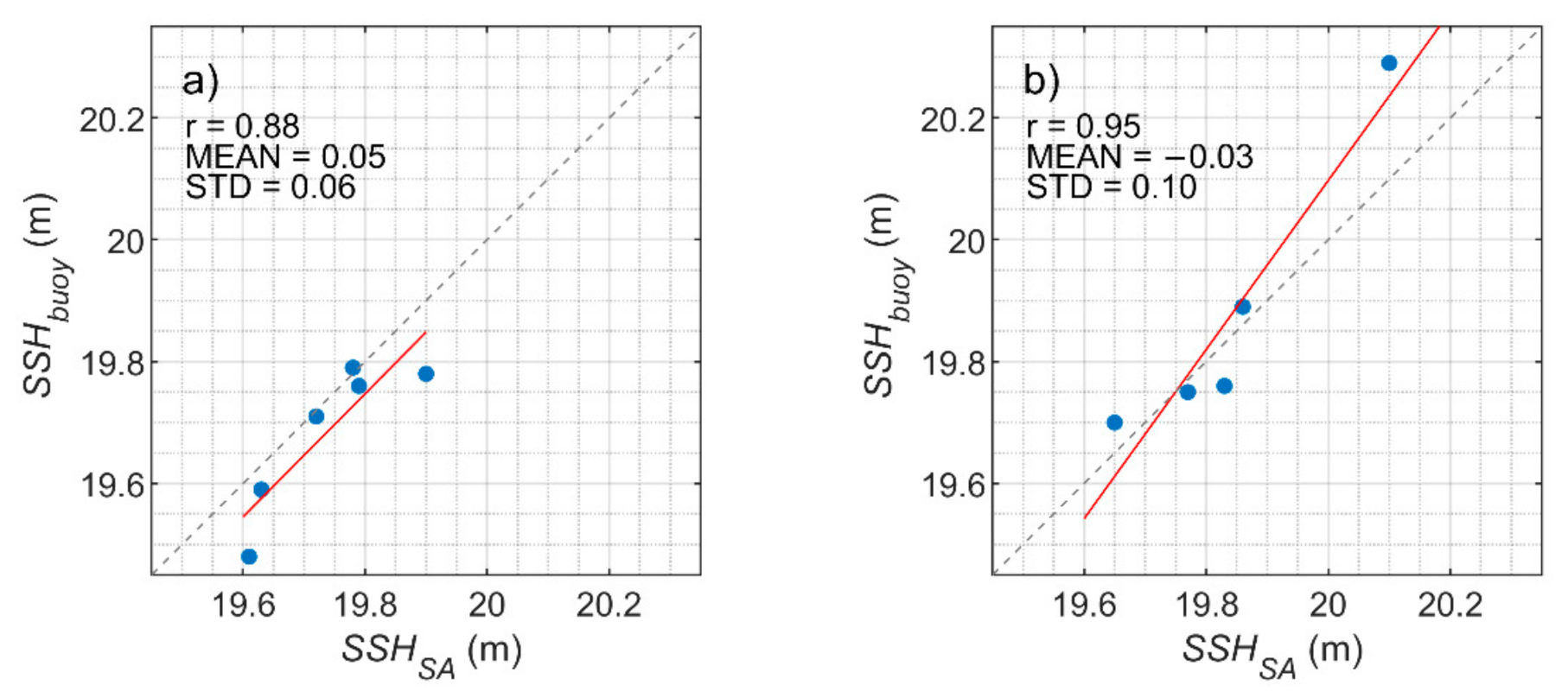
3.3. Sentinel-3 Level-2 Product Validation with Buoy Data in the Gulf of Riga

The buoy placed on the bottom of the Gulf of Riga was collecting SSH_buoy from June 2019 until November 2019. Over this period of time, satellite tracks S3A pass 186 and S3A pass 397 passed the buoy six and five times, respectively. For the validation, the mean SSH_SA for every overpass was calculated using the Level-2 altimetry product within a radius of 5 km from the buoy. It was then compared with the buoy measurements (SSH_buoy; Figure 10), representing average of twelve buoy readings taken over a time interval from half an hour before to half an hour after the satellite overpass. According to the results, the agreement between the two datasets was very good (Pearson correlation coefficients r for S3A pass 186 and S3A pass 397 were 0.88 and 0.95, respectively). The mean residual differences (ΔSSH_buoy) were 0.05 ± 0.06 m and −0.03 ± 0.10 m for S3A pass 186 and S3A pass 397, respectively.

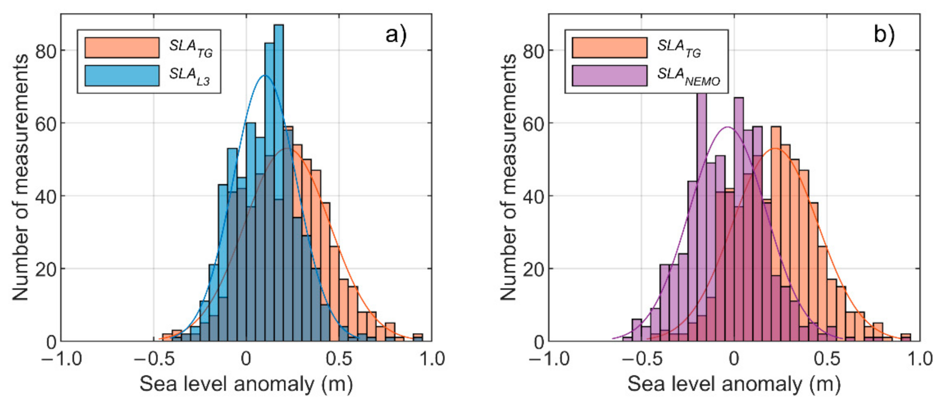
3.4. SLA_L3 and SLA_NEMO Comparison with In Situ SLA_TG Measurements

The CMEMS SLA_L3 along-track altimetry product comparison with SLA_TG measurements yielded accurate results with r = 0.83 for all stations in weighted sum (

Table 6. Overview of tide gauges (Figure 2) used for comparison with CMEMS products in the Baltic Sea. Comparison results (r and RMSE) between SLA_TG, SLA_L3 and SLA_NEMO are shown in the last four columns.

Station No	Station Name	Common Measurements	SLATG vs. SLAL3		SLATG vs. SLANEMO
			r	RMSE (m)	r	RMSE (m)
1	Dirhami	116	0.83	0.17	0.93	0.26
2	Kunda	22	0.88	0.22	0.92	0.29
3	Narva-Jõesuu	32	0.71	0.35	0.97	0.29
4	Loksa	7	0.82	0.14	0.83	0.21
5	Pirita	5	0.90	0.09	0.94	0.21
6	Paldiski	5	0.79	0.17	0.87	0.26
7	Ristna	73	0.86	0.17	0.92	0.30
8	Heltermaa	20	0.88	0.09	0.83	0.27
9	Virtsu	19	0.81	0.15	0.90	0.26
10	Roomassaare	18	0.73	0.18	0.89	0.27
11	Ruhnu	82	0.86	0.20	0.92	0.31
12	Häädemeeste	41	0.76	0.19	0.88	0.30
13	Pärnu	8	0.86	0.17	0.97	0.27
14	Muuga	15	0.80	0.17	0.83	0.27
15	Tallinna Sadam (MSI)	4	0.97	0.08	0.95	0.24
16	Paldiski (MSI)	15	0.83	0.23	0.88	0.31
17	Lehtma	82	0.85	0.14	0.93	0.21
18	Heltermaa (MSI)	21	0.85	0.10	0.87	0.24
19	Triigi	5	0.77	0.09	0.91	0.22
20	Virtsu	17	0.82	0.23	0.91	0.33
21	Rohuküla (MSI)	18	0.94	0.17	0.96	0.25
	Total/weighted average	625	0.83	0.18	0.91	0.27

, Figure 11a). The RMSE for all stations together was 0.18 m, ME = 0.12 m and the STD between SLA_TG and SLA_L3 was 0.14 m. These results were similar to previous findings for the area even though the RMSE was larger [36]. The correlation between SLA_TG and SLA_NEMO was higher (r = 0.91, Figure 11b, Table 6). However, the RMSE and ME are much higher at 0.27 m and 0.26 m, respectively, which indicated a bias in the model fields. STD between SLA_TG and SLA_NEMO was 0.10 m. The comparison with Narva-Jõesuu station (tide gauge number 3 in Figure 2, Table 6) shows the worst performance regarding its low correlation and high RMSE (0.35 m) and ME (0.30 m). A closer look at the data shows that approximately 30% of the data were collected in winter, which may be one of the reasons why the satellite results were underestimated. In addition, the exact measurement point in Narva-Jõesuu is at the mouth of Narva River which may hinder the quality of comparison results, as the dynamics of the river itself are not recorded in the satellite results within a 10 km radius.

In Figure 12, a comparison of the SLA_buoy data from the Gulf of Riga open sea station (green circle in Figure 2) with SLA_L3 data and SLA_NEMO data is shown. Surprisingly, the along-track SLA accuracy gained little to no improvement compared with the results of coastal measurements, whereas NEMO reanalysis model outcomes improved significantly in the open sea. This suggests that the NEMO reanalysis fields represent sea-level variations in the open sea with high accuracy, while in the coastal region where the sea level is influenced by various processes and factors (shallow areas, coastal effects, waves, etc.), the model reanalysis data loses some of its accuracy.

4. Discussion

In this study Level-2 and Level-3 sea level altimetry products were validated using different datasets (GNSS, geoid model, buoy, tide gauges). This provided a good opportunity to cross-estimate the validation results and thereby give more reliability to the findings. The results (Table 4 and Table 5, Figure 10, Figure 11a, Figure 12a) indicated a good accuracy of the Level-2 product which also confirmed the findings of the previous studies [10,11]. Additionally, the results of validation gave an overview of the quality of different products (Level-2 and Level-3) on the coast of the Baltic Sea. In fact, Level-3 product is already validated and designated for the final user. The Level-2 product was calculated by using OCOG retracker (see Section 2.4) for this study by the authors. The validation results for both products were similar and the RMSE of the altimetry products remained around decimetre level for the sea coast. It confirmed that accuracy of both products was on the same level.

The differences were found between the results of validation at the sea-coast and at the lakes. Accuracy of altimetry in terms of RMSE was almost three times lower in the lakes; this was observed in validation with GNSS and geoid as well. Compared with marine conditions, the worse performance on the lakes could be attributed to several factors, such as vegetation coverage near shore and the hooking effect from the surrounding land [37]. Furthermore, the geophysical corrections (Equation (1)) for continental waters were arguably not as accurate as for the open sea [38]. Additionally, in winter, the results are also affected by the sea/lake ice [9]. From January to March, both studied lakes are covered by ice and snow up to 0.4 m thick. Hummock ice frequently occurred in the coastal areas. Thus, the average residual differences between the altimetry products in the lakes were 0.14 ± 0.16 m and 0.13 ± 0.27 m, respectively (Table 5). The results showed a larger residual in the lakes in winter months (Figure 9). Therefore, in the future, more emphasis should be placed on the validation of altimetry products at the lakes in the presence of ice.

Additionally, correlation analysis between in situ measurements and reanalysis model NEMO output were carried out. The good correlation between the SLA measurements and the SLA_NEMO (Figure 11b and Figure 12b) proves that the reanalysis model NEMO calculates water level dynamics very well. This is in accordance with the accuracy of the CMEMS reanalysis product in the relatively dynamic coastal sea area [32]. However, the RMSE in the current study is even larger than in the model product quality analysis (0.07 m) [32]. The higher RMSE value is clearly influenced by the bias (ME = 0.26 m). The large RMSE can be seen on the frequency distribution of water level anomalies in Figure 13. The maximum frequency distribution of model results is around zero water level, whereas it is around +0.2 m for SLA_TG measurements. However, the small STD (±0.10) shows a good fit of the model with the observations when bias is removed and is comparable with the RMSE found in [32].

The STD of differences calculated between SLA_TG measurements and SLA_L3 (Figure 11a) was higher than that of the model outcome comparison (Figure 11b). This could be explained by (i) land contamination which exists in altimetry results, (ii) altimetry processing in general, (iii) tide gauge measurement errors, or (iv) the fact that SLA_L3 data were collected at a mean distance of 7.9 km from the tide gauge station and even by the time difference between compared measurements. The reasoning above is confirmed by the comparison of SLA_L3 with SLA_buoy measurements from the buoy in the Gulf of Riga (Figure 12). Even though there should be very little if any land influence on the altimeters that measured over the buoy station, a distinguishable offset is still present between the remotely sensed and modelled sea level (Figure 12a,b). This indicates possible errors in altimetry processing. However, the smaller ME, RMSE, and STD on Figure 12b compared with Figure 11b indicate that the performance of the NEMO model is better in the open sea compared with the coastal Baltic Sea.

In general, validation of altimetry products with tide gauge data in the coastal area, although constantly improving, remains a challenge [34,36]. This is because of various coastal effects as well as possible geoid connection issues. Moreover, a mismatch of characteristic (temporal and spatial) scales inevitably exists when sampling the SSH variability with different methods, such as coastal tide gauges, relatively coarse-gridded models and remote sensing products.

5. Conclusions

This study discussed applicability of the Sentinel-3A/B Level-2 altimetry product and the CMEMS Level-3 product in the Baltic Sea area. To validate the Level-2 product, the SSH_SA in Estonian coastal waters (Gulf of Finland and Gulf of Riga) and larger lakes (Lake Peipus and Lake Võrtsjärv) was compared with SSH_GNSS, SSH_buoy, and SSH_TG. In addition, to validate the along-track Level-3 product (SLA_L3) and NEMO reanalysis outcomes (SLA_NEMO) from the CMEMS database, the water levels were compared with in situ measurements at 21 Estonian coastal tide gauge stations. The comparison was made with data from six satellite missions from 2014 to 2017.

The validation results of the Sentinel-3 Level-2 product showed that the altimetry accuracy was nearly three times higher in the open sea than for the lakes. The average difference between SSH_SA and SSH_TG (residual difference ΔSSH_TG, Equation (5)) was 0.07–0.10 m in the Gulf of Finland and the Gulf of Riga. The corresponding numbers were 0.23 m and 0.27 m in Lakes Peipus and Võrtsjärv, respectively. Based on the average residual differences, it was found that the altimetry SSH values in inland waters were systematically shifted: SSH_SA was 0.14 m and 0.13 m higher than SSH_TG values in Lake Peipus and Lake Võrtsjärv, respectively. The systematic bias between altimetry and validation dataset has been detected by several authors [9,38,39]. Li et al. 2019 and Cretaux et al. 2018 had noticed that the systematic bias in altimetry data was caused by variations in satellite orbit, errors in correction models, errors associated with sensors, and choice of reference datum and retracker.

In the coastal waters, positive and negative residual differences were more equally distributed, i.e., average residual differences were close to zero. The best fit with the altimetry height was found using buoy measurements in the Gulf of Riga (average difference 0.01 ± 0.09 m). In summary, considering all the validation methods, our results show that satellite altimetry can determine the height of the water level in Estonian coastal areas with an average accuracy of 0.08 ± 0.07 m and in inland waters with accuracy of 0.20 ± 0.26 m.

The Level-3 along-track altimetry products from six active altimeter missions and the modelled results from the NEMO reanalysis product (available at the CMEMS database) were compared with in situ tide gauge measurements between 2014 and 2017. The sea-level anomaly comparison between the three data sources was carried out with concurrent measurements at 21 stations around the Estonian seacoast (from 2014–2017) and a buoy station in the open part of the Gulf of Riga (in 2019).

The validation of the CMEMS Level-3 product showed that it has similar accuracy with the Sentinel-3A/B Level-2 product. The residual difference between the NEMO reanalysis model and the satellite data was approximately twofold near the coast compared with the open sea. The Pearson correlation coefficient on the other hand was better for the SLA_NEMO than the SLA_L3 data near the coast. The weighted mean correlation between the NEMO fields and the in situ measurements was 0.91 and the mean difference was 0.26 m. The respective statistics between the satellite and the in-situ measurements were 0.83 and 0.12 m. This showed that satellite measurements near the coast have, on average, a ME twice as low as that of the NEMO model. However, the offshore water level data from the NEMO model was highly accurate (r = 0.99, ME = −0.09 m), while the satellite sea level accuracy was similar to that of the coastal areas.

References

1. Shum, C.K.; Ries, J.C.; Tapley, B.D. The accuracy and applications of satellite altimetry. Geophys. J. Int. 1995, 121, 321–336. [Google Scholar] [CrossRef] [Green Version]
2. Míguez, B.M.; Testut, L.; Wöppelmann, G. Performance of modern tide gauges: Towards mm-level accuracy. Sci. Mar. 2012, 76, 221–228. [Google Scholar] [CrossRef]
3. Ollivier, A.; Faugere, Y.; Picot, N.; Ablain, M.; Femenias, P.; Benveniste, J. Envisat Ocean altimeter becoming relevant for mean sea level trend studies. Mar. Geod. 2012, 35, 118–136. [Google Scholar] [CrossRef]
4. Prandi, P.; Philipps, S.; Pignot, V.; Picot, N. SARAL/AltiKa global statistical assessment and cross-calibration with Jason-2. Mar. Geod. 2015, 38, 297–312. [Google Scholar] [CrossRef]
5. Raney, R.K. The delay/Doppler radar altimeter. IEEE Trans. Geosci. Remote Sens. 1998, 36, 1578–1588. [Google Scholar] [CrossRef]
6. Vignudelli, S.; Birol, F.; Benveniste, J.; Fu, L.-L.; Picot, N.; Raynal, M.; Roinard, H. Satellite Altimetry Measurements of Sea Level in the Coastal Zone. Surv. Geophys. 2019, 40, 1319–1349. [Google Scholar] [CrossRef]
7. Wingham, D.J.; Francis, C.R.; Baker, S.; Bouzinac, C.; Cullen, R.; de Chateau-Thierry, P.; Laxon, S.W.; Mallow, U.; Mavrocordatos, C.; Phalippou, L.; et al. CryoSat: A mission to determine the fluctuations in earth’s land and marine ice fields. Adv. Space Res. 2006, 37, 841–871. [Google Scholar] [CrossRef]
8. Santos-Ferreira, A.M.; Silva, J.C.B.; Magalhães, J.M. SAR Mode Altimetry Observations of Internal Solitary Waves in the Tropical Ocean Part 1: Case Studies. Remote Sens. 2018, 10, 644. [Google Scholar] [CrossRef] [Green Version]
9. Shu, S.; Liu, H.; Beck, R.A.; Frappart, F.; Korhonen, J.; Xu, M.; Yang, B.; Hinkel, K.M.; Huang, Y.; Yu, B. Analysis of Sentinel-3 SAR altimetry waveform retracking algorithms for deriving temporally consistent water levels over ice-covered lakes. Remote Sens. Environ. 2020, 239, 111643. [Google Scholar] [CrossRef]
10. Birgiel, E.; Ellmann, A.; Delpeche-Ellmann, N. Examining the Performance of the Sentinel-3 Coastal Altimetry in the Baltic Sea Using a Regional High-Resolution Geoid Model. In Proceedings of the 2018 Baltic Geodetic Congress (BGC Geomatics), Olsztyn, Poland, 21–23 June 2018; pp. 196–201. [Google Scholar] [CrossRef]
11. Birkett, C.; Reynolds, C.; Beckley, B.D. From research to operations: The USDA global reservoir and lake monitor. In Coastal Altimetry; Vignudelli, S., Kostianoy, A.G., Cipollini, P., Benveniste, J., Eds.; Springer: Berlin/Heidelberg, Germany, 2011; pp. 19–50. [Google Scholar]
12. Ruiz Etcheverry, L.A.; Saraceno, M.; Piola, A.R.; Valladeau, G.; Möller, O.O. A comparison of the annual cycle of sea level in coastal areas from gridded satellite altimetry and tide gauges. Cont. Shelf Res. 2015, 92, 87–97. [Google Scholar] [CrossRef]
13. Ardalan, A.A.; Jazireeyan, I.; Abdi, N.; Rezvani, M.H. Evaluation of SARAL/AltiKa performance using GNSS/IMU equipped buoy in Sajafi, Imam Hassan and Kangan Ports. Adv. Space Res. 2018, 61, 1537–1545. [Google Scholar] [CrossRef]
14. Bonnefond, P.; Exertier, P.; Laurain, O.; Ménard, Y.; Orsoni, A.; Jeansou, E.; Haines, B.J.; Kubitschek, D.G.; Born, G. Leveling the Sea Surface Using a GPS-Catamaran Special Issue: Jason-1 Calibration/Validation. Mar. Geod. 2003, 26, 319–334. [Google Scholar] [CrossRef]
15. Liibusk, A.; Ellmann, A.; Kõuts, T.; Jürgenson, H. Precise hydrodynamic levelling by using pressure gauges. Mar. Geod. 2013, 36, 138–163. [Google Scholar] [CrossRef]
16. Varbla, S.; Ellmann, A.; Delpeche-Ellmann, N. Validation of marine geoid models by utilizing hydrodynamic model and shipborne GNSS profiles. Mar. Geod. 2020, 43, 134–162. [Google Scholar] [CrossRef]
17. Medvedev, I.P.; Rabinovich, A.B.; Kulikov, E.A. Tidal Oscillations in the Baltic Sea. Oceanology 2013, 53, 526–538. [Google Scholar] [CrossRef]
18. Mayer-Guerr, T. The combined satellite gravity field model GOCO05s. In Proceedings of the EGU General Assembly Conference Abstracts, Vienna, Austria, 12–17 April 2015; Volume 17, p. EGU2015-12364. Available online: https://meetingorganizer.copernicus.org/EGU2015/EGU2015-12364.pdf (accessed on 15 August 2020).
19. Ellmann, A.; Märdla, S.; Oja, T. The 5 mm geoid model for Estonia computed by the least squares modified Stokes’s formula. Surv. Rev. 2020, 52, 352–371. [Google Scholar] [CrossRef]
20. Cipollini, P.; Francisco, M.C.; Jevrejeva, S.; Melet, A.; Prandi, P. Monitoring Sea Level in the Coastal Zone with Satellite Altimetry and Tide Gauges. Surv. Geophys. 2017, 38, 33–57. [Google Scholar] [CrossRef] [Green Version]
21. ESA. Sentinel-3 Core PDGS Instrument Processing Facility (IPF) Implementation Product Data Format Specification—SRAL/MWR Level 1 & 2 Instrument Products. 2017. Available online: https://earth.esa.int/documents/247904/1848151/Sentinel-3_Product_Format_Specification_SRAL-MWR_L1-2 (accessed on 18 September 2020).
22. Wingham, D.J.; Rapley, C.G.; Griffiths, H. New techniques in satellite altimeter tracking systems. In Proceedings of the IGARSS’86 Symposium, Zurich, Switzerland, 8–11 September 1986; Volume ESA SP-254, pp. 1339–1344. [Google Scholar]
23. Chander, S.; Ganguly, D.; Dubey, A.K.; Gupta, P.K.; Singh, R.P.; Chauhan, P. Inland water bodies monitoring using satellite altimetry over Indian region. Int. Arch. Photogramm. Remote Sens Spat. Inf. Sci. 2014. [Google Scholar] [CrossRef] [Green Version]
24. Kollo, K.; Ellmann, A. Geodetic Reconciliation of Tide Gauge Network in Estonia. Geophysica 2019, 54, 27–38. [Google Scholar]
25. Nordman, M.; Kuokkanen, J.; Bilker-Koivula, M.; Koivula, H.; Hakli, P.; Lahtinen, S. Geoid Validation on the Baltic Sea Using Ship-borne GNSS Data. Mar. Geod. 2018, 41, 457–476. [Google Scholar] [CrossRef]
26. Varbla, S.; Ellmann, A.; Märdla, S.; Gruno, A. Assessment of marine geoid models by ship-borne GNSS profiles. Geod. Cartogr. 2017, 43, 41–49. [Google Scholar] [CrossRef] [Green Version]
27. Estey, L.H.; Meertens, C.M. TEQC: The multi-purpose toolkit for GPS/GLONASS data. GPS Solut. 1999, 3, 42–49. [Google Scholar] [CrossRef]
28. Kall, T.; Oja, T.; Kollo, K.; Liibusk, A. The Noise Properties and Velocities from a Time-Series of Estonian Permanent GNSS Stations. Geosciences 2019, 9, 233. [Google Scholar] [CrossRef] [Green Version]
29. Pujol, M.-I.; Mertz, F. Product User Manual, Tech. rep., Copernicus Marine Environment Monitoring Service. 2020. Available online: https://resources.marine.copernicus.eu/documents/PUM/CMEMS-SL-PUM-008-032-062.pdf (accessed on 5 May 2020).
30. Axell, L.; Huess, V. Product User Manual, Tech. rep., Copernicus Marine Environment Monitoring Service. 2020. Available online: https://resources.marine.copernicus.eu/documents/PUM/CMEMS-BAL-PUM-003-011.pdf (accessed on 5 May 2020).
31. Taburet, G.; Pujol, M.-I.; SL-TAC Team. Quality Information Document, Tech. rep., Copernicus Marine Environment Monitoring Service. 2020. Available online: https://resources.marine.copernicus.eu/documents/QUID/CMEMS-SL-QUID-008-032-062.pdf (accessed on 5 May 2020).
32. Liu, Y.; Axell, L.; Jandt, S.; Lorkowski, I.; Lindenthal, A.; Verjovkina, S.; Schwichtenberg, F. Quality Information Document, Tech. rep., Copernicus Marine Environment Monitoring Service. 2019. Available online: https://resources.marine.copernicus.eu/documents/QUID/CMEMS-BAL-QUID-003-011.pdf (accessed on 5 May 2020).
33. Jiang, L.; Schneider, R.; Andersen, O.B.; Bauer-Gottwein, P. CryoSat-2 Altimetry Applications over Rivers and Lakes. Water 2017, 9, 211. [Google Scholar] [CrossRef]
34. Madsen, K.S.; Høyer, J.L.; Suursaar, Ü.; She, J.; Knudsen, P. Sea level trends and variability of the Baltic Sea from 2D statistical reconstruction and altimetry. Front. Earth Sci. 2019, 7, 1–12. [Google Scholar] [CrossRef]
35. Suursaar, Ü.; Kall, T. Decomposition of Relative Sea Level Variations at Tide Gauges Using Results from Four Estonian Precise Levelings and Uplift Models. IEEE J. Sel. Top. Appl. Earth Obs. Remote Sens. 2018, 11, 1966–1974. [Google Scholar] [CrossRef]
36. Xu, Q.; Cheng, Y.; Plag, H.-P.; Zhang, B. Investigation of sea level variability in the Baltic Sea from tide gauge, satellite altimeter data, and model reanalysis. Int. J. Remote Sens. 2014, 36, 2548–2568. [Google Scholar] [CrossRef]
37. Li, P.; Li, H.; Chen, F.; Cai, X. Monitoring Long-Term Lake Level Variations in Middle and Lower Yangtze Basin over 2002–2017 through Integration of Multiple Satellite Altimetry Datasets. Remote Sens. 2020, 12, 1448. [Google Scholar] [CrossRef]
38. Cretaux, J.F.; Berge-Nguyen, M.; Calmant, S.; Jamangulova, N.; Satylkanov, R.; Lyard, F.; Perosanz, F.; Verron, J.; Samine Montazem, A.; Le Guilcher, G.; et al. Absolute calibration or validation of the altimeters on the Sentinel-3A and the Jason-3 over Lake Issykkul (Kyrgyzstan). Remote Sens. 2018, 10, 1679. [Google Scholar] [CrossRef] [Green Version]
39. Li, X.; Long, D.; Huang, Q.; Han, P.; Zhao, F.; Wada, Y. High-temporal-resolution water level and storage change data sets for lakes on the Tibetan Plateau during 2000–2017 using multiple altimetric missions and Landsat-derived lake shoreline positions. Earth Syst. Sci. Data Discuss. 2019, 11, 1603–1627. [Google Scholar] [CrossRef] [Green Version]
Figure 1. Design of validation and comparison scenarios.
Remotesensing 12 04062 g001
Figure 2. Study area with Sentinel-3A (S3A) and Sentinel-3B (S3B) ground tracks, tide gauges (red and blue squares), a buoy (green circle) and four GNSS tracks (magenta lines). The labelled Sentinel-3 ground tracks were used for validation. The tide gauges are operated by the Estonian Environmental Agency (EEA TG) and the Department of Marine Systems of Tallinn University of Technology (MSI TG). Estonian geoid model EST-GEOID2017 is laid over Estonia.
Remotesensing 12 04062 g002
Figure 3. Schematic plot of the relationship between the sea surface height measured by satellite altimetry (SA), tide gauge (TG) and GNSS on the vessel (GNSS). Abbreviations meaning: SSH—instantaneous sea surface height, SLA—instantaneous sea-level anomaly, h—ellipsoidal height, N—geoid undulation, R—distance between the satellite and the sea surface, H—GNSS antenna height from the sea surface. At the tide gauge, the geoid undulation (N) approximately coincidences with the vertical datum zero N ≈ mean sea surface height above ellipsoid.
Remotesensing 12 04062 g003
Figure 4. An example of the effect of the coastal zone on Sentinel-3 data. S3A pass 186 cycles 40–51 sea surface height (SSHSA) was compared with the geoid-based sea surface height (SSHTG), Equation (5), in the Gulf of Riga. The grey and red lines indicate the coast and the distance (2 km) from the coast, respectively.
Remotesensing 12 04062 g004
Figure 5. Research vessel SALME (a) and the GNSS receivers on top of the wheelhouse (b). The total station (a) was used to connect the GNSS antenna’s reference point with sea level.
Remotesensing 12 04062 g005
Figure 6. Pressure sensor-based buoy (a) and its deployment in the Gulf of Riga on 20 June 2019 (b).
Remotesensing 12 04062 g006
Figure 7. Residual differences (ΔSSHTG) between the sea surface height of Sentinel-3 (SSHSA) and the geoid-based sea surface height (SSHTG) in the Gulf of Finland. The zero line denotes the reference SSHTG. Coloured numbers indicate the corresponding cycle number for each satellite. Vertical bars represent the ±1σ standard deviations.
Remotesensing 12 04062 g007
Figure 8. Residual differences (ΔSSHTG) between the sea surface height of Sentinel-3 (SSHSA) and the geoid-based sea surface height (SSHTG) in the Gulf of Riga. The zero line denotes the reference SSHTG. Colored numbers indicate the corresponding cycle number for each satellite. Vertical bars represent the ±1σ standard deviations.
Remotesensing 12 04062 g008
Figure 9. Residual differences (ΔSSHTG) between the sea surface height of Sentinel-3 (SSHSA) and geoid-based water surface height (SSHTG) in Lake Peipus (blue dots) and Lake Võrtsjärv (red dots). The zero line denotes the reference SSHTG. Coloured numbers indicate the cycle’s number. Vertical bars represent the ±1σ standard deviations.
Remotesensing 12 04062 g009
Figure 10. Comparison of Sentinel-3 (SSHSA) and buoy (SSHbuoy) sea surface heights on (a) S3A pass 186 and (b) S3A pass 397 in the Gulf of Riga. The red line is the linear regression between the two datasets.
Remotesensing 12 04062 g010
Figure 11. Comparison of tide gauge-based sea-level measurements (SLATG) with (a) altimetry CMEMS Level 3 sea-level anomaly (SLAL3) and (b) NEMO reanalysis model (SLANEMO), respectively. The red line is the linear regression between the two datasets.
Remotesensing 12 04062 g011
Figure 12. Comparison of buoy-based sea-level measurements (SLAbuoy) with (a) altimetry CMEMS Level 3 sea-level anomaly (SLAL3) and (b) NEMO reanalysis model (SLANEMO) in the Gulf of Riga (green circle in Figure 2). The red line is the linear regression between the two datasets.
Remotesensing 12 04062 g012
Figure 13. Sea-level anomaly frequency distribution (and their overlaps) calculated with a bin size of 0.05 m for (a) SLATG and SLAL3 and (b) SLATG and SLANEMO in the Baltic Sea.
Remotesensing 12 04062 g013