Abstract
Advanced developments have been achieved in urban human population estimation, however, there is still a considerable research gap for the mapping of remote rural populations. In this study, based on demographic data at the town-level, multi-temporal high-resolution remote sensing data, and local population-sensitive point-of-interest (POI) data, we tailored a random forest-based dasymetric approach to map population distribution on the Qinghai–Tibet Plateau (QTP) for 2000, 2010, and 2016 with a spatial resolution of 1000 m. We then analyzed the temporal and spatial change of this distribution. The results showed that the QTP has a sparse population distribution overall; in large areas of the northern QTP, the population density is zero, accounting for about 14% of the total area of the QTP. About half of the QTP showed a rapid increase in population density between 2000 and 2016, mainly located in the eastern and southern parts of Qinghai Province and the central-eastern parts of the Tibet Autonomous Region. Regarding the relative importance of variables in explaining population density, the variables “Distance to Temples” is the most important, followed by “Density of Villages” and “Elevation”. Furthermore, our new products exhibited higher accuracy compared with five recently released gridded population density datasets, namely WorldPop, Gridded Population of the World version 4, and three national gridded population datasets for China. Both the root-mean-square error (RMSE) and mean absolute error (MAE) for our products were about half of those of the compared products except for WorldPop. This study provides a reference for using fine-scale demographic count and local population-sensitive POIs to model changing population distribution in remote rural areas.
1. Introduction
The spatial distribution of the human population and its change are critical components in studies focusing on the relationships between humans and the environment [1,2]. The enormous size of the global population together with its rapid growth have caused a wide range of critical issues such as resource shortage, environmental pollution, and ecological destruction [3]. Meanwhile, the global distribution of the human population is heterogeneous and the global population density has experienced spatially uneven changes [4]. Therefore, knowledge of human population density and its temporal variation at fine spatial scales is increasingly required for evaluating influences of population change, detecting human–environment interactions, and informing sustainable management [5,6,7].
The advancement of remote sensing and GIS technologies has provided unparalleled opportunities to produce high-quality maps of human population density at fine spatial resolutions [8,9,10]. Many efforts have been made to generate high-resolution human population density maps ranging from regional to global scales using different mapping approaches and ancillary input variables [1,7,11,12]. Among the various approaches, increasing attention has been paid to the hybrid dasymetric approach, which is based on the conventional concept of dasymetric mapping and robust statistical techniques [1]. One of the main advantages of this hybrid approach is its ability to provide a robust estimation of the population density weighting layer through machine learning techniques such as random forest (RF) [7,11]. Recent studies have shown that the hybrid dasymetric approach can generate accurate products of human population density and outperform conventional approaches such as areal weighting [7,13,14]. Among the ancillary variables, satellite-derived nighttime light (NTL) images and land use and land cover data have been utilized as two essential proxies for human population mapping [15], especially in urban regions [16,17]. Furthermore, point-of-interest (POI) data have recently been employed as covariates to improve urban population estimation [18,19,20]. Notwithstanding significant advances have been made in urban human population estimation, there is still a considerable research gap for remote rural populations [21]. Additionally, the reliability of existing datasets of human population density at national and global scales remains limited in remote rural areas, especially in mountainous regions [1].
The Qinghai–Tibet Plateau (QTP), known as “Earth’s third pole,” is the world’s largest pastoral alpine ecosystem [22]. Even though this region is sparsely populated compared with other areas of China, it plays a vital environmental role in East and South Asia [23]. Previous studies have generally investigated population distribution patterns by focusing on sub-regions of the QTP such as the Tibet Autonomous Region [24,25]. Nevertheless, maps of human population density across the entire QTP are still insufficient. Some recent studies have measured the influence of the intensity of human activity in the QTP using gridded population datasets at the national or global scale as essential input variables [26]. However, there are large uncertainties in national gridded population datasets for Western China, likely due to the considerable differences in natural conditions and population density between eastern and western China [13,24,27]. Moreover, a recent assessment also noted that global population density datasets displayed an overestimation in areas with low population density in western China [28]. Additionally, the analysis of human population change on the QTP has generally been performed at the administrative unit level, while the size of administrative units at the same hierarchy of China exhibited considerable differences over the QTP [16]; thus, details of the spatial change of population distribution within administrative units might be masked [20,24,29].
This study aimed to map the human population density on the QTP and capture its change since the new millennium. We initially tailored the RF-based dasymetric population mapping approach to estimate human population density on the QTP for 2000, 2010, and 2016 based on town-level demographic data combined with contemporaneous remote sensing and geospatial data. We then investigated the spatio-temporal change of human population density on the QTP from 2000 to 2016. We also explored the responses of population density to various variables. This study can provide a case study on bridging the research gap for the mapping of remote rural populations.
2. Materials and Methods
2.1. Study Area
The QTP, consisting of Qinghai Province and the Tibet Autonomous Region, is the largest and highest mountainous region in the world, with an average elevation of over 4000 m above sea level (Figure 1). The QTP is characterized by low temperature and strong solar radiation and hosts the largest permafrost area in a high-altitude region worldwide. This complex topography and uniquely harsh climate of the QTP play important roles in the uneven human population distribution [30]. The QTP is a typical remote rural region in China, more than two-thirds of the QTP is covered by grassland. Compared with other areas of China, the level of urbanization of the QTP is low. Evidence indicates that humans had occupied this eastern plateau since the Middle Pleistocene epoch [31], however, the north part of the QTP is considered as one of the largest terrestrial wilderness areas in the world [32].
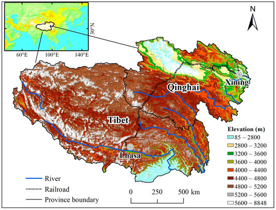
Figure 1.
The geographical location of the Qinghai–Tibet Plateau (QTP).
2.2. Data Source and Pre-Processing
Demographic data for 2000, 2010, and 2016 and contemporary high-resolution covariate datasets were collected for the estimation of the population density of the QTP. Due to the consideration of previous studies [7,33,34] and the data availability, a wide range of factors known to correlate with population density were selected as predictive covariates, including land use/land cover, topography, vegetation productivity, climate pattern, intensity of nighttime lights, road networks, and the locations of POI data (Table 1). In order to make the data from the contemporary covariate datasets match the ancillary input data used for population density estimation, we resampled all datasets to a spatial resolution of 1000 m using the bilinear algorithm, and all datasets were projected in an Albers equal-area projection.

Table 1.
Summary information of the spatial covariate datasets and derived covariates used for the estimation of human population density on the Qinghai–Tibet Plateau (QTP).
2.2.1. Demographic Data and Administrative Unit Boundaries
Demographic counts for 2000 and 2010 on the QTP both at the town-level and county-level were collected from the database of the fifth and sixth census of China, respectively. As the time interval of the national census in China is ten years, the demographic counts in 2016 at the town-level were obtained from the China County Statistical Yearbook (town volume (2017)) in 2017.
The administrative unit boundaries both at the town-level and county-level on the QTP for 2000 were obtained from the Institute of Geographical Sciences and Natural Resources Research [35]. The administrative unit boundary data for 2010 were retrieved from the vector map in 91 Weitu Software. Based on the information on the changes of administrative units in China during 2010–2016 (available at http://www.xzqh.org), the administrative unit boundary data in 2010 were altered to conform with the administrative unit boundaries in 2016. Then, the tabular census data for 2000, 2010, and 2016 were linked to the corresponding administrative units (Figure 2). Due to the lack of town-level administrative unit boundaries for 2000 in 16 counties on the QTP, the missing town-level administrative units were merged and then replaced by county-level administrative boundaries according to previous studies [24,35].
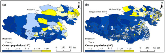
Figure 2.
Maps of the census counts for the QTP at the county level (a) and the town-level (b) matched to their corresponding administrative units for 2010.
2.2.2. Land Use/Land Cover Data
Land use/land cover data for the QTP were obtained from China’s land-use/cover datasets (CLUDs). The datasets have been identified as one of the highest accurate land use/land cover products at the national level for China [36]. These datasets have a spatial resolution of 30 m and provide a long time series from the late 1980s to 2015 at five-year intervals [36,37]. This study used the datasets for 2000, 2010, and 2015. The CLUDs are divided into six land use categories with 25 land use sub-categories. The six categories are cultivated land, forest land, grassland, water body, built-up land, and bare land. Among the six categories and 25 sub-categories of land use, we found a small area of mining land on the QTP, mostly in Qinghai Province, which was classified as built-up land. To improve the accuracy of population mapping, according to the sub-categories of land use, this study initially divided the category of built-up land into built-up areas and mining areas. We then converted each category of land use/land cover data into proportion data at a spatial resolution of 1000 m using the aggregate tool in the ArcGIS software. The proportion data were rescaled by 0 to 100% for each category (Figure 3). Compared with the usual binary classifications of land use/land cover at a resolution of 1000 m, the proportion data with continuous values reserves more detailed spatial information.
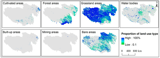
Figure 3.
The proportion of each land use/land cover category on the QTP in 2010.
2.2.3. Geospatial Vector Data
POI data have been increasingly used as ancillary data to improve human population mapping [18,19,20]. The data of rural village POI for 2000 and road networks were obtained from the Institute of Geographical Sciences and Natural Resources Research (IGSNRR). The other POI data including government agencies, tourist destinations, hospitals and clinics, education facilities, and temples, were collected from Baidu Maps (http://map.baidu.com). The POI records from each category were then processed to two types of raster-based derived layers, including a layer with the density of POI and a layer with the Euclidean distance to the nearest geospatial record [7,33,38]. According to existing studies, the layer with the density of POI was generated using the kernel density estimation function in the ArcGIS software [38].
2.2.4. Nighttime Light and Additional Ancillary Data
Nighttime light (NTL) data has been widely used for mapping population density estimation [7,39,40]. The NTL data used in this study included DMSP/OLS NTL data and NPP/VIIRS NTL data. DMSP/OLS data were downloaded from the National Centers for Environmental Information of the National Oceanic and Atmospheric Administration (NOAA) (available at https://ngdc.noaa.gov/eog/dmsp/). The NPP/VIIRS data were downloaded from NOAA/NGDC (available at https://www.ngdc.noaa.gov/eog/viirs/). The DMSP/OLS data were available from 1992 to 2013, while the NPP/VIIRS data were available since 2012. DMSP/OLS data for 2000 and 2010 and NPP/VIIRS data for 2016 were used.
Topographic data were obtained from the United States Geological Survey’s global digital elevation model (DEM). Based on the DEM data, the elevation and slope were extracted. The normalized difference vegetation index (NDVI) datasets from MODIS-Terra (MOD13A2) for the period 2000–2016 were obtained from the National Aeronautics and Space Administration (NASA). To reduce contamination by cloud, snow, and ice cover, we smoothed the annual NDVI cycle using an adaptive Savitzky–Golay approach [41,42]. We then calculated the average NDVI for the growing season for the period 2000–2016. Daily precipitation and temperature records for the QTP and its surrounding areas during 2000–2016 were collected at 315 meteorological stations from the China National Stations’ Fundamental Elements Datasets V3.0. The gridded datasets of growing-season precipitation and temperature at a resolution of 1000 m were interpolated using the ANUSPLIN version 4.2 software.
2.2.5. Other Gridded Population Distribution Datasets
Five global and national gridded population distribution datasets for 2010 with different spatial resolutions were used in this study. Two global datasets were employed, namely the WorldPop dataset (henceforth referred to as WorldPop) and the Gridded Population of the World v4 dataset (hereafter referred to as GPW v4) [7,12]. There are three national datasets for mainland China [11,43,44]. Main covariate datasets for mapping these three datasets are land cover, nighttime light, and elevation data. These five gridded population distribution datasets were created based on the county-level census counts. It should be noted that the Tibet Autonomous Region was excluded in the gridded population distribution dataset from Gaughan et al. (2016, CnPop3) [11]. The aggregate tool in the ArcGIS software was used to upscale the high spatial resolution (e.g., ~100 m) in the data to 1000 m. Summary information of the five population gridded datasets is provided in Table 2.
Table 2.
Summary information of five population gridded datasets for 2010.
2.3. Methods
2.3.1. Random Forest-Based Dasymetric Population Mapping Approach
The RF-based dasymetric population mapping approach is a combination of an RF regression model and a dasymetric population mapping method, and has been successfully used as an underlying model for the estimation of human population density both at national and global scales, due to its excellent performance and generalization capabilities [7,11,38]. In brief, the major processes of this hybrid population mapping approach can be divided into two steps: (1) an RF regression model is initially used to generate a population density weighting layer, which (2) is subsequently applied to dasymetrically redistribute the original census counts within administrative units [7,11].
The general process for RF-based dasymetric population mapping is described in Stevens et al. (2015) [7] and Gaughan et al. (2016) [11]. Several studies have noted that the higher accuracy of predicted population values at the administrative-unit level leads to a higher accuracy of the gridded datasets of population density [14,45]. The town-level (Jiedao/Xiangzhen in Chinese, equivalent to fourth-level administrative units) is the finest administrative unit for which demographic data are publicly released in China; however, it is very difficult to assess the accuracy of the gridded datasets using finer-scale administrative units for census counts. Therefore, in this study, the hybrid population mapping approach was modified to map multi-temporal high-resolution human population density in the QTP. Four steps are outlined in Figure 4. These steps are as follows: (i) fitting the RF model to generate a population density weighting layer using town-level census counts and their corresponding predictive covariates (Figure 5); (ii) dasymetric redistributing of the county-level census counts (see Figure 2a) proportional to the predicted population density weighting layer at the grid-cell level (namely, county-based QTPpop); (iii) comparing the accuracy of the county-based QTPpop with currently available gridded population datasets; and (iv) when the assessment shows that the county-based QTPpop is robust, dasymetric redistributing the town-level census counts (see Figure 2b) proportional to the predicted population density weighting layer at the grid-cell level (namely, town-based QTPpop). According to previous studies [11,29,46], the RF model was used for each census year (2000, 2010, and 2016) to generate multi-temporal gridded datasets of the population density on the QTP, which were subsequently used to detect the changes in population density. The RF model was fitted in the R statistical software using the randomForest package. More details on the parameterization of the RF model can be found in Stevens et al. (2015) [7].
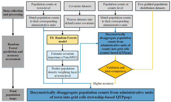
Figure 4.
Flowchart of the disaggregation of population counts from administrative units of towns into 1 km grid cells on the QTP (modified from Stevens et al. [7]).
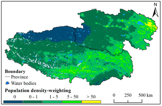
Figure 5.
Population density weighting layer at a spatial resolution of 1 km predicted by the random forest (RF) model for the QTP in 2010.
2.3.2. Technical Validation and Inter-Comparison
(1) Out-of-bag (OOB) error estimation
The out-of-bag (OOB) error estimation, which is an internal cross-validation component of the RF model, provides an accurate and unbiased estimate of the overall accuracy of the RF model [47,48]. During the RF model fitting, one-third of the input data are held in reserve from the bagging iteration process and utilized to obtain an OOB error. The prediction error of the RF model for population density mapping was estimated by averaging the mean squared errors (MSE). Moreover, the OOB error was utilized to evaluate the importance of each model covariate by randomly permutating a given covariate’s OOB data with random noise and computing the percentage increase in the mean squared error (%IncMSE) across all trees of the RF model. Higher values of %IncMSE represent greater variable importance [11].
(2) External Accuracy Assessment
The mapping accuracy is compatible among population density datasets within a given year, nevertheless, the comparisons cannot be reliably performed for datasets from different years [49]. Thus, this study assessed the accuracy of our population density product on the QTP for 2010 by comparing it with five other gridded population datasets (WorldPop, GPW v4, CnPop1, CnPop2, CnPop3) for the same year. The mapping accuracy was assessed via the following steps. First, the county-based QTPpop for 2010 was compared to the town-level census counts by summing gridded population estimates within each town administrative unit. Then, scatter plots of the town-level census count and the town-level estimated population were constructed. The coefficient of determination (R2), root-mean-square error (RMSE), and mean absolute error (MAE) were selected as the statistical measures of mapping accuracy. The same steps were used to assess the accuracy of the five gridded population products.
3. Results
3.1. Accuracy Assessment and Inter-Comparison
The RF model used to predict human population density in the QTP has a consistently high variance explained for 2000, 2010, and 2016, with values of 87.52%, 92.83%, and 91.44%, respectively. The OOB error of the RF model for estimating the town-level-based log of human population density (MSE) for 2000, 2010, and 2016 was 0.21, 0.25, and 0.29, respectively.
The county-based QTPpop for 2010 was highly consistent with the original census counts at the town-level, with an R2 of 0.97 (Figure 6). This value of R2 was higher than those of the five publicly released gridded population density datasets; the R2 value for Worldpop was 0.90, while those of the other four datasets were lower than 0.90, with the lowest value being obtained for GPW v4 (R2 = 0.40). Spatially, the county-based QTPpop better mirrored the characteristics of the population pattern compared to the five publicly available products (Figure 6). First, compared with Cnpop1, CnPop3, and GPW v4, in county-based QTPpop, the phenomenon in which the population density maps displayed abrupt changes along the administrative unit boundaries was mitigated. Second, compared with Cnpop2, in county-based QTPpop, according to the original census counts at the town-level (Figure 2b), the large underestimation of population density in the areas with low population density in the northwestern QTP was mitigated. The county-based QTPpop was more consistent with the WorldPop product than the four other publicly available datasets in terms of the spatial pattern of population distribution on the QTP.
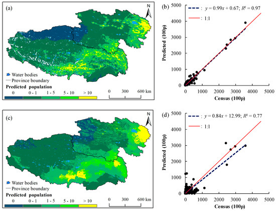
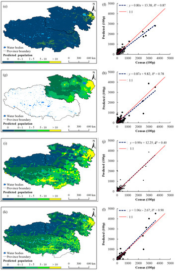
Figure 6.
Comparison of population density maps of the QTP produced using six gridded population datasets for 2010 (a,c,e,g,i,k) and corresponding predicted population unit counts at the town-level compared to the original census counts at the same unit level (b,d,f,h,j,l). (a,b), (c,d), (e,f), (g,h), (i,j), and (k,l) represent the datasets from the county-based QTPpop, Cnpop1, Cnpop2, CnPop3, GPW v4, and WorldPop, respectively. Gridded products denote the population in people per pixel at ~1 km resolution.
Furthermore, the RMSE and MAE of the county-based QTPpop were 4027.23 and 2024.67, respectively, both of which were lower than those of the five publicly available gridded population datasets (Figure 7). Specifically, the RMSE of the county-based QTPpop was about half that of Cnpop1, Cnpop2, WorldPop, and CnPop3, and about one-fifth that of GPW v4. The MAE of the county-based QTPpop was approximately half that of the five publicly available gridded population products except for WorldPop.
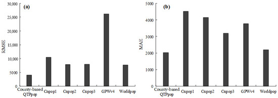
Figure 7.
Comparison of the accuracy statistics ((a) root-mean-square error [RMSE] and (b) mean absolute error [MAE]) of six predicted population density products for 2010.
Internal measures of the accuracy of the RF model and an inter-comparison of external accuracy assessments among the five recently released gridded population datasets indicated that the county-based QTPpop yielded a higher mapping accuracy compared to the five other products. One important explanation is that the use of fine-scale administrative units for census counts improved the model’s ability for population mapping. As above-mentioned, the accuracy of the population density dataset based on county-level census counts was higher than those of the five publicly available population density products. Meanwhile, the town-level was the finest statistical unit in publicly released demographic data for China, and the town-based QTPpop took full advantage of the spatially detailed town population counts. It is reasonable to expect that the town-based QTPpop can yield higher accuracy than the county-based QTPpop. More interpretation is given in Section 4.1. Thus, we used the town-based QTPpop in subsequent analyses.
3.2. Importance of Variables in Explaining Population Density
The relative importance of variables in explaining population density on the QTP is shown in Figure 8. Of the 24 variables used in the RF model, the 10 that contributed most to the estimation of population density can be subdivided into three categories: (1) six POI-related variables; (2) two land-use related variables; and (3) variables related to topographical features and vegetation productivity. The variable “Distance to Temples” has the largest contribution to the prediction of population density. This variable is closely related to the religious beliefs of inhabitants across the QTP. Aside from this variable, the two variables that contributed the most to the prediction of population density were “Density of Villages” and “Elevation”. The fact that elevation is among the top three variables is understandable since most inhabitants on the QTP live in areas with relatively low elevation such as valleys. The “Density of Villages” and “Distance to Villages” variables were good measures of population density in the QTP. Meanwhile, the importance of the variable “Percentage of Cultivated Areas” was greater than that of “Percentage of Built-up Areas”, which may be related to the low level of urbanization across the QTP and the fact that the population density of farmers depends on the distribution of cultivated areas. Surprisingly, the importance of the “Night-lights’ intensity” variable was outside the top 10, likely due to the low level of urbanization in the study area.
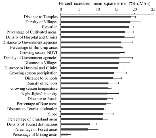
Figure 8.
Percentage-increased mean squared errors (%IncMSE) indicating the importance of variables in explaining the population density in the RF model.
3.3. Spatio-Temporal Change of Human Population Density on the QTP
The town-based QTPpop provided an accurate description of the population density on the QTP in 2000, 2010, and 2016 (Figure 9). Overall, the QTP has a sparse population distribution. In about 14% of the QTP, the population density is zero; these areas are mainly distributed around the Kunlun Mountains and Altun Mountains, including the north of the Tibet Autonomous Region and western Kekexili, Qinghai. Areas with relatively high population density are primarily located in the Yellow River–Huangshui River Valley and the Yarlung Zangbo and Lhasa River Valley.
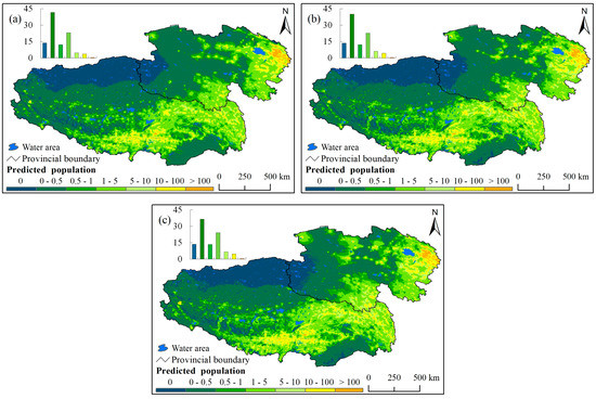
Figure 9.
Gridded population maps of the QTP for (a) 2000, (b) 2010, and (c) 2016.
From 2000 to 2016, the extreme sparsely populated areas in the QTP gradually decreased while the relatively densely populated area rapidly increased (Figure 9). The proportion of areas with a population density of less than 0.5 persons/km2 decreased from 41.62% in 2000 to 40.23% in 2010 to 36.52% in 2016. In contrast, the proportion of areas with a population density between 5 and 10 persons/km2 increased from 4.82% in 2000 to 6.25% in 2010 to 6.70% in 2016, while the proportion of areas with a population density of above 10 persons/km2 increased from 4.26% in 2000 to 4.91% in 2010 to 5.35% in 2016.
The areas in which the population growth between 2000 and 2016 exceeded 0.1 persons/km2, accounting for 42.81% of the total area of the QTP, mainly distributed in the eastern and southern parts of Qinghai Province and the central-eastern parts of the Tibet Autonomous Region (Figure 10c). The proportion of areas with population growth between 2 and 5 persons/km2 and above 5 persons/km2 were 5.14% and 2.57%, respectively. In contrast, the areas with a population decrease above 0.1 persons/km2 accounted for 15.71% of the total area, and were mainly distributed in agricultural and pastoral areas around relatively densely populated areas. Additionally, in both the periods of 2000–2010 and 2010–2016, the areas with increased population density tended to be areas with higher population density, while the areas with unchanged or lower population density were mainly located in more sparsely populated areas (Figure 10a,b).
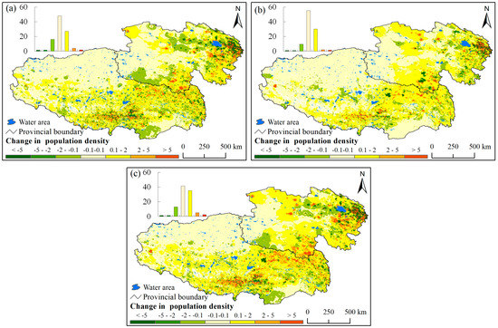
Figure 10.
Variation in the population density of the QTP during the periods of (a) 2000–2010, (b) 2010–2016, and (c) 2000–2016.
4. Discussion
4.1. Advancement Using Town-Level Population Counts in Population Mapping for the QTP
In this study, a detailed multi-temporal human population distribution dataset was generated for the QTP based on town-level population counts. A comparison with five existing national and global gridded population products for 2010 indicated that our new population products more accurately characterized the human population distribution in the QTP (Figure 6 and Figure 7). In this work, the higher accuracy of the population density weighting layer was initially predicted using the RF model based on the town-level population counts. Previous studies have noted that the choice of finer census units generally leads to a larger range of measured population densities and better reflects geographic variation in population, which can minimize the span of the model’s spatial-scale conversion [12,25,45]. Meanwhile, the dasymetric redistribution of lower population counts in finer administrative units using the predicted population density weighting layer can reduce the error in the final human population density datasets [45]. Therefore, compared with the county-based QTPpop, the town-based QTPpop had a higher accuracy.
The size of administrative units at the same hierarchy of China exhibited considerable differences over the QTP [16], with the size of administrative units of lower hierarchy being much larger than that of higher hierarchy (Figure 2). This phenomenon may introduce uncertainties in human population mapping when the population counts with the higher level of administrative units are used. In the following, Golmud County (located in western Qinghai Province) is taken as an example. This county consists of two unconnected parts, namely Tanggulashan Town and other areas. Tanggulashan Town has a low population density, while other areas in Golmud County have a higher population density (Figure 2). Some of the currently released population products analyzed in the present stud greatly overestimate the population in Tanggulashan Town, which were mapped based on the county-level census (Figure 6c,g). Similar phenomena also occurs in the northwestern QTP (Figure 6).
4.2. Effectiveness of Local Population-Sensitive Points-of-Interest (POIs) for Improving Population Mapping in Remote Rural Areas
Detailed covariates have been shown to improve the accuracy of models of population density [7]. This study used population-sensitive POI data as input variables in the RF regression model, which improved the accuracy of the estimation of the human population density in the QTP. It was found that of the 10 variables that were most important for explaining population density, six were POI-related variables such as “Distance to Temples”, “Density of Villages”, and “Distance to Villages”. This result indicates that, for the mapping of the population density of the QTP, it is necessary to introduce local social and cultural variables as well as physical variables (e.g., topographical features) [35,50]. In contrast, although the intensity of nighttime lights has been considered as an excellent predictor of urban population density [16,17], the importance of the variable “Night-lights’ intensity” may significantly weaken in low- and middle-income regions, especially in remote rural areas such as the QTP.
The town-based QTPpop product that was constructed in this study consisted of temporally comparable population datasets based on demographic data for 2000, 2010, and 2016 and a number of covariates that are time-invariant and temporally explicit. Compared with national population datasets (e.g., Xu et al. (2017) [43], Gaughan et al. (2016) [11], and Tan et al. (2018) [16]), we not only used variables related to built-up areas and night-light intensity to reconstruct the changes in population distribution over time, but also employed population-sensitive POIs variables (e.g., distances to temples and settlements) as predictors of population distribution in remote rural areas.
4.3. Population Growth on the QTP
The results of this study suggest that between 2000 and 2016, the QTP experienced a reduction in areas with extremely low population density. This is contrary to the results of a study that found that, in mainland China, between 2000 and 2016, there was an overall expansion of areas with low population density [16]. One potential explanation for this is that the level of urbanization on the QTP is much lower than that in Central and Eastern China. The results of the present study indicate that in rural areas of the QTP, about half of the total area showed an increase in population density, which may increase human pressures on this world’s largest pastoral alpine ecosystem [51]. Up to now, more than 150 nature reserves have been created on the QTP, which account for one-third of its total area [52]. Furthermore, since 2004, an ecological restoration project called the Grazing Withdrawal Program (GWP) has been implemented to restore the grassland ecosystems of the QTP. The widespread population growth on the QTP may offset the effectiveness of its nature reserves and the GWP. Therefore, more attention should be paid to coordinating population growth and the preservation of the fragile ecological environment of the QTP, especially in nature reserves.
4.4. Limitations and the Future Research
This work provides a case study of population density mapping in remote rural areas based on a RF model. Even though the accuracy of our newly products were higher than five publicly released national or global gridded population products, recent studies noted that deep learning could achieve a higher accuracy of population mapping than the shallow machine learning [53]. Meanwhile, with the improvement in the geospatial big data of POIs and the location-based social media data, more attention should be paid to improving the accuracy of human population mapping in remote rural areas in future work [1], especially for temporally comparable population datasets.
5. Conclusions
In this study, the temporal and spatial change of human population density on the QTP from 2000 to 2016 was estimated based on demographic data at the town-level, remotely sensed data, and local population-sensitive POI data. The results indicated that our new population map exhibited higher accuracy compared with five recently released gridded population density datasets. Both the root-mean-square error and the mean absolute error for our map were about half of those of the compared products (with the exception of the WorldPop). The higher accuracy of our new population map largely depended on taking advantage of the finer scale demographic count and local population-sensitive POIs. POI-related variables (e.g., “Distance to Temples” and “Density of Villages”) were more important for explaining population density on the QTP than the variable “Night-lights’ intensity”. Furthermore, in large areas of the northern QTP, accounting for about 14% of the total area of the QTP, population density was zero. About half of the QTP showed a rapid increase in population density from 2000 to 2016, mainly located in the eastern and southern parts of Qinghai Province and the central-eastern parts of the Tibet Autonomous Region.
Author Contributions
Conceptualization, L.L. (Linshan Liu) and Y.Z.; Methodology, L.L. (Lanhui Li), H.Z.; writing—original draft preparation, L.L. (Lanhui Li); Writing—review and editing, Y.Z., L.L. (Linshan Liu), Z.W., S.L., and M.D. All authors have read and agreed to the published version of the manuscript.
Funding
This research was funded by the National Natural Science Foundation of China (Grant No. 41671104), the second Tibetan Plateau Scientific Expedition and Research Program (Grant No. 2019QZKK0603), the Strategic Priority Research Program of Chinese Academy of Sciences (Grant No. XDA20040201), and the Research Program of Xiamen University Technology (Grant No. YKJ190).
Acknowledgments
We sincerely thank Xuchao Yang from Zhejiang University and Tingting Ye from Monash University for their valuable feedback.
Conflicts of Interest
The authors declare no conflict of interest.
References
- Leyk, S.; Gaughan, A.E.; Adamo, S.B.; de Sherbinin, A.; Balk, D.; Freire, S.; Rose, A.; Stevens, F.R.; Blankespoor, B.; Frye, C.; et al. The spatial allocation of population: A review of large-scale gridded population data products and their fitness for use. Earth Syst. Sci. Data 2019, 11, 1385–1409. [Google Scholar] [CrossRef]
- Small, C.; Cohen, J. Continental Physiography, Climate, and the Global Distribution of Human Population. Curr. Anthropol. 2004, 45, 269–277. [Google Scholar] [CrossRef]
- McGowan, P.J.K. Mapping the terrestrial human footprint. Nature 2016, 537, 172–173. [Google Scholar] [CrossRef] [PubMed]
- United Nations. Concise Report on the World Population Situation 2014. Secretaría de la ONU. D. o. E. a. 2014. p. 2. Available online: https://www.un.org/en/development/desa/population/publications/pdf/trends/Concise%20Report%20on%20the%20World%20Population%20Situation%202014/en.pdf (accessed on 3 December 2020).
- Balk, D.L.; Deichmann, U.; Yetman, G.; Pozzi, F.; Hay, S.I.; Nelson, A. Determining Global Population Distribution: Methods, Applications and Data. Adv. Parasit. 2006, 62, 119–156. [Google Scholar]
- Wardrop, N.A.; Jochem, W.C.; Bird, T.J.; Chamberlain, H.R.; Clarke, D.; Kerr, D.; Bengtsson, L.; Juran, S.; Seaman, V.; Tatem, A.J. Spatially disaggregated population estimates in the absence of national population and housing census data. Proc. Natl. Acad. Sci. USA 2018, 115, 3529–3537. [Google Scholar] [CrossRef]
- Stevens, F.R.; Gaughan, A.E.; Linard, C.; Tatem, A.J. Disaggregating Census Data for Population Mapping Using Random Forests with Remotely-Sensed and Ancillary Data. PLoS ONE 2015, 10, e107042. [Google Scholar] [CrossRef]
- Zeng, C.; Zhou, Y.; Wang, S.; Yan, F.; Zhao, Q. Population spatialization in China based on night-time imagery and land use data. Int. J. Remote Sens. 2011, 32, 9599–9620. [Google Scholar] [CrossRef]
- Yao, Y.; Liu, X.; Li, X.; Zhang, J.; Liang, Z.; Mai, K.; Zhang, Y. Mapping fine-scale population distributions at the building level by integrating multisource geospatial big data. Int. J. Geogr. Inf. Sci. 2017, 31, 1220–1244. [Google Scholar] [CrossRef]
- Wu, S.; Qiu, X.; Wang, L. Population Estimation Methods in GIS and Remote Sensing: A Review. GISci. Remote Sens. 2005, 42, 80–96. [Google Scholar] [CrossRef]
- Gaughan, A.E.; Stevens, F.R.; Huang, Z.; Nieves, J.J.; Sorichetta, A.; Lai, S.; Ye, X.; Linard, C.; Hornby, G.M.; Hay, S.I.; et al. Spatiotemporal patterns of population in mainland China, 1990 to 2010. Sci. Data 2016, 3, 160005. [Google Scholar] [CrossRef]
- Doxsey-Whitfield, E.; MacManus, K.; Adamo, S.B.; Pistolesi, L.; Squires, J.; Borkovska, O.; Baptista, S.R. Taking Advantage of the Improved Availability of Census Data: A First Look at the Gridded Population of the World, Version 4. Pap. Appl. Geogr. 2015, 1, 226–234. [Google Scholar] [CrossRef]
- Reed, F.; Gaughan, A.; Stevens, F.; Yetman, G.; Sorichetta, A.; Tatem, A. Gridded Population Maps Informed by Different Built Settlement Products. Data 2018, 3, 33. [Google Scholar] [CrossRef]
- Sorichetta, A.; Hornby, G.M.; Stevens, F.R.; Gaughan, A.E.; Linard, C.; Tatem, A.J. High-resolution gridded population datasets for Latin America and the Caribbean in 2010, 2015, and 2020. Sci. Data 2015, 2, 150045. [Google Scholar] [CrossRef] [PubMed]
- Sutton, P. Modeling population density with night-time satellite imagery and GIS. Comput. Environ. Urban Syst. 1997, 21, 227–244. [Google Scholar] [CrossRef]
- Tan, M.; Li, X.; Li, S.; Xin, L.; Wang, X.; Li, Q.; Li, W.; Li, Y.; Xiang, W. Modeling population density based on nighttime light images and land use data in China. Appl. Geogr. 2018, 90, 239–247. [Google Scholar] [CrossRef]
- Li, X.; Zhou, W. Dasymetric mapping of urban population in China based on radiance corrected DMSP-OLS nighttime light and land cover data. Sci. Total Environ. 2018, 643, 1248–1256. [Google Scholar] [CrossRef] [PubMed]
- Yang, X.; Ye, T.; Zhao, N.; Chen, Q.; Yue, W.; Qi, J.; Zeng, B.; Jia, P. Population Mapping with Multisensor Remote Sensing Images and Point-Of-Interest Data. Remote Sens. 2019, 11, 574. [Google Scholar] [CrossRef]
- Bakillah, M.; Liang, S.; Mobasheri, A.; Jokar Arsanjani, J.; Zipf, A. Fine-resolution population mapping using OpenStreetMap points-of-interest. Int. J. Geogr. Inf. Sci. 2014, 28, 1940–1963. [Google Scholar] [CrossRef]
- Zhao, Y.; Li, Q.; Zhang, Y.; Du, X. Improving the Accuracy of Fine-Grained Population Mapping Using Population-Sensitive POIs. Remote Sens. 2019, 11, 2502. [Google Scholar] [CrossRef]
- Hoffman-Hall, A.; Loboda, T.V.; Hall, J.V.; Carroll, M.L.; Chen, D. Mapping remote rural settlements at 30 m spatial resolution using geospatial data-fusion. Remote Sens. Environ. 2019, 233, 111386. [Google Scholar] [CrossRef]
- Miehe, G.; Schleuss, P.; Seeber, E.; Babel, W.; Biermann, T.; Braendle, M.; Chen, F.; Coners, H.; Foken, T.; Gerken, T.; et al. The Kobresia pygmaea ecosystem of the Tibetan highlands-Origin, functioning and degradation of the world’s largest pastoral alpine ecosystem. Sci. Total Environ. 2019, 648, 754–771. [Google Scholar] [CrossRef]
- Sun, H.; Zheng, D.; Tandong, Y.; Zhang, Y. Protection and construction of the national ecological security shelter zone on Tibetan Plateau. Acta Geogr. Sin. 2012, 1, 12–13. [Google Scholar]
- Wang, C.; Kan, A.; Zeng, Y.; Li, G.; Wang, M.; Ci, R. Population distribution pattern and influencing factors in Tibet based on random forest model. Acta Geogr. Sin. 2019, 74, 664–680. [Google Scholar]
- Shunbao, L.; Zehui, L. Study on spatialization of population census data based on relationship between population distribution and land use: Taking Tibet as an example. J. Nat. Resour. 2003, 18, 659–665. [Google Scholar]
- Li, S.; Zhang, Y.; Wang, Z.; Li, L. Mapping human influence intensity in the Tibetan Plateau for conservation of ecological service functions. Ecosyst. Serv. 2018, 30, 276–286. [Google Scholar] [CrossRef]
- Nan, D.; Xiaohuan, Y.; Hongyan, C. Research progress and perspective on the spatialization of population data. J. Geo -Inform. Sci. 2016, 18, 1295–1304. [Google Scholar]
- Bai, Z.; Wang, J.; Wang, M.; Gao, M.; Sun, J. Accuracy Assessment of Multi-Source Gridded Population Distribution Datasets in China. Sustainability 2018, 10, 1363. [Google Scholar] [CrossRef]
- Linard, C.; Kabaria, C.W.; Gilbert, M.; Tatem, A.J.; Gaughan, A.E.; Stevens, F.R.; Sorichetta, A.; Noor, A.M.; Snow, R.W. Modelling changing population distributions: An example of the Kenyan Coast, 1979–2009. Int. J. Digit. Earth 2017, 10, 1017–1029. [Google Scholar] [CrossRef]
- Zhao, T.; Song, B.; Chen, Y.; Yan, H.; Xu, Z. Analysis of Population Distribution and Its Spatial Relationship with Terrain Elements in the Yarlung Zangbo River, Nyangqu River and Lhasa River Region, Tibet. J. Geo -Inform. Sci. 2017, 19, 225–237. [Google Scholar]
- Chen, F.; Welker, F.; Shen, C.; Bailey, S.E.; Bergmann, I.; Davis, S.; Xia, H.; Wang, H.; Fischer, R.; Freidline, S.E.; et al. A late Middle Pleistocene Denisovan mandible from the Tibetan Plateau. Nature 2019, 569, 409–412. [Google Scholar] [CrossRef]
- Allan, J.R.; Venter, O.; Watson, J.E.M. Temporally inter-comparable maps of terrestrial wilderness and the Last of the Wild. Sci. Data 2017, 4, 170187. [Google Scholar] [CrossRef]
- Nieves, J.J.; Stevens, F.R.; Gaughan, A.E.; Linard, C.; Sorichetta, A.; Hornby, G.; Patel, N.N.; Tatem, A.J. Examining the correlates and drivers of human population distributions across low- and middle-income countries. J. R. Soc. Interface 2017, 14, 20170401. [Google Scholar] [CrossRef] [PubMed]
- Patel, N.N.; Stevens, F.R.; Huang, Z.; Gaughan, A.E.; Elyazar, I.; Tatem, A.J. Improving Large Area Population Mapping Using Geotweet Densities. Trans. GIS 2017, 21, 317–331. [Google Scholar] [CrossRef] [PubMed]
- Bai, Z.; Wang, J.; Yang, Y.; Sun, J. Characterizing spatial patterns of population distribution at township level across the 25 provinces in China. Acta Geogr. Sin. 2015, 70, 1229–1242. [Google Scholar]
- Liu, J.; Kuang, W.; Zhang, Z.; Xu, X.; Qin, Y.; Ning, J.; Zhou, W.; Zhang, S.; Li, R.; Yan, C.; et al. Spatiotemporal characteristics, patterns, and causes of land-use changes in China since the late 1980s. J. Geogr. Sci. 2014, 24, 195–210. [Google Scholar] [CrossRef]
- Kuang, W. A 30-m resolution national urban land-cover dataset of China, 2000–2015. Earth Syst. Sci. Data Discuss. 2019, 1–33. Available online: https://essd.copernicus.org/preprints/essd-2019-65/essd-2019-65.pdf (accessed on 3 December 2020).
- Ye, T.; Zhao, N.; Yang, X.; Ouyang, Z.; Liu, X.; Chen, Q.; Hu, K.; Yue, W.; Qi, J.; Li, Z.; et al. Improved population mapping for China using remotely sensed and points-of-interest data within a random forests model. Sci. Total Environ. 2019, 658, 936–946. [Google Scholar] [CrossRef] [PubMed]
- Shi, K.; Yu, B.; Huang, Y.; Hu, Y.; Yin, B.; Chen, Z.; Chen, L.; Wu, J. Evaluating the Ability of NPP-VIIRS Nighttime Light Data to Estimate the Gross Domestic Product and the Electric Power Consumption of China at Multiple Scales: A Comparison with DMSP-OLS Data. Remote Sens. 2014, 6, 1705–1724. [Google Scholar] [CrossRef]
- Elvidge, C.D.; Baugh, K.E.; Dietz, J.B.; Bland, T.; Sutton, P.C.; Kroehl, H.W. Radiance Calibration of DMSP-OLS Low-Light Imaging Data of Human Settlements. Remote Sens. Environ. 1999, 68, 77–88. [Google Scholar] [CrossRef]
- Jönsson, P.; Eklundh, L. TIMESAT—A program for analyzing time-series of satellite sensor data. Comput. Geosci. UK 2004, 30, 833–845. [Google Scholar] [CrossRef]
- Chen, J.; Jönsson, P.; Tamura, M.; Gu, Z.; Matsushita, B.; Eklundh, L. A simple method for reconstructing a high-quality NDVI time-series data set based on the Savitzk-Golay filter. Remote Sens. Environ. 2004, 91, 332–344. [Google Scholar] [CrossRef]
- Xu, X. China Population Spatial Distribution Kilometer Grid Dataset. In Data Registration and Publishing System of Resource and Environmental Science Data Center of Chinese Academy of Sciences; 2017; Available online: http://www.resdc.cn/DOI/DOI.aspx?DOIid=32. (accessed on 3 December 2020).
- Fu, J.Y.; Jiang, D.; Huang, Y.H. 1-km Gridded Population Dataset of China (2005, 2010). Glob. Chang. Res. Data Publ. Repos. 2014. [Google Scholar] [CrossRef]
- Gaughan, A.E.; Stevens, F.R.; Linard, C.; Patel, N.N.; Tatem, A.J. Exploring nationally and regionally defined models for large area population mapping. Int. J. Digit. Earth 2016, 8, 989–1006. [Google Scholar] [CrossRef]
- Lloyd, C.T.; Chamberlain, H.; Kerr, D.; Yetman, G.; Pistolesi, L.; Stevens, F.R.; Gaughan, A.E.; Nieves, J.J.; Hornby, G.; MacManus, K.; et al. Global spatio-temporally harmonised datasets for producing high-resolution gridded population distribution datasets. Big Earth Data 2019, 3, 108–139. [Google Scholar] [CrossRef]
- Breiman, L. Random forests. Mach. Learn. 2001, 45, 1–5. [Google Scholar]
- Liaw, A.W.M. Classification and Regression by RandomForest. R News 2002, 2, 18–22. [Google Scholar]
- Zoraghein, H.; Leyk, S. Data-enriched interpolation for temporally consistent population compositions. GISci. Remote Sens. 2018, 56, 430–461. [Google Scholar] [CrossRef]
- Liao, S.; Sun, J. GIS based spatialization of population census data in Qinghai-Tibet Plateau. Acta Geogr. Sin. 2003, 58, 25–33. [Google Scholar]
- Qi, W.; Liu, S.; Zhou, L. Regional differentiation of population in Tibetan Plateau: Insight from the “Hu Line”. Acta Geogr. Sin. 2020, 75, 255–267. [Google Scholar]
- Zhang, Y.; Hu, Z.; Qi, W.; Wu, X.; Bai, W.; Li, L.; Ding, M.; Liu, L.; Wang, Z.; Zheng, D. Assessment of effectiveness of nature reserves on the Tibetan Plateau based on net primary production and the large sample comparison method. J. Geogr. Sci. 2016, 26, 27–44. [Google Scholar] [CrossRef]
- Zhao, S.; Liu, Y.; Zhang, R.; Fu, B. China’s population spatialization based on three machine learning models. J. Clean. Prod. 2020, 256, 120644. [Google Scholar] [CrossRef]
Publisher’s Note: MDPI stays neutral with regard to jurisdictional claims in published maps and institutional affiliations. |
© 2020 by the authors. Licensee MDPI, Basel, Switzerland. This article is an open access article distributed under the terms and conditions of the Creative Commons Attribution (CC BY) license (http://creativecommons.org/licenses/by/4.0/).