Abstract
Collapsed buildings should be detected with the highest priority during earthquake emergency response, due to the associated fatality rates. Although deep learning-based damage detection using vertical aerial images can achieve high performance, as depth information cannot be obtained, it is difficult to detect collapsed buildings when their roofs are not heavily damaged. Airborne LiDAR can efficiently obtain the 3D geometries of buildings (in the form of point clouds) and thus has greater potential to detect various collapsed buildings. However, there have been few previous studies on deep learning-based damage detection using point cloud data, due to a lack of large-scale datasets. Therefore, in this paper, we aim to develop a dataset tailored to point cloud-based building damage detection, in order to investigate the potential of point cloud data in collapsed building detection. Two types of building data are created: building roof and building patch, which contains the building and its surroundings. Comprehensive experiments are conducted under various data availability scenarios (pre–post-building patch, post-building roof, and post-building patch) with varying reference data. The pre–post scenario tries to detect damage using pre-event and post-event data, whereas post-building patch and roof only use post-event data. Damage detection is implemented using both basic and modern 3D point cloud-based deep learning algorithms. To adapt a single-input network, which can only accept one building’s data for a prediction, to the pre–post (double-input) scenario, a general extension framework is proposed. Moreover, a simple visual explanation method is proposed, in order to conduct sensitivity analyses for validating the reliability of model decisions under the post-only scenario. Finally, the generalization ability of the proposed approach is tested using buildings with different architectural styles acquired by a distinct sensor. The results show that point cloud-based methods can achieve high accuracy and are robust under training data reduction. The sensitivity analysis reveals that the trained models are able to locate roof deformations precisely, but have difficulty recognizing global damage, such as that relating to the roof inclination. Additionally, it is revealed that the model decisions are overly dependent on debris-like objects when surroundings information is available, which leads to misclassifications. By training on the developed dataset, the model can achieve moderate accuracy on another dataset with different architectural styles without additional training.
1. Introduction
Building damage detection is a crucial task after large-scale natural disasters, such as earthquakes, as it can provide vital information for humanitarian assistance and post-disaster recovery. Remotely sensed images are often used for earthquake-induced damage mapping, due to their ability to cover a wide range in a short time period [1,2]. In general, there are two types of approaches, which are adopted according to the availability of data. The first type is change detection approaches, which compare pre- and post-event images, whereas the second type is solely based on post-event images [3]. The former can usually achieve higher performance, but the latter is often preferred, as the acquisition of pre-event data is not always guaranteed.
Boosted by the rapid development of computer vision and machine learning technologies, more and more damage detection methods using supervised learning—through training and testing using large-scale datasets—have been developed [4,5]. Among machine learning algorithms, deep learning [6] is a rapidly developing technology that can dramatically outperform previous conventional methods for image processing [7]. The strength of deep learning lies in the automatically optimized feature extraction process, which is often manually carried out by human experts in conventional machine learning pipelines. The success of deep learning has also led to an increased interest in applying deep neural networks (DNNs) to large-scale building damage detection using vertical aerial images [8], where their performance has been proven to be superior to that of conventional supervised learning approaches [9]. Trained DNNs are able to classify building damage by learning the patterns of roof failure, as well as the surrounding objects (e.g., debris, collapsed walls). Despite their state-of-the-art performance, fundamental limitations with respect to image-based approaches have also been reported. For instance, story-collapsed buildings with slight roof failures are extremely hard to identify merely by vertical images [10], as shown in Figure 1. This is due to a lack of 3D geometric information of buildings revealed in vertical 2D images. This is extremely problematic as the partial or complete collapse of a building may greatly endanger its residents [11], and thus, they should be detected with the highest priority. Therefore, the use of technology that is more suitable for the detection of collapsed buildings needs to be introduced.
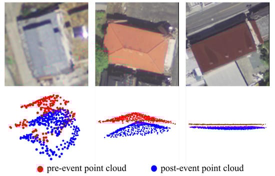
Figure 1.
Examples of collapsed buildings that are hard to detect in vertical images. Aerial images were provided by [12].
Airborne light detection and ranging (LiDAR) systems are capable of rapidly obtaining position and precise elevation information in the form of 3D point cloud data. These systems can operate under most weather conditions by using the active sensing principle, making them an attractive choice for building damage detection. As can be observed in Figure 1, the obtained point cloud can successfully capture the deformations of buildings, which are hardly visible in vertical aerial images. Therefore, LiDAR technology has greater potential, being able to obtain more precise height information than vertical images, to detect severely damaged (e.g., story-collapsed) buildings. Similar to image-based methods, multi-temporal change detection [13], as well as single-temporal approaches [14] have been used to assess building damage using LiDAR point clouds. As buildings are often represented by roofs (the other parts are normally not visible or partially visible for lower residential buildings) in airborne LiDAR point cloud data, a large number of methods have been proposed to detect surface and structural damages represented by roofs. For instance, region-growing-based methods are proposed to detect the planes by segmenting 2.5D raster data and subsequently classified by comparing post-event data with pre-event wireframe reference building models [15,16]. However, these approaches require multiple parameter-sensitive algorithms for detecting planes and roofs, which make them time-consuming to generate optimal results. Furthermore, the constant values of parameters in segmentation process are vulnerable to non-uniform density and data corruption. Structural damages such as roof inclinations can be reliably detected by calculating angle between geometric axis of roofs and vertical planes [17]. However, the method put strong assumptions on the type of building roofs, and hence this type of method is not suitable for large areas with varying roof types. Some approaches utilize radiometric information of (oblique) images to assist the building damage detection in the 3D domain [18,19]. Nevertheless, oblique image-based approaches are difficult to adapt to dense residential areas with low-height buildings because of the large numbers of occlusions. Moreover, rich radiometric information from images is not always available to assist 3D building damage detection.
Damage detection using vertical aerial images in deep learning has achieved satisfactory results so far. Following its success, 3D deep learning on point cloud data for damage assessment should therefore naturally be promising and worthy of investigation. Indeed, the seminal work of PointNet [20] and its variants [21,22,23], which directly operate on point clouds, have demonstrated superior performance compared to conventional feature-engineering-based approaches [20], as well as DNNs, which require additional input conversions [24,25]. The comprehensive review of recent development of point cloud-based deep learning including proposed algorithms, benchmark datasets, and applications on various 3D vision tasks were provided by [26]. Despite the remarkable progress of 3D point cloud-based DNNs, to the best of our knowledge, based on the screening of the recent literature, it is apparent that only a limited number of studies exist regarding the use of 3D deep learning for point cloud-based building damage detection. The inferred primary reason for the limited number of works is the absence of a large-scale airborne LiDAR dataset tailored to 3D building damage detection. Although an SfM-based point cloud dataset was developed and the performance of 3D voxel-based DNN was tested using the developed dataset in [27], the size of the dataset developed was relatively small. A large-scale dataset is a crucial and fundamental resource for developing advanced algorithms for targeted tasks, as well as for providing training and benchmarking data for such algorithms [28,29,30,31], which requires decent expertise and can be labor-intensive.
To this end, this study aims to reveal the potential and current limitations of 3D point cloud-based deep learning approaches for building damage detection by creating a dataset tailored to the targeted task. Two types of building data were created: building roof and building patch, which contains a building and its surroundings. Furthermore, mainstream algorithms are used to evaluate its performance by using the developed dataset under varying data availability scenarios (pre–post-building patch, post-building roof, and post-building patch) and reference data. The pre–post scenario tries to detect damage using pre-event and post-event data, whereas post-building patch and roof only use post-event data. In addition, to validate whether the developed model can gain correct knowledge about problem representations, a sensitivity analysis is conducted, considering the nature of building damages. The robustness of the trained models against sample reduction is tested by conducting an ablation study. Finally, the generalization ability of the trained model is examined using LiDAR data obtained with a different airborne sensor. The building point cloud obtained by this sensor has a different point density, and the architectural style (reinforced concrete) of these data is distinctly different, compared to the in the proposed dataset (wooden).
To summarize, this paper provides the following contributions:
- We create a large-scale point cloud dataset tailored to building damage detection using deep learning approaches.
- We perform damage detection under three data availability scenarios: pre–post, post-building patch, and building roof. The obtained individual results are quantitatively analyzed and compared.
- We propose a general extension framework that extends single-input networks, which accept a single building point clouds, to the pre–post (i.e., two building point clouds) scenario.
- We propose a visual explanation method to validate the reliability of the trained models through a sensitivity analysis under the post-only scenario.
- We validate the generalization ability of models trained using the created dataset by applying the pre-trained models to data having distinct architectural styles captured by a distinct sensor.
The remainder of this paper is organized as follows: Section 2 details the procedures of dataset creation. Section 3 introduces the damage detection framework and the experimental setting. Section 4 presents the experimental results followed by discussions in Section 5. The conclusions are presented in Section 6, providing a brief summary of our findings and prospects for future studies.
2. Dataset Creation
In this section, the LiDAR data and field survey data used for creating the dataset are introduced. The study area selected in this study is Mashiki Town in Kumamoto Prefecture, Japan. Mashiki Town was severely damaged by the 2016 Kumamoto Earthquakes. Specifically, we chose the central area of Mashiki—which is shown as the red shaded region in Figure 2—as the target area to create the dataset. Buildings in the surveyed regions were densely distributed, with most of them constructed using wooden materials. The point cloud data in Mashiki Town were extracted using vector data provided by the Geospatial Information Authority (GSI) of Japan. The residential buildings were first located by GPS coordinates obtained from a field survey and automatically extracted for further manual annotation. All the processing and analysis steps were implemented in Python and QGIS [32].
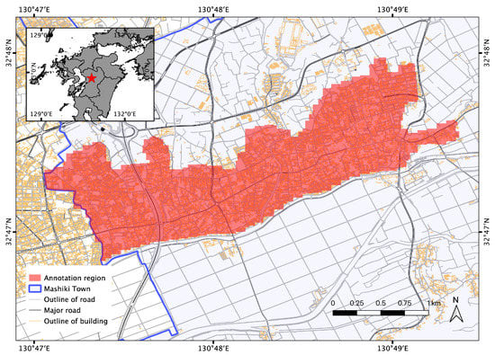
Figure 2.
The central area of Mashiki Town is chosen as the study area of this study, which is shown as the red shaded area. The residential buildings in this area were densely distributed and severely damaged by the 2016 Kumamoto Earthquake.
2.1. Data Source
2.1.1. LiDAR
During 14–16 April 2016, a series of earthquakes struck Kumamoto Prefecture, Japan. The foreshock of 6.2 occurred on 14 April, followed by the mainshock of 7.0 on 16 April. The pre-mainshock LiDAR dataset [33] was acquired on 15 April 2016, and the post-mainshock LiDAR dataset was acquired on 23 April 2016 [34] by Asia Air Survey Co., Ltd. (Chiba, Japan), covering the western half of the rupture zone. Two surveys were conducted, with identical equipment and other conditions, which generated average point densities of 1.5–2 points/m2 and 3–4 points/m2 (scanned twice), respectively [13]. For clarity, the pre-mainshock LiDAR data are called pre-event LiDAR, while the post-mainshock data are called post-event LiDAR in this study.
2.1.2. Field Survey
After the mainshock, the local governments of Kumamoto Prefecture conducted a series of field surveys for assessing the building damage, according to the “operational guideline for damage assessment of residential buildings in disasters” issued by the Cabinet Office of Japan [35]. If a building was recognized as destroyed (not necessarily collapsed), the type of collapse (i.e., story-collapse or not) was determined by the field investigators [36]. Photographs of the target building were taken by investigators, and the building GPS coordinates were recorded. The information collected in the field surveys used in this study included the damage grade, photographs, and GPS coordinates of the surveyed buildings.
2.2. Procedures of Dataset Creation
2.2.1. Information Extraction
As shown in the Figure 3, the first step to create the dataset was to extract the damage information. Damage grades and descriptions, as well as the collapse type were collected during field surveys using recording sheets. Simplified recording sheet is shown in Figure 4. The original recording sheet made by the Cabinet Office of Japan is available online [37]. These recording sheets were digitized by investigators and stored with photographs taken during the surveys. In order to extract damage information from scanned documents, we manually extracted the damage grades from the scanned recording sheets. Damage grades were tied with unique building IDs, in order to provide ground truth labels to each building point cloud to be annotated in the following steps.
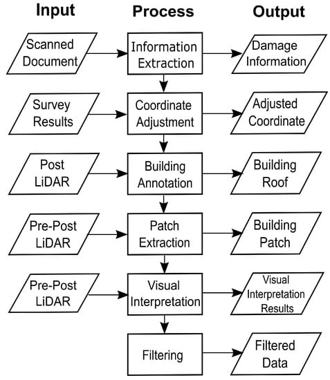
Figure 3.
Dataset creation workflow.
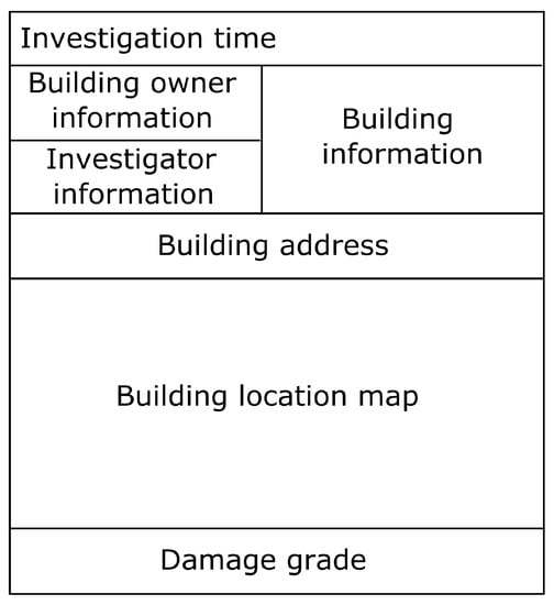
Figure 4.
Simplified recording sheet.
2.2.2. Coordinate Adjustment
The residential buildings in the surveyed areas were densely distributed. The recorded GPS coordinates, therefore, did not always precisely correspond to the correct buildings, due to various factors (e.g., systematic errors or human errors). To eliminate possible erroneous parings of the building and their coordinates, we manually adjusted every GPS coordinate. The building point clouds were converted to 2.5D point clouds and visualized along with building GPS coordinates in QGIS. Then, the GPS coordinates were manually moved to the top of the corresponding buildings. In the case of uncertain pairings, we identified the correct buildings by comparing in situ photographs of the buildings, which were tied with GPS coordinates using IDs, and Google Earth historical images.
2.2.3. Building Roof Annotation
The adjusted coordinates were used to locate the corresponding buildings in post-event LiDAR point clouds. Specifically, for each coordinate, we used it as the center and extracted all points within a 10 m square window (with infinite elevation) out of the whole point clouds to visualize using Python PPTK library. Then, the building part of the point clouds was annotated manually and stored in the NumPy Array format. The boundary ambiguities were resolved by visually assessing backscattered intensities, in situ photos, and Google Earth historical images. Note that the buildings were observed by airborne sensors, and thus, the information of structures below roofs was extremely limited. Furthermore, the debris of “collapsed” buildings were excluded, in order to minimize possible incorrect annotations. In the case of fully “collapsed” buildings, we observed that their roof remained either structurally intact or partially deformed, and thus, their roofs were also annotated. In other words, all of the extracted building data consisted of either structurally damaged roofs in the case of “collapsed” buildings or structurally intact roof for “others” buildings (these roofs may contain surface damage). The reasons for extracting roofs separately are three-fold: The separation of the roofs and surroundings is important for evaluating whether the models are able to classify the input point clouds correctly given only buildings (roofs) themselves. By training DNNs using only building roofs, how the DNNs recognize building damage can be made clearer through visual explanations. The effect of surroundings information could be quantified through comparing the performances of the models using either building roofs or building patches, which include both the buildings and surroundings, for training. For clarity, we call the annotated roofs “building roofs” in this study. The example of building roof is shown in Figure 5.
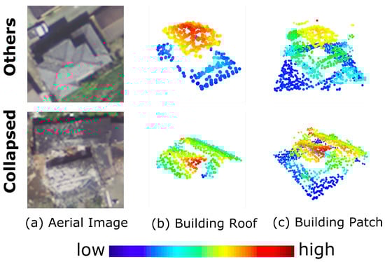
Figure 5.
Examples of annotated buildings. Aerial images were provided by [12]. The point clouds are color-coded by their height values.
2.2.4. Building Patch Extraction
Subsequently, we extracted the building point clouds, along with their surroundings contextual information, which we call the “building patch”. An initial bounding box was computed using the annotated building roof, and subsequently, the longer side of the bounding box was chosen as the size of the square bounding box for patch extraction. Finally, the square bounding box was uniformly dilated with a buffer, in order to increase the amount of surroundings information. In this study, the buffer was set as 2 m. An example of an extracted building patch is shown in Figure 5. After building patch extraction using post-event LiDAR, pre-event building patches were also extracted using the bounding boxes of post-event patches. Note that the buildings in pre-event patches were no longer at the center of the patch, due to coseismic displacement.
2.2.5. Visual Interpretation
It is common practice to use visually interpreted building damage using aerial images as reference data to train the DNNs for emergency mapping [9,10]. Therefore, we visually interpreted the post-event LiDAR dataset, in order to extract “collapsed” buildings, according to the damage pattern chart proposed by [38] (defined as “D5” in [38]), independently of the work of [36], where only “story-collapsed” buildings were extracted by examining the in situ photographs. Note that we only visually interpreted and classified the building point clouds that were initially classified as destroyed (not necessarily collapsed) buildings by field investigations into either the “others” or “collapsed” classes. Subsequently, buildings that were not classified as destroyed buildings by the field investigations were labeled as “others”. For the sake of brevity, we call the visual interpretation results the “V-reference”, while the photographically interpreted “story-collapsed” data [36] are called the “P-reference”. The distributions of two reference data (after filtering, which is explained in the next section) are shown in Table 1.

Table 1.
Class distribution of the reference data used in this study. V, visual; P, photographic.
2.2.6. Filtering
The sizes of the buildings were non-uniformly distributed in the extracted buildings. The areas of some buildings were extremely small, comprised of no more than 100 points (e.g., very small houses), whereas some of them were extremely large (e.g., temples) with more than a few thousand points. In order to reduce such outliers, percentile-based filtering was implemented. We first calculated the areas of each building and the numbers of points it contained. Then, for the calculated areas and number of points, we retained the buildings between the first and 99th percentiles. Note that we only retained the buildings that met both aforementioned conditions. The resulting V-reference and P-reference distributions are shown in Table 1. As shown in Table 1, the distribution of the two classes is imbalanced for both reference data. Consequently, to mitigate the potential adverse effects of the imbalanced distribution, we used a weighted loss function during training, which is a widely accepted practice in imbalanced learning.
2.3. Comparisons of V-Reference and P-Reference
The V-reference vs. P-reference comparison is shown in Table 2. Considering the definition of “collapsed” and “story-collapsed” in which the latter belongs to the former, the overestimation is allowed and underestimation is forbidden. In fact, visual interpretation overestimated 156 buildings as “collapsed”, whereas it underestimated 14 buildings as “others”. The reasons for the overestimations are shown in Table 3. We found that more than half of the buildings were overestimated by visual interpretation because of the roof deformations visible in the post-event LiDAR data. However, some in situ photographs of those buildings captured either partial information or occluded by debris and surrounding objects such as trees, which made it difficult to certainly identify them as “story-collapsed” buildings. We suspect that [36] removed those ambiguous buildings because their final goal was to construct fragility functions [39], which required the correct identification of “story-collapsed” buildings. Furthermore, some thick blue sheet-covered roofs manifested themselves as continuously deformed roofs. On the other hand, seventy buildings were overestimated as “collapsed” by visual interpretation because of their visible roof inclinations. The other reasons for overestimations include unavailable in situ photographs and demolished buildings, which did not exist when the field survey was carried out. Most of the underestimation was due to the unobservable deformations where their slight deformations were barely detectable by human eyes (by observing LiDAR point clouds) according to the Table 4. Moreover, partially collapsed roofs that demonstrated as disjointed collapse were confusing, as part of the roofs were visually intact. Other minor reasons were later collapsed buildings and demolished (but they were not removed when the field surveys were carried out) buildings, where their collapses occurred during the period between LiDAR acquisitions and field surveys. From the view of collapsed building detection, the overestimation of collapsed buildings is more tolerable than underestimation. Therefore, the visual interpretation results were considered acceptable.
Table 2.
Comparison of the two reference datasets.
Table 3.
The reasons for the overestimations.
Table 4.
The reasons for underestimations.
3. Methodologies and Experimental Settings
3.1. Building Damage Detection Framework
In this study, the holistic damage assessment framework is treated as a supervised classification task following the chart illustrated in Figure 6. The selected algorithm receives airborne LiDAR point clouds as input and generates predicted damage grades as output. The predicted damage grades are compared with the reference data, in order to assess the performance. To evaluate the models’ capabilities to detect damages given only 3D geometrical information derived from point clouds, we limited the input features of each point to 3D spatial coordinates. Three types of data availability scenarios were included in the framework. For each scenario, several selected algorithms were applied to predict the damage grades for each building. In the first experiment, the models were trained using the V-reference, in order to assess their abilities to detect “collapsed” buildings. The resulted mapping was called the “emergency mapping”, as such a type of mapping using visually interpreted reference data is needed shortly after a disaster occurs. In the second experiment, the models were trained from scratch using P-reference data for detecting “story-collapsed” buildings specifically. The resulting mapping, which is called the “fine-grained analysis” in this study, aims to extract fine-grained information (i.e., the models extracted “story-collapsed” cases among “collapsed” cases). The “fine-grained analysis” was expected to be more challenging compared to “emergency mapping”. First reason is that the “story-collapsed” buildings belong to the broader category of “collapsed” buildings, and therefore, the smaller intra-class variations between “story-collapsed” buildings and other collapsed buildings might make classification harder. The second reason is that the P-reference was created independently from the input data (point clouds) using photographs, which certainly makes the task difficult compared to using the V-reference, which was directly created using point clouds, as reference data. Such an experiments, however, is meaningful to verify if the point cloud-based DNNs are capable of achieving high performance given the reference data created based on a different data format (e.g., image). The results of two experiments were compared to justify our conjectures.
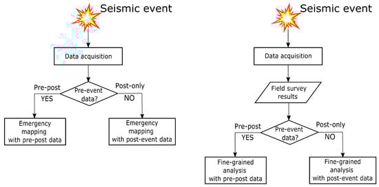
Figure 6.
Overall damage detection framework of emergency mapping (left) and fine-grained analysis (right).
3.1.1. Data Availability
Under ideal circumstances, the joint usage of pre- and post-event LiDAR data should be able to provide the most accurate classification results [3]. Therefore, we carried out damage detection under the pre–post scenario by using both pre- and post-event building patches as training and testing data. In practice, pre–post patches of the same building were fed into the network simultaneously, from which a prediction representing its damage grade considering both pre-event and post-event data was generated. In the case that pre-event data were not readily available, damage assessment using only post-event data was performed. The algorithm received post-building point clouds and predicted their damage grades. Two types of independent post-only scenarios were designed: post-building patch and post-building roof. In the former scenario, a post-building patch, which contains the targeted building, as well as its surroundings (e.g., trees, roads), were used as training and testing data for DNNs. In the latter scenario, post-building roofs were used as training and testing data for DNNs. In all scenarios, the assignment of buildings for training and testing was shared given the same reference data (either V-reference or P-reference). In other words, if the reference data were fixed, each scenario received the same buildings as training and testing data, and they only differed in the number (pre–post is 2, post-only is 1) and format (pre–post patches, post-building patches, or post-building roofs) of the input data. Such experimental settings made direct comparison among scenarios possible. We expected that the pre–post scenario would have the best-achievable performance, while comparisons between post-building patch and roof would reveal the effect of surroundings (e.g., tree, ground) with respect to the final performance.
3.1.2. Algorithms
Several basic, as well as cutting-edge algorithms were chosen to conduct damage assessment experiments. The basic algorithm revealed the baseline performance, whereas the cutting-edge ones (which were direct extensions of the basic ones) were employed to reveal the influence of algorithmic improvements on the final performances. The performances of different algorithmic design choices were also compared, such that the analysis revealed promising directions for further algorithmic developments. The chosen algorithms and their representative features are briefly introduced in the following sections.
PointNet [20], which was chosen as the baseline classifier, is a network that directly takes 3D point cloud as input and makes a prediction based on both independent per-point features, as well as aggregated global features; hence, it is able to grasp both the local geometrical details and the global abstract shape of the point cloud. Its network design ensures there is no information loss due to input conversion. In addition, it has been theoretically and empirically proven to be robust to various 3D point cloud related tasks. Therefore, we chose PointNet as our baseline network.
PointNet++ [21] is a variant of PointNet. It has been shown to achieve hierarchical learning by stacking multiple sampling and grouping layers, as inspired by the extremely successful U-Net [40] architecture. Moreover, it extends PointNet by using a translation-invariant convolutional kernel in each sampling and grouping process, such that the network is aware of metric space interactions among neighboring points. Consequently, PointNet++ considerably improves upon the performance of PointNet, by a large margin, in various tasks.
DGCNN [22] extends PointNet by introducing edge convolution layers, in order to make the network aware of metric space interactions (similarly to PointNet++). The difference between DGCNN and PointNet++ lies in the definition of a neighborhood. PointNet++ builds a spatial (3-dimensional) radius graph for each convolution process, whereas DGCNN adopts feature-level KNN graphs for convolutions. This feature-level KNN enables DGCNN to learn not only spatial patterns, but also feature space patterns. Additionally, PointNet++ achieves hierarchical learning by down-sampling, while DGCNN always maintains the full number of points in every layer.
By extending a single-input network to double inputs, this study proposes a unified framework for adapting any aforementioned networks to the pre–post classification scenario. Inspired by [41], we designed a Siamese-based classification framework. The architecture of this framework is shown in Figure 7. This framework accepts two point clouds—the pre- and post-event point clouds—and transforms them into compact representations through the chosen backbone network. Two compact representations are subsequently aggregated element-wise by an aggregation operation. Finally, the resulting feature is fed into three fully-connected layers to obtain the final classification scores. Note that the backbone networks for each input are weight shared. Therefore, the networks naturally transform similar inputs into similar high-dimensional features. Subtraction, addition, and multiplication are the most commonly used types of element-wise aggregation. In this work, subtraction was adopted because making classification based on pre–post difference conceptually follows change detection, which was proven to be successful in previous works [3].
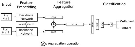
Figure 7.
Proposed framework to extend a single-input network to the double-input pre–post scenario. N represents the number of points in the point clouds. Numbers indicates the dimensions of the features. The framework receives two point clouds and aggregates them to generate a single 1024-dimensional vector. The vector is subsequently fed into fully-connected layers to obtain the final classification scores.
3.1.3. Performance Evaluation
Classification performance was measured using K-fold cross-validation, in order to robustly estimate the prediction accuracy (with the standard deviation). Specifically, the whole dataset was split into K (5, in this study) distinct sets in a stratified manner. In each execution, K−1 sets were regarded as training sets, whereas 1 set was regarded as the test set. Therefore, this process was repeated K times, and the final score was the average of K executions (with the standard deviation). The performance of the classification results are quantitatively reported using the standard accuracy measures (precision and recall). They are reported as the average and standard deviation over the results of the K-fold cross-validation.
3.2. Sensitivity Analysis
The damage grade of a building is determined by various damages, such as deformations, cracks, and inclinations of each structural component (i.e., roofs, walls, and foundations), according to [35]. In order to validate whether trained models can make correct predictions by virtually locating the damaged parts of buildings, a sensitivity analysis was carried out under the post-only scenario. Considering the fact that the roof is the major observable part of a building measured by airborne LiDAR, we expected that our analyses could reveal DNNs’ capability of locating roofs and damages to it.
Verifying Damage Localization by a Visual Explanation
Despite the outstanding performance that DNNs can provide, it is also essential to verify that such performances are gained through proper understanding of the given problem [42]. Methods providing the interpretation of the results of DNNs have, therefore, become critically important for validating their performance. Furthermore, its importance becomes even more magnified in applications such as damage detection, where the reliability of the model should be carefully examined.
Sensitivity analysis is a powerful tool for explaining the decisions made by DNNs [43,44], whereas some recent works [45,46] have tried to provide a visual explanation by highlighting the particular region of the input image that model depended on for classifying this input image. Although their approaches can provide meaningful representations of how these models make decisions, the types of architectures are limited to 2D image-based DNNs. A point cloud saliency map [47] has recently been proposed, in order to evaluate the per-point importance. Nevertheless, this approach is difficult to adapt to complex outdoor scenes, such as destroyed buildings with surrounding objects.
As such, we propose a simple visualization method to qualitatively assess how the models recognize damages. Concretely, the method—which we call Iterative Partial Set Importance (IPSI)—calculates the importance score of each point, with respect to classification performance. We assume that the output probability of the correct class decreases if an important part of the point cloud is removed and that the reduction of probability is correlated to the degree of importance of the removed part. Let be an input point cloud. The spherical neighborhood of a point in is defined as:
where r is a pre-defined radius. The value of r (0.2, in this study) was chosen as the smallest searching radius used in set abstractions of PointNet++. The value of r should not be too large because the importance score would be too high for each point if a large number of points are removed in each IPSI iteration. Radius search was chosen over KNN because the former can always provide searched points in a constant volume while the volume of the searched points from the latter depends on the point density. We further defined the output probability of a correct class by a network given an input set as . The baseline importance score was set to . Then, we calculated the score of the set , which is , and set it as the current score. Inspired by [48], we defined the importance score of as the difference between the baseline score and the current score . When this score is positive, the importance of the removed part is directly indicated. On the other hand, it is beneficial to remove the part when the score is negative. The IPSI procedure is shown in Algorithm 1 below.
| Algorithm 1 IPSI. |
|
3.3. Ablation Study
In the case of early-stage damage mapping, it is important to know the minimal number of samples required, with respect to the achievable performance. Therefore, we gradually reduced the number of training samples and measured the corresponding final performance without changing the test data. The reduction rate (and numbers of buildings reduced) of training data was set to 0% (4829), 50% (2414), 90% (482), 95% (241), and 99% (48), respectively. Each reduction used a stratified sampling process, where the initial distribution ratio between classes was preserved. The algorithms used in the ablation study were the ones that performed the best under each data availability condition (pre–post, post-building patch, and post-building roof) considering the mean recall of two classes. The reference data used were the V-reference, as visual interpretation data are often used in emergency mapping.
3.4. Generalization Test
To evaluate the generalization ability of the trained model to detect collapsed buildings, the damage assessment using LiDAR data acquired through a different sensor in a geographical region having a different major architectural style was implemented. The overview of the test site is shown in Figure 8. The test site was Port-au-Prince, Haiti, which was struck by an earthquake in 2010. Approximately 316,000 people were killed and 97,294 buildings destroyed [49]. The vast majority of buildings were the reinforced concrete type, which strongly differed from the major building types in the Kumamoto region. The data were obtained between 21 January and 27 January 2010, with an average density of 3.4 points/m2 [50].
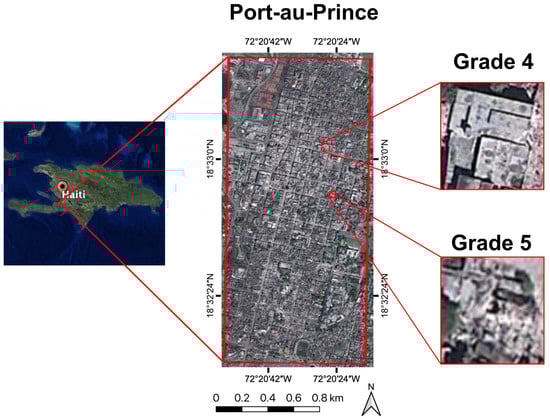
Figure 8.
Location of the acquired dataset used for the generalization test.
Training and testing data were prepared using visually interpreted building footprints provided by a third party. The building patches were extracted following the creation process of the Kumamoto dataset. The damage grades of buildings were estimated according to the EMS-98 scale [51]. Grade 4 (G4) and Grade 5 (G5) buildings were used for the generalization tests. G4 buildings are the buildings with partial deformations, but the majority of their structure remain intact, whereas G5 buildings are totally collapsed buildings according to [38]. G4 buildings were assigned to the “others” class, while G5 buildings were assigned to the “collapsed” class during the experiments. The number of buildings is shown in Table 5. Half of the data were used as training and the other half for testing. The inter-class ratio was preserved using stratified random sampling. A series of experiments was implemented to quantitatively assess the generalization ability of the pre-trained model (i.e., trained using developed Kumamoto post-building patch dataset). Note that all the post-building patches in the Kumamoto dataset were used for training. The training sample rates for the pre-trained model were controlled and gradually increased from 0% to 100%. Additionally, a model was trained from scratch only using the Haiti data, in order to verify the usefulness of pre-training.
Table 5.
Number of buildings in the Haiti dataset. G, Group.
3.5. Implementation Details
All of the models were implemented using PyTorch [52]. We adopted Adam [53] as our choice for the optimizer. The initial learning rate for the models was 0.007, which was scaled down by 0.7 every 25 training epochs. The total number of epochs was 250 for all runs. We used two NVIDIA Tesla P100 GPUs, provided by TSUBAME3.0 supercomputer, for both training and testing. The batch size was set to 16 per GPU during training. The number of points in an input point cloud was set to 1024 to achieve batch training. The batch size was set to 1 during testing, in order to predict the point cloud with different point numbers. Random rotation around the z (or vertical) axis was applied on the fly during training for data augmentation purposes. Furthermore, the input data were scaled into the unit ball, meaning that the lengths of edges from the centroid of a building instance to any point in it were normalized to the 0–1 range by dividing each edge by the longest edge. Weighted cross-entropy [54] was used for the loss function for all experiments, in order to deal with class imbalances where the sample size of “others” was considerably larger than “collapsed”. The weight of each class is calculated as:
where c is a class, is the total number of samples that belong to class c in the training data, and N is the total number of training samples. For PointNet++, the number of sampled points in 3 subsequent set abstractions was set to 512, 128, and 32, while the searching radii for each set abstraction were 0.2, 0.4, and 0.8, respectively. The parameter K, which is the number of neighbors in the EdgeConv process, used in DGCNN was set to 20 following the original paper [22].
4. Results
In this section, the results of our experiments are presented. The results of two damage detection experiments with distinct purposes are quantitatively analyzed. Subsequently, the results of the sensitivity analyses are shown by visualizing the typical recognition pattern of the trained model using IPSI. The typical misclassification types are introduced using IPSI as well. Then, the results of the ablation study showing the robustness of the models considering sample reduction are presented, followed by the results of the generalization tests. Finally, this section concludes with a discussion regarding our significant findings and the challenges derived from the experiments.
4.1. Results of Emergency Mapping
The experimental results of early-stage mapping are shown in Table 6. As expected, the highest performance was achieved when pre- and post-event data were both available, followed by the building patch and the building roof. The predictions became more stable, in terms of standard deviations, when more information was available. In addition, the pre–post approach also achieved the best performance in every category and performance metric. Therefore, it is clear that the pre–post approach is the most ideal condition for 3D point cloud-based deep learning for damage detection. Furthermore, our proposed general extension framework was proven to be effective, achieving high performance with all chosen modern backbone networks. However, extended PointNet achieved the highest score, compared to other advanced architectures. Presumably, the reason for this is that the introduction of the translation-invariant convolutional kernel made it harder for the networks to capture abstract global changes, such as global translation and deformation. Further exploitation of this topic is out of the scope of this study, and hence, we leave it to future work.
Table 6.
Emergency mapping results. The best performances of each category and data availability are highlighted.
To our surprise, the best-performing network using the post-event building patch was only inferior to the best performing pre–post one by a small margin (0.01). In other words, modern deep neural networks using this point cloud data can perform almost as well as the pre–post one without pre-event data. The PointNet++ architecture demonstrated remarkable performance, surpassing all other networks using building patches by a large margin. Furthermore, it even demonstrated better performance than the pre–post extended PointNet++ and DGCNN.
The overall performance was drastically reduced when the input data were roof only. This situation was consistent except for the recall value of “others” and the precision value of “collapsed” of DGCNN. Therefore, the reduction of contextual information almost surely decreases the classification performance. The largest gap of recall was presented in the “collapsed” class of DGCNN. It was also obvious that removing contextual information made the results more widely varied, as demonstrated by increasing standard deviations among K runs. Such a phenomenon indicated that the predictions of some samples can become stable under the presence of contextual information, showing a possible large dependence on the surrounding environmental elements.
4.2. Results of Fine-Grained Analysis
The results of fine-grained analysis closely resembled the pattern of emergency mapping according to Table 7, with slightly reduced performance. The reduction of performance may due to the ambiguities between “story-collapsed” and “collapsed”, for which the latter contains the former according to the definition of G5 in the damage pattern chart [38]. In general, the best-performing models under each achieved high recalls under each data availability scenario, indicating that the models were able to accurately detect story-collapsed buildings among all buildings. In addition, the results proved that the point cloud-based DNNs can perform well given reference data created using in situ photographs.
Table 7.
Results of fine-grained analysis. The best performances in each category and data availability are highlighted.
4.3. Results of Sensitivity Analysis
In this section, the results of sensitivity analysis are presented. The models used were PointNet++ trained by using either post-building roof or post-building patch as training data. The damage localization results are shown to verify whether the model can make correct predictions by focusing on damaged parts. In addition, the failure cases were also analyzed to reveal the limitations of modern DNNs.
4.3.1. Damage Localization
One of the most obvious indicators of damage to a building is deformations. The top row of Figure 9b clearly shows that the model could localize the partial deformation occurring in the roofs of buildings, where other parts of the roofs were relatively intact in the captured point clouds. As shown in Figure 9c (i.e., of the same row), the highlighted part was extremely important for classifying this point cloud, as the result became incorrect when these points were removed. When the input was the building patch, the model prioritized the debris instead of other deformed parts of the roof, according to Figure 9d. However, the model tended to localize many parts of the building, but the maximum assigned score remained low (0.13) when the input was a completely collapsed building with a heavily damaged roof. Therefore, the classification results of such buildings were stable. The building in the bottom row was story-collapsed with little roof damage and a minor inclination. Although it was correctly classified, the base score of the building was lower (0.67) compared to those in the upper rows (0.94+). The low base score indicated that the classification result was unstable and could possibly be easily misclassified by removing some parts of it, as is shown in the bottom row of Figure 9c.
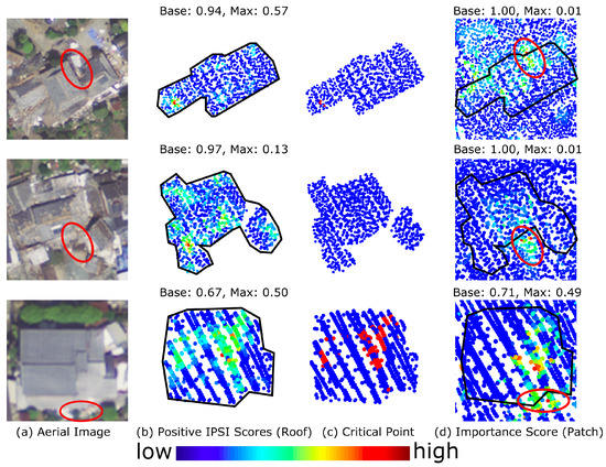
Figure 9.
Results of sensitivity analysis: The low-to-high scale bar shows the positive Iterative Partial Set Importance (IPSI) score within each building instance. The baseline probability and maximum importance values are shown in (a) and (d). (a) shows the aerial images [12]; (b) shows the positive IPSI scores (roof); (c) shows “critical points” that change the classification results if they are removed; and (d) shows the positive IPSI scores (patch).
4.3.2. Failure Cases
The typical misclassification patterns using building roofs as input are shown in Figure 10. The negative IPSI scores for misclassified buildings in Figure 10 indicate that the probability of correct class increases when removing the corresponding part. In other words, the highlighted points show the possible causes of misclassifications. For the “others” class, as illustrated in the top row, additional structures were one of the misclassification sources. They tended to make the roofs discontinuous, thus making them more similar to damaged roofs. The second row shows that the model located the deformations correctly, but overemphasized it, which led to the misclassification. In terms of the “collapsed” class, the first cause of misclassification was that the model was clearly insensitive to the inclination of the roof, indicating that the model made decisions mainly based on the local roughness of the surface, rather than its global characteristics. It was highly challenging for the model to capture slight but global deformations of the buildings; for instance, the model failed to detect the collapsed building in the bottom row, for which the ridge was non-horizontal without obvious deformation to the roof.
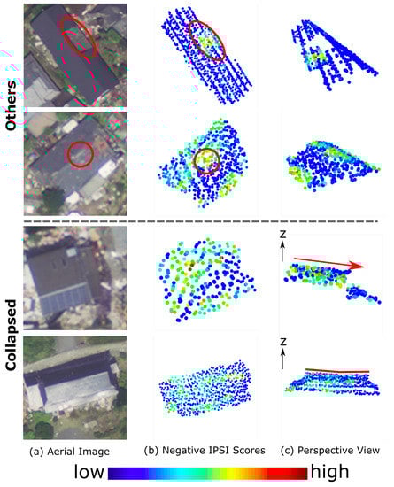
Figure 10.
Examples of misclassifications when using building roofs. Buildings in the first two rows belong to the “others” class, but were misclassified as “collapsed”, whereas buildings in the last two rows belong to “collapsed”, but were misclassified as “others”. (a) shows the aerial image [12]; (b) shows negative IPSI scores (roof); and (c) shows the perspective views, from which the causes of misclassification can be clearly observed.
Even though the addition of contextual information did improve the overall performance, it also induced more types of errors. In the top row of Figure 11, the model showed the largest importance score at the slope with a small amount of debris or soil near the captured building. The reason for this is that irregularly distributed debris is often found in the vicinity of collapsed buildings. Tall trees and low bushes corresponded to high scores in the second row. As vegetation presented itself as irregularly scattered points in the LiDAR scan resembling debris, it also confused the model and led to misclassification. On the other hand, the model, again, failed to capture large inclinations given more contextual information, as indicated by Figure 11c. Similar to the case of Figure 10c, the model still failed to capture minor but global deformations, as shown in Figure 11c.
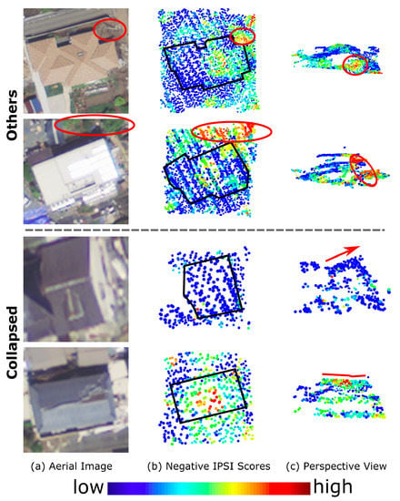
Figure 11.
Examples of misclassifications using building patches. Buildings in the first two rows belong to the “others” class, but were misclassified as “collapsed”, whereas buildings in the last two rows belong to “collapsed”, but were misclassified as “others”. (a) shows aerial images [12]; (b) shows negative IPSI scores (patch); black lines depict the boundaries of building roofs; and (c) shows the perspective views, from which the causes misclassification can be clearly observed.
4.4. Results of the Ablation Study
The results of the ablation study are shown in Figure 12. As expected, the performance using pre–post data was extremely robust to data reduction, achieving approximately 0.85 of mean recall with only 1% (48) of the training samples. This suggests that our proposed framework is effective for damage detection when both pre- and post-data are available. On the other hand, the performance and stability of both roof and patch decreased with increasing reduction rates. However, their performances were still acceptable (around 0.83) after removing 90% of the training data. The scores of the building roofs became higher than those of the building patches after a 10% reduction. Nonetheless, the scores of the roof were closely followed by those of the building patches, until they reached a reduction rate of 1%.
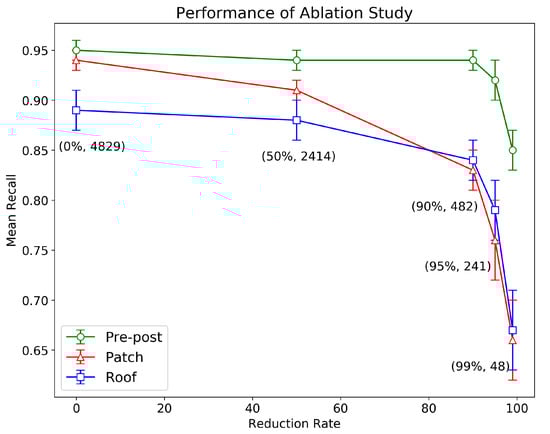
Figure 12.
Performance of the ablation study.
4.5. Results of the Generalization Test
The results of the generalization tests are shown below in Table 8. The pre-trained model achieved acceptable performance, even without any training data. This indicates that the trained model was capable of learning common features across different architectural styles. The performance on the “collapsed” class was higher than that with “others”. This was expected, as the degree of similarity between G5 of masonry buildings and wooden buildings is higher than that of G4 buildings. The model achieved the highest mean recall when 50% of the training data were used. However, it only outperformed the non-trained model by a small margin (0.03), demonstrating the promising universality of the model. Surprisingly, the pre-trained model with 100% of the data scored lower than that using 50% of the data. Although this case is worthy of further investigation, in this work, we focused on the best-achievable performance under given conditions, rather than explaining the complex behavior of transfer learning. Furthermore, the usefulness of pre-training can be clearly seen, as the non-trained model with pre-training outperformed the fully-trained model (100%) without pre-training.
Table 8.
Results of the generalization experiments. The best performances among each category are highlighted.
5. Discussion
5.1. Potential of LiDAR for Building Damage Detection
Our series of experiments and analyses fully demonstrated the high potential of the proposed LiDAR dataset for building damage detection approaches, in terms of overall performance and damage recognition patterns. In view of its operational advantages, a LiDAR sensor can operate under most weather conditions using the active sensing principle. Furthermore, collapsed building detection is of highest importance, as it may greatly endanger residents, compared to other types of damage. Such buildings that are hardly visible or remain highly uncertain from vertical images can be clearly observed using airborne LiDAR 3D point clouds. Therefore, the visual interpretation and automatic detection of collapsed buildings using LiDAR is generally preferred, compared to aerial image-based methods. Moreover, the generalization test results also confirmed that using point cloud data can lead to acceptable performances without additional training data, even if the buildings in the dataset have very different architectural styles, compared those in the dataset for pre-training.
However, the current limitation of LiDAR, compared to aerial imagery, is also apparent. First of all, the operational cost and priority of LiDAR are still behind the aerial images, which may be resolved through the recently increasing interest in hardware development and rapid advancement of LiDAR technology in the scientific and industrial fields. In terms of the expected performance, aerial images are clearly advantageous for detecting lower damages, due to their rich radiometric and textural information. Consequently, the wisest decision to make is to combine these complementary technologies for the highest performance [19,55]. However, the fusion of two distinct data types is not trivial, and thus, it is left as future work.
5.2. Effectiveness and Challenges of the Proposed Visual Explanation Method
IPSI intuitively illustrated the decisions of models relating to particular building damages. Visualization using IPSI showed that the model was able to precisely locate partial damages on roofs by assigning high importance scores to nearby points when the other parts were less damaged. On the other hand, the models succeeded to detect multiple deformations by assigning low scores to them if the roofs were uniformly damaged. By adding contextual information to building roofs, the models were trained to detect debris effectively, similarly to human operators.
More importantly, IPSI revealed the challenges that modern point cloud-based DNNs face, considering building damage detection. The most prominent misclassification was that the models failed to detect global damages, such as inclination and slight global deformations. These types of damage cannot be detected by merely locally assessing the surface, which modern DNNs are good at. In addition, they tended to consider roofs to be continuous which led to misclassification of intact roofs having additional structures. Secondly, the addition of contextual information obviously caused the models to depend too much on context, leading to the diffusion of the focus region away from the buildings. Therefore, the reliability of the models was reduced, as the models did not explicitly localize the buildings.
Despite its effectiveness and simplicity, IPSI has some challenges that need to be addressed. The efficient implementation of IPSI is necessary, as it iterates over all points in the given set. Therefore, the computational cost surges with an increase in the number of points or density. This could be mitigated by introducing sampling methods that uniformly preserve 3D geometries [21] or parallelizing the algorithm across a large number of CPUs. Additionally, the definition of importance can be improved by incorporating gradient information [45], which shows explicit relationships with classification scores.
5.3. Future Study
With the aim of improving building damage detection method performances, we intend to develop a model that is inclination-sensitive. Data fusion of aerial images and LiDAR point clouds will also be investigated, for joint exploitation of individual advantages. In terms of improving reliability, one possible direction of development is to use regularization, such that the model is aware of buildings when building patches are used. Moreover, the further improvement of visual explanation methods should also be taken into consideration, in order to validate the reliability of model decisions.
6. Conclusions
In this paper, we focus on developing a large-scale dataset, which is tailored to building damage detection using 3D point cloud data. Three forms of output are created for evaluating different data availability scenarios: pre–post building patches, post-building patches, and post-building roofs. The building roofs are separated from patches, such that the recognition of buildings could be independently assessed without interference by contextual information. Several damage assessment experiments using the developed dataset are implemented, using both basic and modern 3D deep learning algorithms under varying data availability scenarios. A general framework extending single-input to multiple-inputs is proposed, in order to adapt single-input networks to the pre–post classification scenario. The results show that the best-performing networks under each data availability scenario are able to achieve satisfactory emergency mapping results. In addition, the experimental results regarding the extraction of fine-grained damage type (story-collapsed, in this study) show that the trained models are able to achieve comparable accuracy to emergency mapping procedures.
A visual explanation method is proposed to qualitatively assess the per-point importance, with respect to the classification performance. Through visualization, we confirm that the trained models are capable of locating deformations occurring on roofs, as well as the debris scattered around buildings. It also reveals that the models tend to overemphasize the local deformation, as well as debris-like objects (e.g., bushes and piles of soil), leading to misclassifications. Meanwhile, visualization of the results shows that the cutting-edge models lack the ability to detect inclinations and slight global deformations.
Finally, we conduct an ablation study and a generalization test. By reducing the number of samples, the ablation study reveals that the proposed pre–post framework is extremely robust to data reduction. Though not comparable to the pre–post approach, the post-building patches and roofs are also able to achieve acceptable performance with only 10% of the training data. The generalization ability of the model is also tested, using LiDAR data acquired using a distinct sensor with buildings having different architectural styles compared to those in the dataset used for pre-training. The model trained using the developed dataset achieves moderate performance without training data, demonstrating the promising application of point clouds in transfer learning.
Future study will include the development of an inclination-sensitive model, data fusion with aerial images, and improvement of the proposed visual explanation model by adding gradient information.
Author Contributions
Conceptualization, H.X.; data curation, H.X.; formal analysis, H.X.; funding acquisition, M.M.; methodology, H.X.; project administration, H.X.; resources, M.M., M.I., K.K., and K.H.; software, H.X.; supervision, M.M.; validation, H.X.; visualization, H.X.; writing, original draft, H.X.; writing, review and editing, H.X., T.S., and M.M. All authors read and agreed to the published version of the manuscript.
Funding
This research was supported in a part by “the Tokyo Metropolitan Resilience Project” of the Ministry of Education, Culture, Sports, Science and Technology (MEXT) of the Japanese Government and the National Research Institute for Earth Science and Disaster Resilience (NIED).
Acknowledgments
This work is based on data services provided by the OpenTopography Facility with support from the National Science Foundation under NSF Award Numbers 1833703, 1833643, and 1833632. The vector format data used for generating the map are available from the Geospatial Information Authority (GSI) of Japan. The satellite images used to verify the boundary ambiguities in dataset creation were obtained from Google Earth. The satellite image of the test site in the generalization test was also obtained from Google Earth. The building footprints of the Haiti Earthquake were provided by the United Nations Institute for Training and Research (UNOSAT). This study was carried out using the TSUBAME3.0 supercomputer at Tokyo Institute of Technology.
Conflicts of Interest
The authors declare no conflict of interest. The funding sponsors had no role in the design of the study; in the collection, analyses, or interpretation of data; in the writing of the manuscript; nor in the decision to publish the results.
References
- Dell’Acqua, F.; Bignami, C.; Chini, M.; Lisini, G.; Polli, D.A.; Stramondo, S. Earthquake damages rapid mapping by satellite remote sensing data: L’Aquila april 6th, 2009 event. IEEE J. Sel. Top. Appl. Earth Obs. Remote. Sens. 2011, 4, 935–943. [Google Scholar] [CrossRef]
- Matsuoka, M.; Yamazaki, F. Use of satellite SAR intensity imagery for detecting building areas damaged due to earthquakes. Earthq. Spectra 2004, 20, 975–994. [Google Scholar] [CrossRef]
- Dong, L.; Shan, J. A comprehensive review of earthquake-induced building damage detection with remote sensing techniques. Isprs J. Photogramm. Remote. Sens. 2013, 84, 85–99. [Google Scholar] [CrossRef]
- Wieland, M.; Liu, W.; Yamazaki, F. Learning change from Synthetic Aperture Radar images: Performance evaluation of a Support Vector Machine to detect earthquake and tsunami-induced changes. Remote Sens. 2016, 8, 792. [Google Scholar] [CrossRef]
- Bai, Y.; Adriano, B.; Mas, E.; Gokon, H.; Koshimura, S. Object-based building damage assessment methodology using only post event ALOS-2/PALSAR-2 dual polarimetric SAR intensity images. J. Disaster Res. 2017, 12, 259–271. [Google Scholar] [CrossRef]
- LeCun, Y.; Bengio, Y.; Hinton, G. Deep learning. Nature 2015, 521, 436–444. [Google Scholar] [CrossRef] [PubMed]
- Krizhevsky, A.; Sutskever, I.; Hinton, G.E. Imagenet classification with deep convolutional neural networks. In Advances in Neural Information Processing Systems; Curran Associates Inc.: Lake Tahoe, NV, USA, 2012; pp. 1097–1105. [Google Scholar]
- Ci, T.; Liu, Z.; Wang, Y. Assessment of the Degree of Building Damage Caused by Disaster Using Convolutional Neural Networks in Combination with Ordinal Regression. Remote Sens. 2019, 11, 2858. [Google Scholar] [CrossRef]
- Naito, S.; Tomozawa, H.; Mori, Y.; Nagata, T.; Monma, N.; Nakamura, H.; Fujiwara, H.; Shoji, G. Building-damage detection method based on machine learning utilizing aerial photographs of the Kumamoto earthquake. Earthq. Spectra 2020, 36, 1166–1187. [Google Scholar] [CrossRef]
- Miura, H.; Aridome, T.; Matsuoka, M. Deep Learning-Based Identification of Collapsed, Non-Collapsed and Blue Tarp-Covered Buildings from Post-Disaster Aerial Images. Remote. Sens. 2020, 12, 1924. [Google Scholar] [CrossRef]
- Ushiyama, M.; Yokomaku, S.; Sugimura, K. Characteristics of victims of the 2016 Kumamoto Earthquake. Jsnds Jpn. Soc. Nat. Disaster Sci. 2016, 35, 203–215. [Google Scholar]
- Cheng, M.L.; Satoh, T.; Matsuoka, M. Region-Based Co-Seismic Ground Displacement Dectection Using Optical Aerial Imagery. In Proceedings of the IGARSS 2018-2018 IEEE International Geoscience and Remote Sensing Symposium, Valencia, Spain, 22–27 July 2018; pp. 2940–2943. [Google Scholar]
- Moya, L.; Yamazaki, F.; Liu, W.; Yamada, M. Detection of collapsed buildings from lidar data due to the 2016 Kumamoto earthquake in Japan. Nat. Hazards Earth Syst. Sci. 2018, 18, 65. [Google Scholar] [CrossRef]
- He, M.; Zhu, Q.; Du, Z.; Hu, H.; Ding, Y.; Chen, M. A 3D shape descriptor based on contour clusters for damaged roof detection using airborne LiDAR point clouds. Remote Sens. 2016, 8, 189. [Google Scholar] [CrossRef]
- Rehor, M.; Bähr, H.P. Segmention of Damaged Buildings from Laser Scanning Data. Int. Arch. Photogramm. Remote Sens. Spat. Inf. Sci. Bonn Ger. XXXVI Part 2006, 3, 67–72. [Google Scholar]
- Rehor, M.; Bähr, H.P.; Tarsha-Kurdi, F.; Landes, T.; Grussenmeyer, P. Contribution of two plane detection algorithms to recognition of intact and damaged buildings in lidar data. Photogramm. Rec. 2008, 23, 441–456. [Google Scholar] [CrossRef]
- Yonglin, S.; Lixin, W.; Zhi, W. Identification of inclined buildings from aerial lidar data for disaster management. In Proceedings of the 2010 18th International Conference on Geoinformatics, Beijing, China, 12–20 June 2010; pp. 1–5. [Google Scholar]
- Gerke, M.; Kerle, N. Graph matching in 3D space for structural seismic damage assessment. In Proceedings of the 2011 IEEE International Conference on Computer Vision Workshops (ICCV Workshops), Barcelona, Spain, 6–13 November 2011; pp. 204–211. [Google Scholar]
- Vetrivel, A.; Gerke, M.; Kerle, N.; Vosselman, G. Identification of damage in buildings based on gaps in 3D point clouds from very high resolution oblique airborne images. Isprs J. Photogramm. Remote Sens. 2015, 105, 61–78. [Google Scholar] [CrossRef]
- Qi, C.R.; Su, H.; Mo, K.; Guibas, L.J. Pointnet: Deep learning on point sets for 3d classification and segmentation. In Proceedings of the IEEE Conference on Computer Vision and Pattern Recognition, Honolulu, HI, USA, 21–26 July 2017; pp. 652–660. [Google Scholar]
- Qi, C.R.; Yi, L.; Su, H.; Guibas, L.J. Pointnet++: Deep hierarchical feature learning on point sets in a metric space. In Advances in Neural Information Processing Systems; Curran Associates, Inc: Long Beach, CA, USA, 2017; pp. 5099–5108. [Google Scholar]
- Wang, Y.; Sun, Y.; Liu, Z.; Sarma, S.E.; Bronstein, M.M.; Solomon, J.M. Dynamic graph cnn for learning on point clouds. Acm Trans. Graph. 2019, 38, 1–12. [Google Scholar] [CrossRef]
- Liu, Y.; Fan, B.; Xiang, S.; Pan, C. Relation-shape convolutional neural network for point cloud analysis. In Proceedings of the IEEE Conference on Computer Vision and Pattern Recognition, Long Beach, CA, USA, 16–20 June 2019; pp. 8895–8904. [Google Scholar]
- Maturana, D.; Scherer, S. Voxnet: A 3d convolutional neural network for real-time object recognition. In Proceedings of the 2015 IEEE/RSJ International Conference on Intelligent Robots and Systems (IROS), New York, NY, USA, 28 September–2 October 2015; pp. 922–928. [Google Scholar]
- Su, H.; Maji, S.; Kalogerakis, E.; Learned-Miller, E. Multi-view convolutional neural networks for 3d shape recognition. In Proceedings of the IEEE International Conference on Computer Vision, Boston, MA, USA, 7–12 June 2015; pp. 945–953. [Google Scholar]
- Bello, S.A.; Yu, S.; Wang, C.; Adam, J.M.; Li, J. Review: Deep Learning on 3D Point Clouds. Remote Sens. 2020, 12, 1729. [Google Scholar] [CrossRef]
- Liao, Y.; Mohammadi, E.M.; Wood, L.R. Deep Learning Classification of 2D Orthomosaic Images and 3D Point Clouds for Post-Event Structural Damage Assessment. Drones 2020, 4, 24. [Google Scholar] [CrossRef]
- Deng, J.; Dong, W.; Socher, R.; Li, L.J.; Li, K.; Fei-Fei, L. Imagenet: A large-scale hierarchical image database. In Proceedings of the 2009 IEEE Conference on Computer Vision and Pattern Recognition, New York, NY, USA, 20–25 June 2009; pp. 248–255. [Google Scholar]
- Gupta, R.; Goodman, B.; Patel, N.; Hosfelt, R.; Sajeev, S.; Heim, E.; Doshi, J.; Lucas, K.; Choset, H.; Gaston, M. Creating xBD: A dataset for assessing building damage from satellite imagery. In Proceedings of the IEEE Conference on Computer Vision and Pattern Recognition Workshops, Long Beach, CA, USA, 16–20 June 2019; pp. 10–17. [Google Scholar]
- Geiger, A.; Lenz, P.; Urtasun, R. Are we ready for autonomous driving? The kitti vision benchmark suite. In Proceedings of the 2012 IEEE Conference on Computer Vision and Pattern Recognition, Providence, RI, USA, 16–21 June 2012; pp. 3354–3361. [Google Scholar]
- Hackel, T.; Savinov, N.; Ladicky, L.; Wegner, J.D.; Schindler, K.; Pollefeys, M. Semantic3d. net: A new large-scale point cloud classification benchmark. arXiv 2017, arXiv:1704.03847. [Google Scholar]
- QGIS Development Team. QGIS Geographic Information System. Open Source Geospatial Foundation Project. Available online: http://qgis.osgeo.org (accessed on 30 November 2020).
- Chiba, T. Pre-Kumamoto Earthquake (16 April 2016) Rupture Lidar Scan; Distributed by OpenTopography; Air Asia Survey Co., Ltd.: Chiba, Japan, 2016; Available online: https://portal.opentopography.org/datasetMetadata?otCollectionID=OT.052018.2444.2 (accessed on 5 November 2020).
- Chiba, T. Post-Kumamoto Earthquake (16 April 2016) Rupture Lidar Scan; Distributed by OpenTopography; Air Asia Survey Co., Ltd.: Chiba, Japan, 2016; Available online: https://portal.opentopography.org/datasetMetadata?otCollectionID=OT.052018.2444.1 (accessed on 5 November 2020).
- Cabinet Office of Japan (2018): Operational Guideline for Damage Assessment of Residential Buildings in Disasters. Available online: http://www.bousai.go.jp/taisaku/pdf/h3003shishin_all.pdf (accessed on 21 October 2020).
- Kawabe, K.; Horie, K.; Inoguchi, M.; Matsuoka, M.; Torisawa, K.; Liu, W.; Yamazaki, F. Extraction of story-collapsed buildings by the 2016 Kumamoto Earthquakes using deep learning. In Proceedings of the 17th World Conference on Earthquake Engineering, Sendai, Japan, 13–18 September 2020. [Google Scholar]
- Cabinet Office of Japan (2020): Website of Disaster Prevention. Available online: http://www.bousai.go.jp/taisaku/unyou.html (accessed on 2 December 2020).
- Okada, S.; Takai, N. Classifications of structural types and damage patterns of buildings for earthquake field investigation. In Proceedings of the 12th World Conference on Earthquake Engineering (Paper 0705), Auckland, New Zealand, 30 January–4 February 2000. [Google Scholar]
- Matsuoka, M.; Nojima, N. Building damage estimation by integration of seismic intensity information and satellite L-band SAR imagery. Remote Sens. 2010, 2, 2111–2126. [Google Scholar] [CrossRef]
- Ronneberger, O.; Fischer, P.; Brox, T. U-net: Convolutional networks for biomedical image segmentation. In Proceedings of the International Conference on Medical Image Computing and Computer-Assisted Intervention, Munich, Germany, 5–9 October 2015; Springer: Cham, Switzerland, 2015; pp. 234–241. [Google Scholar]
- Koch, G.; Zemel, R.; Salakhutdinov, R. Siamese neural networks for one-shot image recognition. In ICML Deep Learning Workshop; JMLR.org: Lille, France, 2015; Volume 2. [Google Scholar]
- Montavon, G.; Samek, W.; Müller, K.R. Methods for interpreting and understanding deep neural networks. Digit. Signal Process. 2018, 73, 1–15. [Google Scholar] [CrossRef]
- Zurada, J.M.; Malinowski, A.; Cloete, I. Sensitivity analysis for minimization of input data dimension for feedforward neural network. Proceedings of IEEE International Symposium on Circuits and Systems-ISCAS’94, London, UK, 30 May–2 June 1994; IEEE: New York, NY, USA, 1994; Volume 6, pp. 447–450. [Google Scholar]
- Zeiler, M.D.; Fergus, R. Visualizing and understanding convolutional networks. In Proceedings of the European Conference on Computer Vision, Zurich, Switzerland, 6–12 September 2014; Springer: Cham, Switzerland, 2014; pp. 818–833. [Google Scholar]
- Selvaraju, R.R.; Cogswell, M.; Das, A.; Vedantam, R.; Parikh, D.; Batra, D. Grad-cam: Visual explanations from deep networks via gradient-based localization. In Proceedings of the IEEE International Conference on Computer Vision, Venice, Italy, 22–29 October 2017; pp. 618–626. [Google Scholar]
- Chattopadhay, A.; Sarkar, A.; Howlader, P.; Balasubramanian, V.N. Grad-cam++: Generalized gradient-based visual explanations for deep convolutional networks. In Proceedings of the 2018 IEEE Winter Conference on Applications of Computer Vision (WACV), Lake Tahoe, NV, USA, 12–15 March 2018; IEEE: New York, NY, USA, 2018; pp. 839–847. [Google Scholar]
- Zheng, T.; Chen, C.; Yuan, J.; Li, B.; Ren, K. Pointcloud saliency maps. In Proceedings of the IEEE International Conference on Computer Vision, Seoul, Korea, 27–28 October 2019; pp. 1598–1606. [Google Scholar]
- Breiman, L. Random forests. Mach. Learn. 2001, 45, 5–32. [Google Scholar] [CrossRef]
- M7.0—Haiti Region. Available online: http://earthquake.usgs.gov/earthquakes/eventpage/usp000h60h#general_summary (accessed on 21 October 2020).
- World Bank—Imagecat Inc. Rit Haiti Earthquake LiDAR Dataset. Available online: http://opentopo.sdsc.edu.gridsphere/gridsphere?cid=geonlidarframeportlet&gs_action=lidarDataset&opentopoID=OTLAS.072010.32618.1 (accessed on 21 October 2020).
- Grünthal, G. European Macroseismic Scale 1998; Technical Report; European Seismological Commission (ESC): Tel Aviv, Israel, 1998. [Google Scholar]
- Paszke, A.; Gross, S.; Massa, F.; Lerer, A.; Bradbury, J.; Chanan, G.; Killeen, T.; Lin, Z.; Gimelshein, N.; Antiga, L.; et al. PyTorch: An Imperative Style, High-Performance Deep Learning Library. In Advances in Neural Information Processing Systems 32; Wallach, H., Larochelle, H., Beygelzimer, A., d’Alché-Buc, F., Fox, E., Garnett, R., Eds.; Curran Associates, Inc.: Vancouver, BC, Canada, 2019; pp. 8024–8035. [Google Scholar]
- Kingma, D.P.; Ba, J. Adam: A method for stochastic optimization. arXiv 2014, arXiv:1412.6980. [Google Scholar]
- Lao, Y. Open3D-PointNet2-Semantic3D. Available online: https://github.com/intel-isl/Open3D-PointNet2-Semantic3D (accessed on 1 December 2020).
- Qi, C.R.; Chen, X.; Litany, O.; Guibas, L.J. Imvotenet: Boosting 3d object detection in point clouds with image votes. In Proceedings of the IEEE/CVF Conference on Computer Vision and Pattern Recognition, Seattle, WA, USA, 14–19 June 2020; pp. 4404–4413. [Google Scholar]
Publisher’s Note: MDPI stays neutral with regard to jurisdictional claims in published maps and institutional affiliations. |
© 2020 by the authors. Licensee MDPI, Basel, Switzerland. This article is an open access article distributed under the terms and conditions of the Creative Commons Attribution (CC BY) license (http://creativecommons.org/licenses/by/4.0/).