AMN: Attention Metric Network for One-Shot Remote Sensing Image Scene Classification

Abstract

In recent years, deep neural network (DNN) based scene classification methods have achieved promising performance. However, the data-driven training strategy requires a large number of labeled samples, making the DNN-based methods unable to solve the scene classification problem in the case of a small number of labeled images. As the number and variety of scene images continue to grow, the cost and difficulty of manual annotation also increase. Therefore, it is significant to deal with the scene classification problem with only a few labeled samples. In this paper, we propose an attention metric network (AMN) in the framework of the few-shot learning (FSL) to improve the performance of one-shot scene classification. AMN is composed of a self-attention embedding network (SAEN) and a cross-attention metric network (CAMN). In SAEN, we adopt the spatial attention and the channel attention of feature maps to obtain abundant features of scene images. In CAMN, we propose a novel cross-attention mechanism which can highlight the features that are more concerned about different categories, and improve the similarity measurement performance. A loss function combining mean square error (MSE) loss with multi-class N-pair loss is developed, which helps to promote the intra-class similarity and inter-class variance of embedding features, and also improve the similarity measurement results. Experiments on the NWPU-RESISC45 dataset and the RSD-WHU46 dataset demonstrate that our method achieves the state-of-the-art results on one-shot remote sensing image scene classification tasks.

1. Introduction

Scene classification is an important topic in the field of remote sensing. It aims at identifying the remote sensing image with a specific semantic category according to semantic information. Remote sensing image scene classification (RSISC) is a fundamental problem for understanding high-resolution remote sensing imagery, and has been widely applied in many remote sensing applications, such as natural disaster detection [1,2,3], land use and land cover detection [4,5,6], vegetation mapping [7,8], and so on.

With the increasing number of remote sensing images, understanding the semantic content of these images effectively is a difficult but important task [9]. Traditional RSISC methods use handcrafted features to extract characteristics of scene images, such as color, texture, shape, and so on [10,11]. Scene images usually contain complex geographical environments, and handcrafted features cannot adaptively obtain features from different scenes as well as not be able to meet the increasing needs of classification accuracy. Therefore, the method based on unsupervised feature extraction has been developed [5,12,13,14,15]. The unsupervised feature extraction method can learn the internal features of scene images adaptively and has achieved good results. However, features extracted by unsupervised methods such as BOVW [5,12] are usually shallow features, which cannot express the high-level semantic information and abstract features of remote sensing scene images. Recently, methods based on deep neural networks (DNN) have achieved the best results in RSISC. Many DNN models such as CNN [16,17] and LSTM [18,19] have been verified to be able to obtain the state-of-the-art results on most RSISC datasets such as UC-Merced [12] and AID [9].

Although DNN-based methods have achieved better performance in the RSISC task, its limitations have drawn the attention of researchers. Firstly, data driven training strategy makes DNN a black box. It is difficult to understand DNNs’ internal dynamics [20]; therefore, a large number of samples are required to train the model and achieve better performance. Secondly, Target categories of RSISC tasks are quite different from natural image classification tasks. 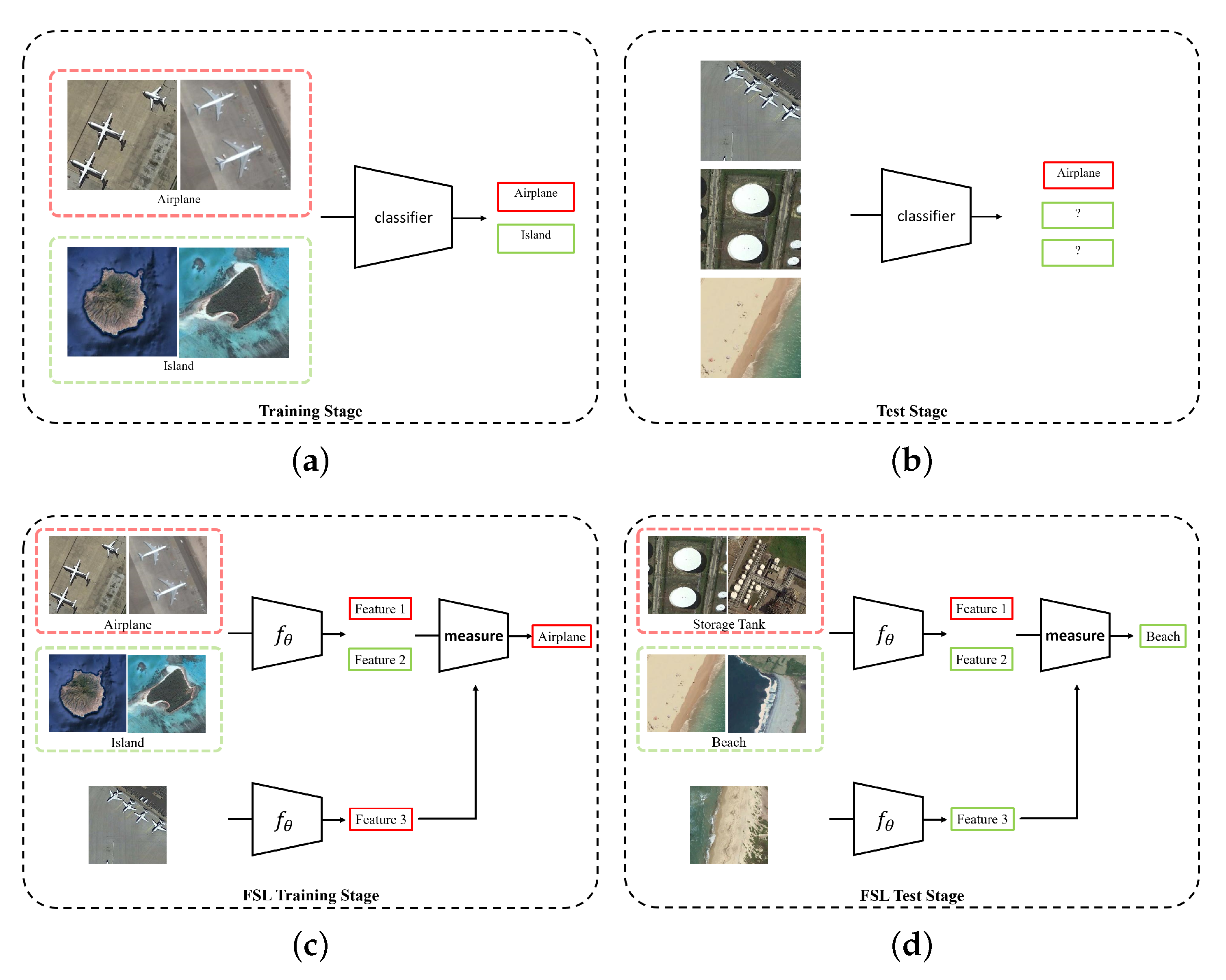Because of the particularity of remote sensing images, it is very difficult and time-consuming to obtain abundant manually annotated high-resolution remote sensing images [21], especially for unusual scenes such as military installations. Therefore, the RSISC problem in the case of a few labeled samples has become an urgent and important task to be studied. Thirdly, most of the existing DNN-based classification methods can only classify the scenes which have been trained already, but they cannot classify the untrained scenes, as shown in Figure 1. When recognizing an untrained scene by a DNN model, we need a large number of scene images to retrain the model, or fine-tune the model on new scene images. The problems mentioned above are essentially caused by the fact that deep learning methods severely rely on the training data. Due to the increasing number of remote sensing images worldwide, the highly complex geometrical structures and spatial patterns and the diversity of image features all pose a great challenge to the RSISC tasks. It is significant to find a way to learn the knowledge from just a few labeled scene images or even one image, which will greatly promote the use of remote sensing images in more fields.

In this paper, we propose a new framework to solve the one-shot RSISC problem inspired by few-shot learning (FSL) methods. The metric-based FSL method first extracts the features of labeled samples and unlabeled samples, and then classifies unlabeled samples by measuring the similarity of features. It adopts task-based methods [22] to achieve the ability to perform classification tasks that only require a small number of labeled data, even for categories that have not appeared in the training stage. For an FSL task which contains N categories of data, task-based learning does not care about the specific categories of labeled samples but focuses on the feature similarity of the unlabeled samples and classifying them to N groups. This approach makes FSL more general for different types of samples. Thus, for images from unknown classes, the few-shot classification can also be realized.

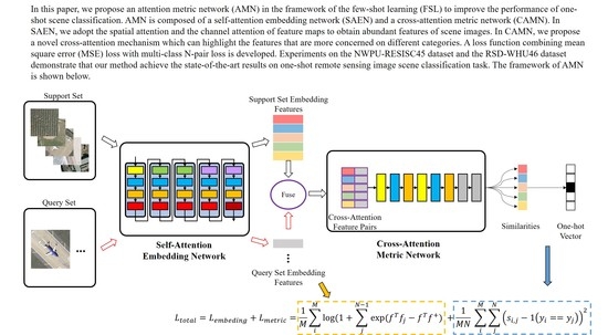
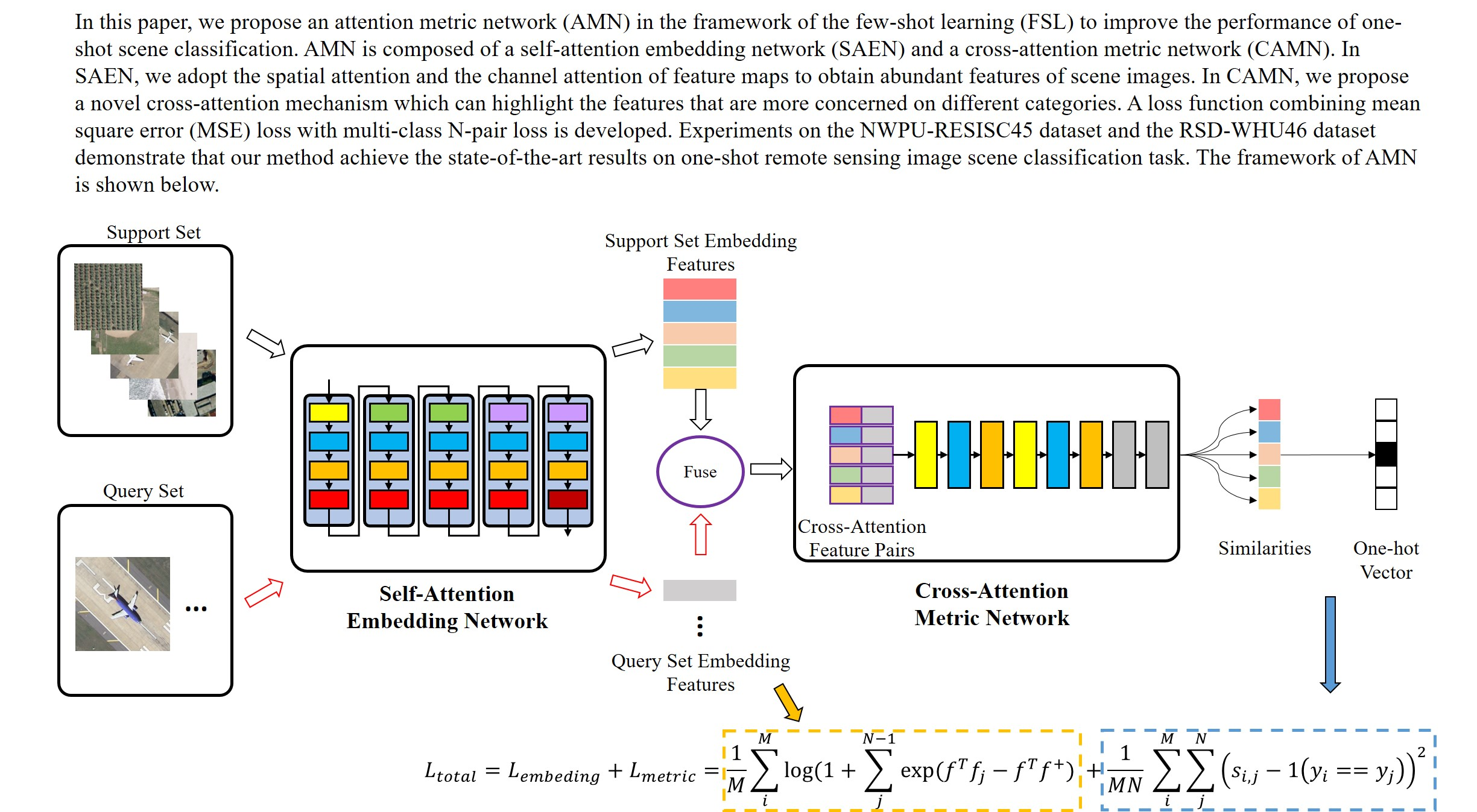
Although the FSL method has the ability of classification with only a few labeled samples, its accuracy is still far from satisfactory compared with the DNN-based method. In this paper, we design an Attention Metric Network (AMN) for one-shot RSISC to boost the performance of extracting discriminative features from a small number of labeled samples and measure the similarity of features. Specifically, we design a Self-Attention Embedding Network (SAEN) for feature extraction and a Cross-Attention Metric Network (CAMN) for similarity measurement. The SAEN applies spatial attention and channel attention to feature maps of different sizes and a different number of channels to enhance the feature extraction capabilities of different scene images. Motivated by the fact that the important features of the same category are similar, CAMN is carefully designed to extract the channel attention of the labeled embedding features and fuses with the unlabeled features. Then, CAMN measures the similarity between the fused embedding features of unlabeled samples and labeled samples to obtain the predicted class. Moreover, we use a loss function that fuses mean square error (MSE) and multi-class N-pair loss to enhance the effectiveness of AMN in one-shot scene classification tasks.

The contributions of this paper can be summarized as follows:

• We propose a metric-based FSL method AMN to solve the one-shot RSISC task. We design the SAEN in feature extraction stage and the CAMN in the similarity measurement stage for the one-shot RSISC task. The SAEN adopts both spatial and channel attention, and is carefully designed to obtain distinctive features under small labeled sample settings. The CAMN contains a novel and effective cross-attention mechanism to enhance features of interest to different categories and suppress unimportant features.
• Joint MSE loss and the multi-class N-pair loss have been developed for the one-shot RSISC task. The proposed loss function can promote the intra-class similarity and inter-class variance of embedding features and improve the accuracy of similarity metric results by the CAMN.
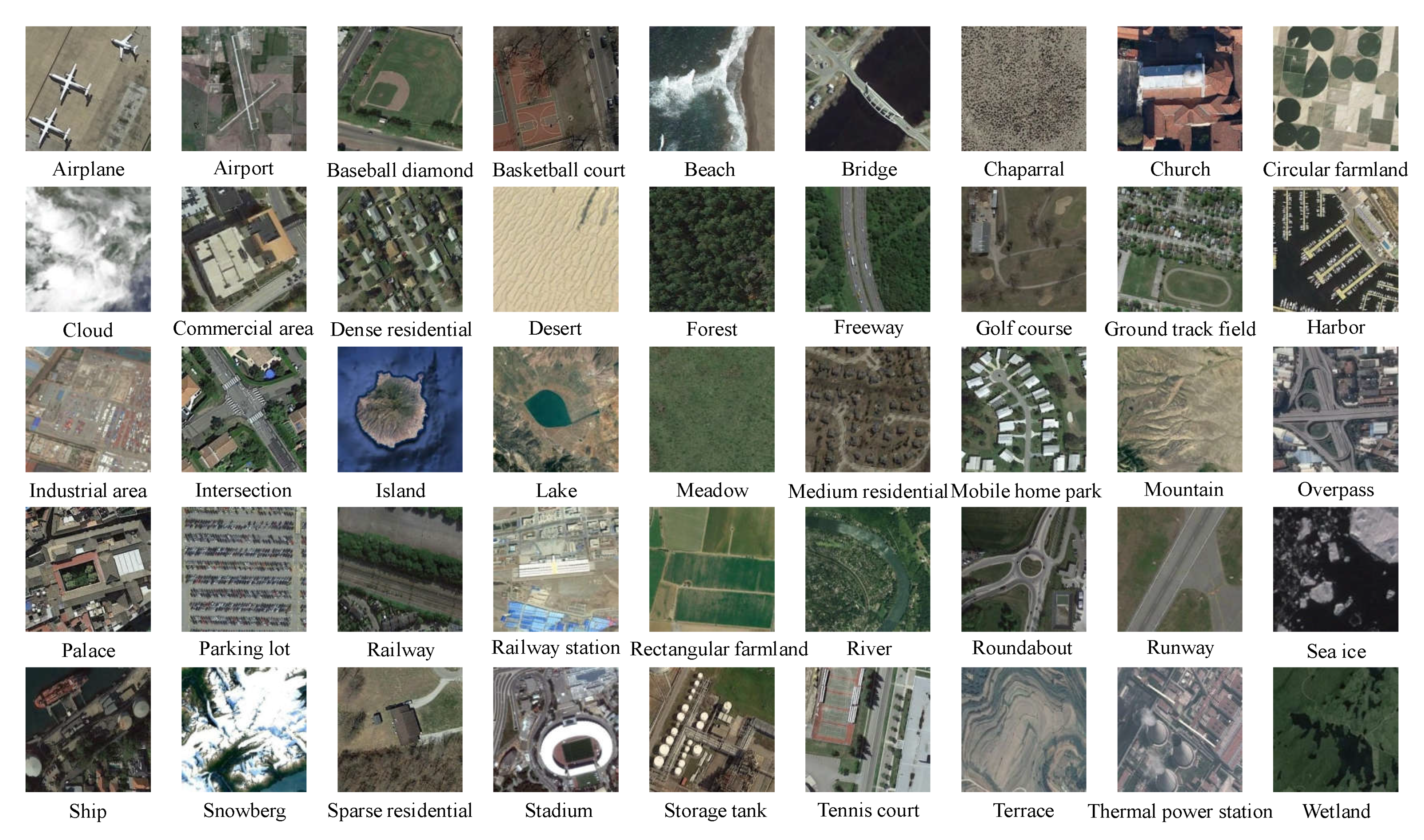
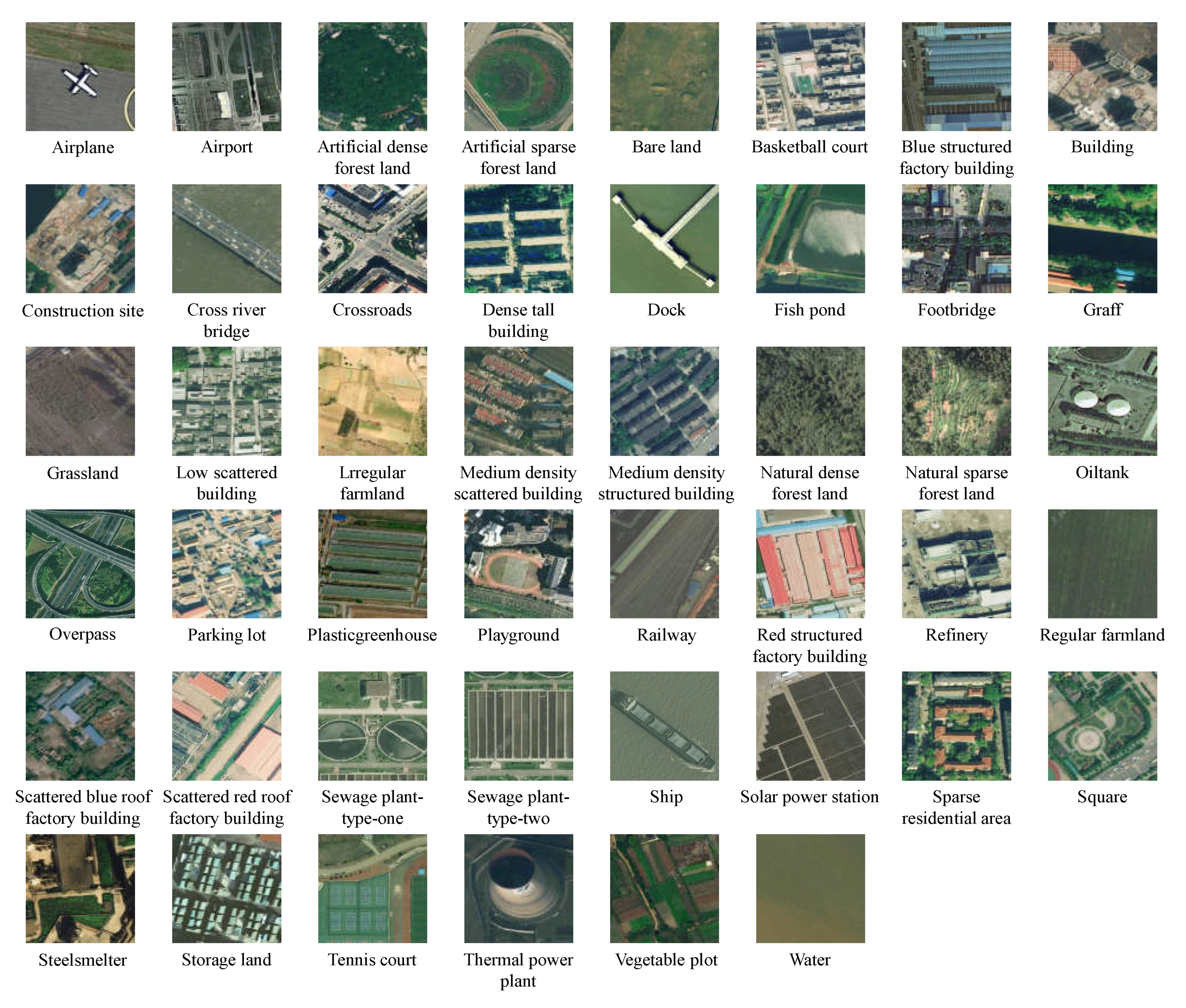
• We conduct extensive experiments on two large-scale scene classification datasets NWPU-RESISC45 [23] and RSD46-WHU [24,25]. Experimental results prove that our method can effectively promote the accuracy of the one-shot RSISC task than other state-of-the-art methods.

The rest of this paper is organized as follows. In Section 2, methods related to this paper are introduced. Detailed descriptions of the proposed method are covered in Section 3. Experiments and analysis are introduced in Section 4. In Section 5, we conduct ablation studies to prove that the contributions are all valid and further discuss the embedding features and the cross-attention mechanism. Finally, the conclusions are drawn in Section 6.

2. Related Work

In this section, we briefly review the related work of RSISC and introduce the attention mechanism and some metric-based FSL methods.

2.1. Scene Classification Methods

RSISC methods can be divided into three categories according to different feature extraction methods: handcrafted-features based methods, unsupervised-learning based methods, and deep-learning based methods [23].

Handcrafted features [10,11] are all manually extracted features, so the feature extraction methods designed by humans greatly affect the performance of feature expression. Unsupervised learning features [5,12,13,14,15] do not need labeled information of data but extract useful feature information from images by learning a basic function or filter for feature coding.

With the development of deep learning, DNN-based methods are now the dominant solutions to the RSISC problem [16,17,18,19]. DNN models are widely developed to extract more information of attention [18,26,27] and patterns [16,17] on scene images, and designed to fuse different types of patterns [17,28] to achieve better performance on RSISC tasks. Guo et al. [27] proposed a global-local attention network to improve the scene classification performance by learning the global information and the local semantic information. Anwer et al. [17] proposed a TEX-Nets fusing texture coded mapped images with the normal RGB images. Benefiting from the powerful ability of automatic learning with category tags, deep learning models can extract hierarchical and discriminate features of different scenes better than handcrafted features and unsupervised features. Therefore, we chose the DNN-based model as the backbone of our AMN method to solve the one-shot RSISC task.

2.2. Attention Mechanism

The basic idea of the attention mechanism is to highlight important information and characteristics. In the field of remote sensing, saliency detection is usually adopted to obtain regions of interest. For example, Zhang et al. [29] proposed a saliency guided sampling strategy to extract features without redundant information from remote sensing images. Zhang et al. [30] extracted the saliency feature map of primary objects as an additional encoding feature of the classifier.

With the development of deep learning, the attention mechanism is not limited to focus on the important areas of the image. Jie et al. proposed SE-Net [31] to draw attention to the channel of features in order to obtain more critical channel feature information. SangHyun et al. proposed the CBAM [32] module, which draws attention to channels and spatials of feature maps, respectively, and integrates the two attention maps into residual modules [33].

Recently, many DNN-based scene classification methods have adopted complex attention mechanisms [18,26,27]. The attention mechanisms applied in these works have effectively improved the feature expression ability of DNN in different scene images. Inspired from the existing self-attention methods, the spatial attention and the channel attention are adopted on different size and different numbers of channels of feature maps. Besides the self-attention mechanism, we proposed a novel cross-attention mechanism to enhance the ability of feature expression of specific target categories, so as to obtain better similarity measurement results.

2.3. Metric-Based Few-Shot Learning

With the development of deep learning, the metric-based FSL method has been widely applied in image classification [22,34,35], object detection [36,37], and other fields [38,39,40].

A fundamental metric-based FSL method is Matching Network (MatchingNet) [22]. In this paper, Vinyal et al. for the first time raised task-based FSL training and testing mode N-way K-shot. An N-way K-shot task contains N categories of data, in which the data of each category include K labeled samples (called support sets) and Q unknown samples (called query sets). Different from the traditional classification task, the N-way K-shot task predicts the label of the query set sample by matching the feature of the query set sample with that of the support set sample.

Snell et al. [34] proposed prototypical network (ProtoNet). The ProtoNet finds the centers of K labeled support set features as the prototype of the category. By calculating the L2 distance between unlabeled samples and different prototypes, the predicted category is the label of the nearest prototype. On the basis of the prototype network, Sung et al. proposed the relation network (RelationNet) [35]. RelationNet uses a neural network to replace the L2 distance in the ProtoNet and directly outputs the predicted category results.

Recently, metric-based FSL methods have been applied in the field of remote sensing. Liu et al. [41] applied the metric-based FSL method to hyperspectral image classification. They used a 3D-CNN to extract features from hyperspectral images and measured the similarity of labeled sample features and unlabeled sample features by Euclidean distance. Tang et al. [42] proposed an improved Siamese network to solve the few-shot SAR target detection problem. Gao et al. [43] designed a new deep classification model based on the relation network for hyperspectral image few-shot classification applications. Cheng et al. [44] applied the idea of meta learning to scene classification first and they proposed a D-CNN to solve the few-shot scene classification problems. Zhang et al. [45] proposed a state-of-the-art meta-learning method to solve a few-shot RSISC problem. They modified the ProtoNet and used the cosine distance as a similarity metric, and got 69.46% and 69.08% accuracy on a one-shot RSISC task on NWPU-RESISC45 and the RSD46-WHU datasets.

Although these works verify the applicability of FSL in the field of remote sensing, there is still a huge potential for improvement. There are two key problems in the metric-based FSL method: extract significant features from a small number of labeled samples, and measure the similarity of features. Our works are aiming to solve these problems more effectively, and to improve one-shot scene classification performance. Thus, we combine the attention mechanism with the metric-based FSL method, and propose an AMN to improve the classification results of one-shot RSISC tasks.

3. Method Description

In this section, we introduce the architecture and settings of AMN for the one-shot RSISC task in detail.

3.1. Overall Architecture

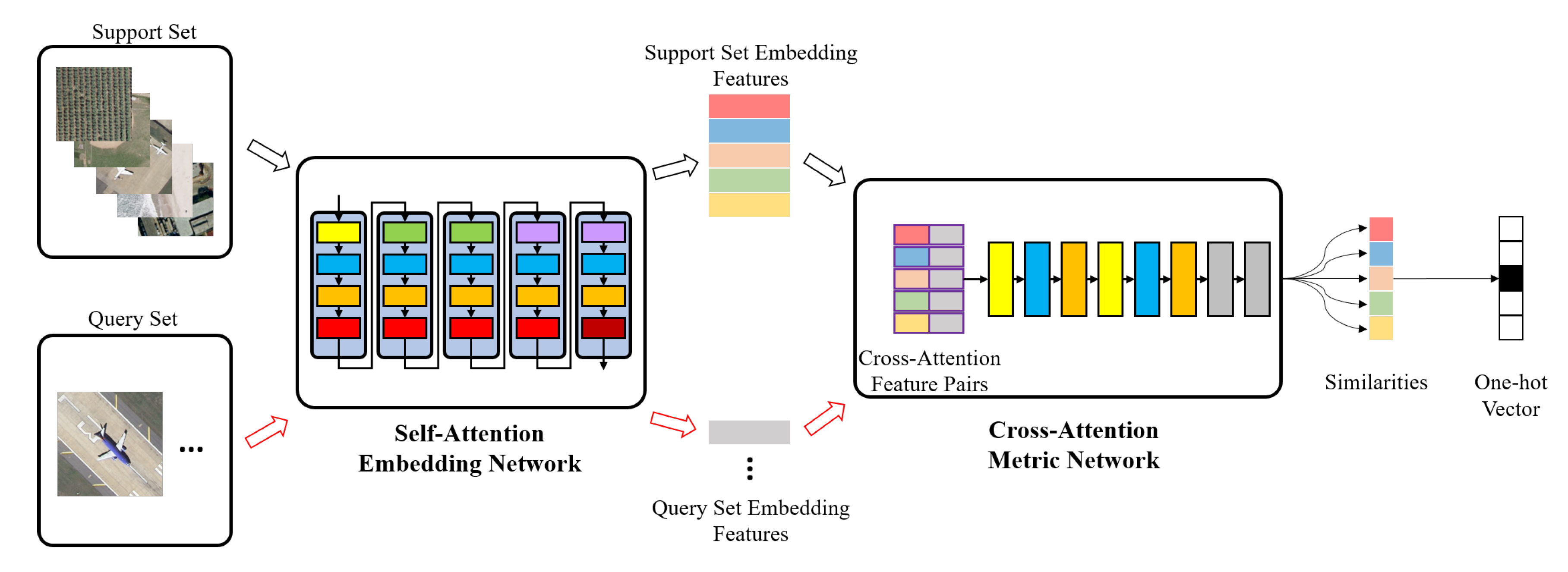
AMN is mainly composed of two parts: SAEN and CAMN. The overall framework of the AMN algorithm is shown in Figure 2.

We apply AMN to the 5-way 1-shot scene classification task. During the training stage, we randomly select 5-way 1-shot tasks from the training data. Each task contains five categories of images, and each category includes one support set image and 15 query set images. The embedding features of five labeled samples (from support set) and 75 query samples (from query set) are calculated by SAEN. Then, CAMN is used to measure the similarities among 75 query set embedding features and five support set embedding features. Each query set image will get five similarity measurement results, and the class of the most similar support set image is the predicted label. In the testing phase, we randomly select tasks from the test data that differ from the scene categories in the training stage.

3.2. Self-Attention Embedding Network

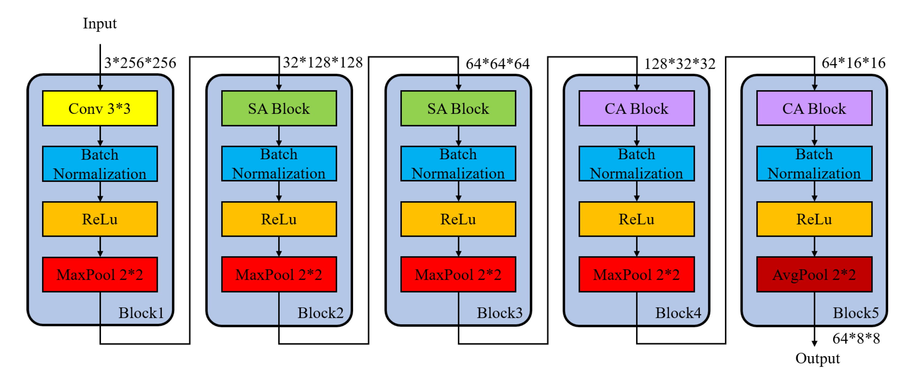
The SAEN is composed of five blocks, which is shown in Figure 3. The size of input image is $3\times 256\times 256$, and the shape of output embedding features of SAEN is $64\times 8\times 8$.

The spatial attention is applied in the second and third block of SAEN due to the large scale of feature map. In addition, the channel attention is adopted in the fourth and fifth blocks of SAEN for the rich information of channel dimensions.

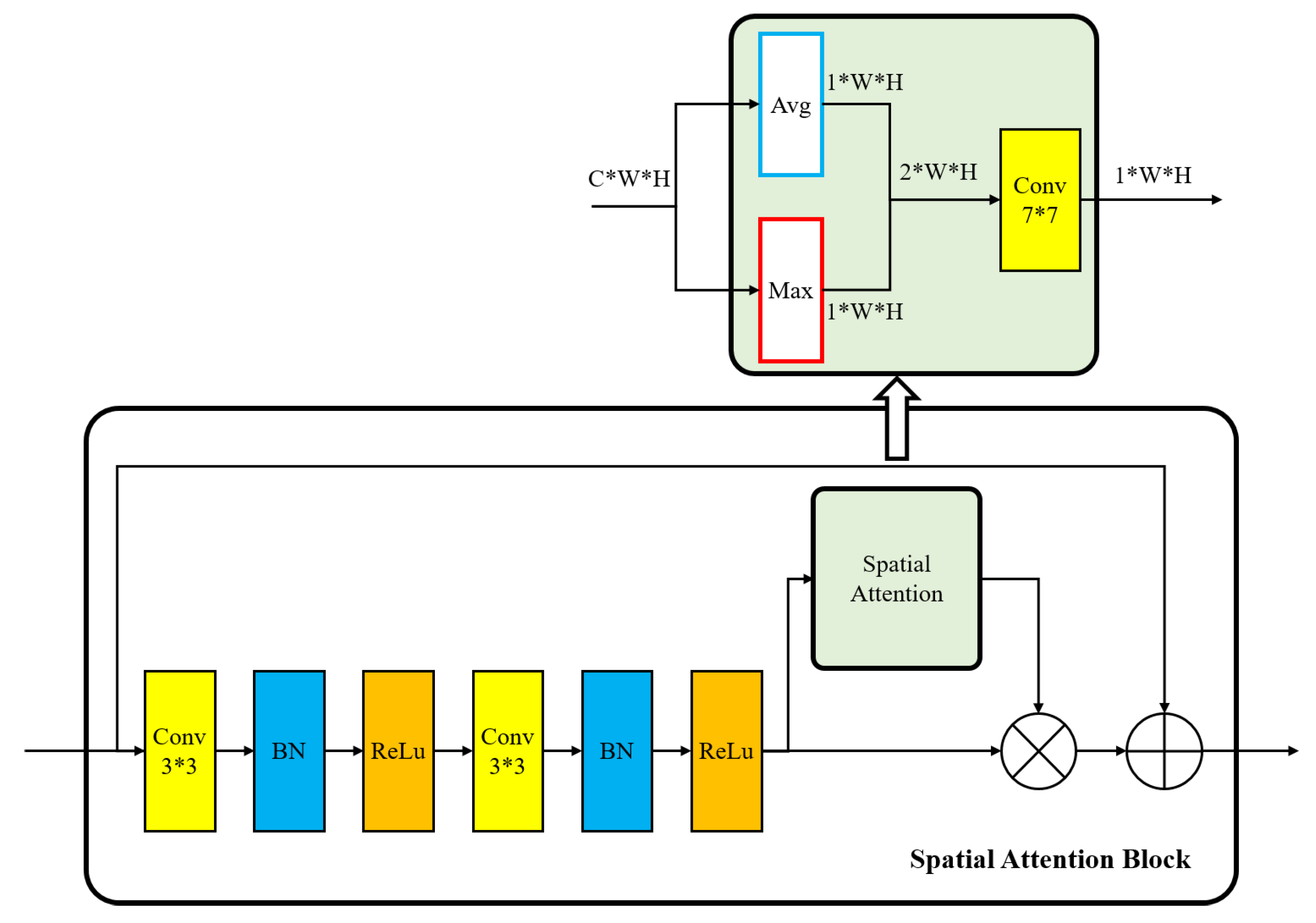
We extract the spatial attention map in the second and third blocks of SAEN. The spatial attention block is shown in Figure 4. We calculate the average value $Avg\left(\mathit{F}\right)$ and the maximum value $Max\left(\mathit{F}\right)$ of the channel on a $C\times W\times H$ size feature map $\mathit{F}$, and obtain two $1\times W\times H$ size feature maps ${\mathit{F}}_{\mathit{avg}}^{\mathit{s}}$, ${\mathit{F}}_{\mathit{max}}^{\mathit{s}}$ and concatenate them together. Then, a $7\times 7$ convolution layer is used to get a single channel spatial attention feature map with the same input size as $1\times W\times H$.

The spatial attention can be calculated as

$$\begin{array}{cc}\hfill {\mathit{M}}_{\mathit{s}}\left(\mathit{F}\right)& =\sigma \left(con{v}^{7\times 7}\left([Avg\left(\mathit{F}\right);Max\left(\mathit{F}\right)]\right)\right)\hfill \\ \hfill & =\sigma \left(con{v}^{7\times 7}\left([{\mathit{F}}_{\mathit{avg}}^{\mathit{s}};{\mathit{F}}_{\mathit{max}}^{\mathit{s}}]\right)\right)\hfill \end{array}$$

(1)

where $con{v}^{7\times 7}$ denotes a convolutional operation with a $7\times 7$ size filter, and $\sigma$ represents the sigmoid activation function.

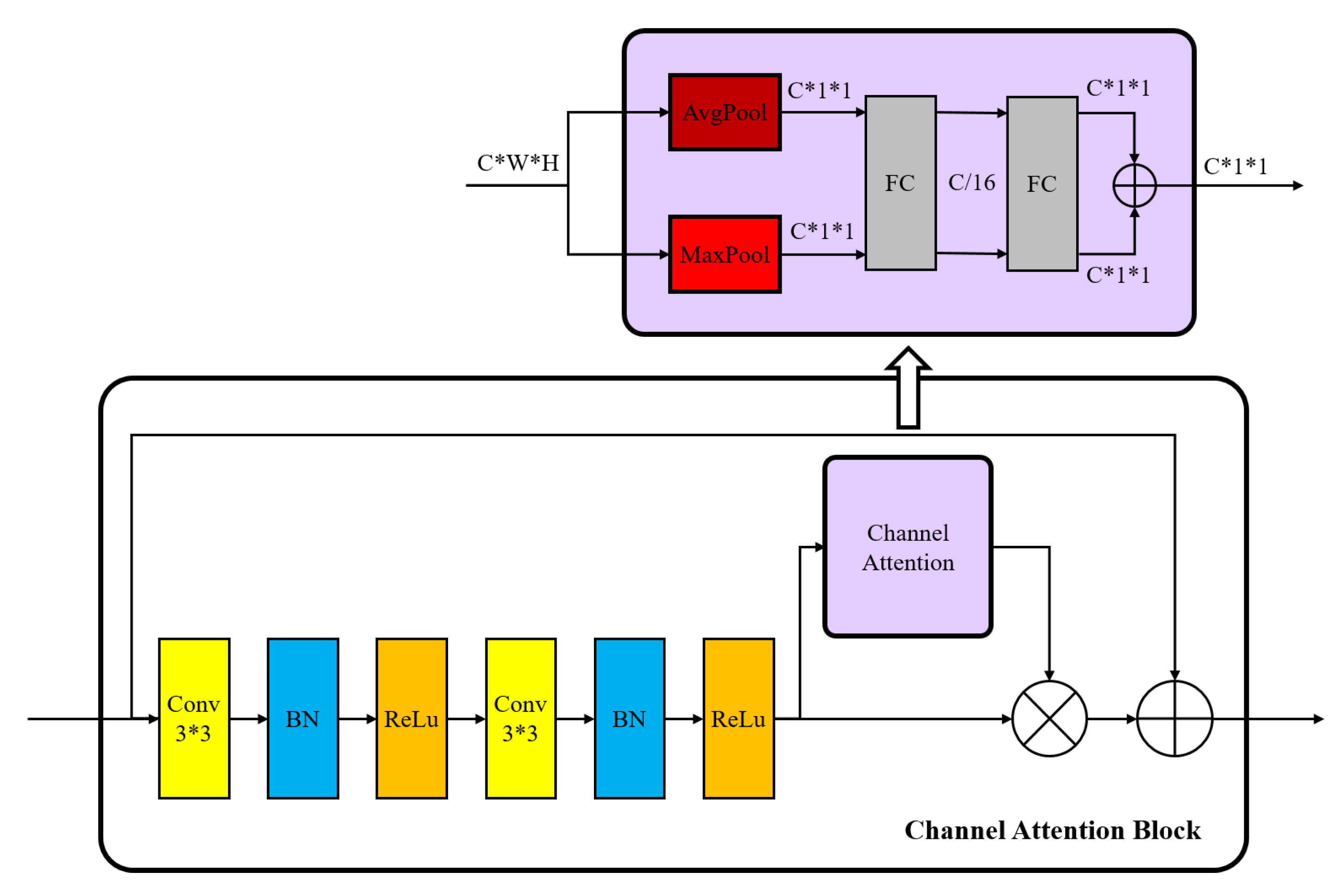
We extract the channel attention map in the fourth and fifth block of SAEN. The channel attention block is shown in Figure 5. We calculate the average value and maximum value on the $C\times W\times H$ size feature map, and obtain two $C\times 1\times 1$ size features. Then, two feature maps are added through two fully connected layers to get the channel attention feature map with the size of $C\times 1\times 1$.

The channel attention can be calculated as

$$\begin{array}{cc}\hfill {\mathit{M}}_{\mathit{c}}\left(\mathit{F}\right)& =\sigma \left(MLP\right(AvgPool\left(\mathit{F}\right))+MLP(MaxPool\left(\mathit{F}\right)\left)\right)\hfill \\ \hfill & =\sigma ({\mathit{W}}_{\mathbf{1}}\left({\mathit{W}}_{\mathbf{0}}\left({\mathit{F}}_{\mathit{avg}}^{\mathit{c}}\right)\right)+{\mathit{W}}_{\mathbf{1}}\left({\mathit{W}}_{\mathbf{0}}\left({\mathit{F}}_{\mathit{max}}^{\mathit{c}}\right)\right))\hfill \end{array}$$

(2)

where $\sigma$ represent the sigmoid function, fully connected layer weights ${\mathit{W}}_{\mathbf{0}}\in {\mathbb{R}}^{C/r\times C}$ and ${\mathit{W}}_{\mathbf{1}}\in {\mathbb{R}}^{C\times C/r}$ are shared for both inputs, and the ReLU activation function is followed by ${\mathit{W}}_{\mathbf{0}}$.

By using the spatial attention block and channel attention block, the SAEN can extract more abundant spatial and channel attention features, and then promote the feature expression ability of SAEN.

3.3. Cross-Attention Metric Network

We design the CAMN to improve the ability of metric networks to distinguish embedding features of the same categories and different categories. The cross-attentive mechanism is inspired by the fact that the channel attention of embedding features is more similar for the same class. When we aggregate the channel attention of different support set image features with a query set image features, the metric network can easily distinguish the class of the query set image.

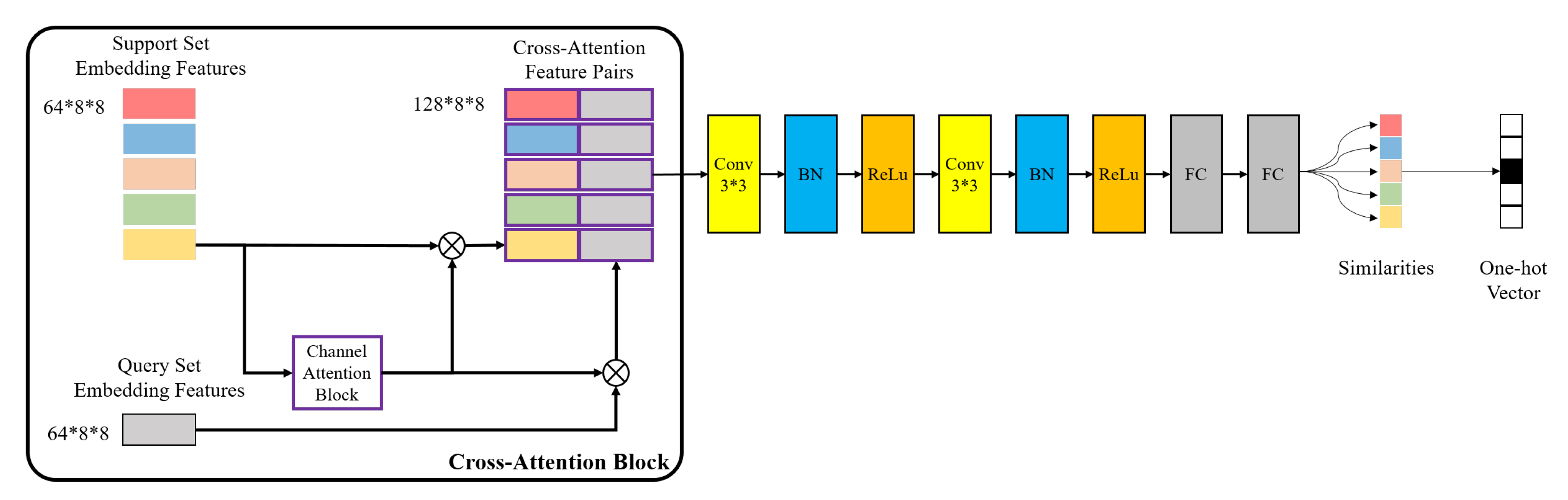
The CAMN contains a cross-attention block and a metric network, which is shown in Figure 6.

In the cross-attention block, we firstly calculate the channel attention for embedding features of each support set image. Then, we fuse the channel attention with support embedding features and query embedding features respectively, and concatenate them by channel dimensions to form a $128\times 8\times 8$-dimensional feature pair. The channel attention and fused features are calculated the same way as the channel attention module in Section 3.2. In a 5-way 1-shot task, each query sample can get five feature pairs, so a total of $75\times 5=375$ pairs of cross attention features are obtained.

The metric network consists of two Conv-BN-ReLu layers and two fully connected layers. The kernel size of convolutional layer is $3\times 3$, padding is 0, and stride is 1. The output sizes of the first and second full connection layer are 8 and 1, respectively. Finally, the similarity of each feature pair is obtained through sigmoid functions. The category with the largest similarity is the prediction category. Thus, each query set image would get a five-dimensional one-hot vector, representing the predicted result.

Suppose the cross-attention metric network is $g_{metric}$, the embedding features of a query image x is $F_x$, the embedding features of a sample image i is $F_i$, and its channel attention is $C{A}_{F_i}$. Then, the mathematical processing of the similarity of $F_x$ and $F_i$ and the predicted category of query set x can be expressed as:

$$S_i=g_{metric}({\mathit{CA}}_{{\mathit{F}}_{\mathit{i}}}\times {\mathit{F}}_{\mathit{x}},{\mathit{CA}}_{{\mathit{F}}_{\mathit{i}}}\times {\mathit{F}}_{\mathit{i}})i=1,2,3,4,5$$

(3)

$$Y_{pred}=\underset{i}{argmax}\left(S_i\right)i=1,2,3,4,5$$

(4)

3.4. Loss Function

To improve the intra-class similarity and the inter-class variance, we adopt MSE loss in the measurement part, and use multi-class N-pair loss [46] in the feature extraction stage to expand the difference of embedding features between different categories.

In contrast to traditional scene classification tasks, we use similarity to predict the category of unlabeled images in the FSL scenario. We train our model using mean square error (MSE) loss by regressing the similarity scores on groundtruth: matching feature pairs have a similarity of 1, and mismatched pairs have a similarity of 0. The MSE loss can described as follows:

$$L_{metric}=\frac{1}{MN}\sum _i^M\sum _j^N{(s_{i,j}-1(y_i==y_j))}^2$$

(5)

where $y_i$ denotes the label of query image i, $y_j$ denotes the label of sample image j, and $s_{i,j}$ represents the output similarity of the feature pairs of i and j through the CAMN.

For each query sample, we use the vector inner product to measure the distance between positive samples of the same classes and negative samples of different classes in the feature embedding stage. The expression of multi-class N-pair loss is as follows:

$$L_{embedding}=\frac{1}{M}\sum _i^{M}log(1+\sum _j^{N-1}exp({\mathit{f}}^T{\mathit{f}}_{\mathbf{j}}-{\mathit{f}}^T{\mathit{f}}^{+}))$$

(6)

where $\mathit{f}$ represents the embedding features of query set i, ${\mathit{f}}_{\mathbf{j}}$ denotes embedding features of the negative support set image j whose class is different with i, and ${\mathit{f}}^{+}$ represents the embedding features of positive support set image which is the same as i.

To sum up, the total loss function is:

$$\begin{array}{cc}\hfill L_{total}& =L_{metric}+L_{embedding}\hfill \\ \hfill & =\frac{1}{MN}\sum _i^M\sum _j^N{(s_{i,j}-1(y_i==y_j))}^2+\frac{1}{M}\sum _i^{M}log(1+\sum _j^{N-1}exp({\mathit{f}}^T{\mathit{f}}_{\mathit{j}}-{\mathit{f}}^T{\mathit{f}}^{+}))\hfill \end{array}$$

(7)

4. Experiments and Results

In this section, we introduce datasets and experimental settings. Then, we compare the results of some state-of-the-art methods and our proposed method on two commonly used RSISC datasets.

4.1. Experiment Datasets and Experiment Setup

4.1.1. Datasets Description

In order to verify the effectiveness of our method in one-shot remote sensing scene classification, we conducted a number of experiments on two large-scale RSISC datasets, the NWPU-RESISC45 dataset and the RSD46-WHU dataset.

The NWPU-RESISC45 dataset contains 45 kinds of scene images, each class contains 700 images with the size of $256\times 256$, a total of 31,500 images. These images are intercepted from remote sensing images taken by satellites in Google maps. Most of the scene images have pixel resolution between 0.2 and 30 m, and a few have lower spatial resolutions. Figure 7 shows sample images for each category in the NWPU-RESISC45 dataset.

RSD46-WHU is a large-scale open dataset for remote sensing image scene classification. This dataset is collected from Google Earth and Tianditu and contains 46 classes, each with 500–3000 images, for a total of 117,000 images. The ground resolution of most classes is 0.5 m and that of others is about 2 m. The dataset is divided into training set and validation set. We use the training set for experiments, about 99,000 images. Figure 8 shows sample images for each category in the RSD46-WHU dataset.

It should be noted that some categories of scene images have large intra-class variance and high inter-class similarity, which greatly increases the difficulty of classification.

4.1.2. Experiment Settings

In each dataset, we randomly select five categories as the test data for the 5-way 1-shot task, and other categories as the training data. In order to verify the reliability of our method, we repeat five experiments on each dataset and select different test categories each time. We compared our method with two typical metric-based FSL methods ProtoNet and RelationNet to prove the superiority of our method.

In the preprocessing stage, the image is resized to $256\times 256$, and the training image is randomly flipped vertically or horizontally with a 50% probability and normalized. In the training stage, 5-way 1-shot tasks were randomly selected from the training data and divided into 800 epochs, each epoch contained 200 tasks, a total of 160,000 tasks. A 5-way 1-shot task contains five categories, each containing one support set image and 15 query set images. We use the SGD optimizer to update the network parameters. The initial learning rate is 1 × 10⁻³, the momentum is 0.9, and the regularization coefficient is 5 × 10⁻³. After each epoch training, 150 5-way 1-shot tasks are randomly selected from the test categories for verification, and the network weight with the highest test accuracy is retained as the final result. In the test phase, we randomly selected 600 5-way 1-shot tasks from testing data to test and evaluate.

The PyTorch framework is used to implement the proposed method. All the implementations are evaluated on a Ubuntu 16.04 system with one 3.6 GHz 4-core i7-7700CPU, 64 GB memory and a GPU of NVIDIA GTX 1080ti.

4.1.3. Evaluation Metrics

We use three metrics to evaluate our experimental results, including average accuracy, 95% confidence interval, and confusion matrix.

• Average accuracy: the ratio of the number of correctly classified samples to the number of all samples in 600 5-way 1-shot tasks.
• 95% confidence interval: the probability that the classification accuracy of a 5-way 1-shot task falls within this interval is 95%.
• Confusion matrix: each column of the matrix is the predicted category, and each row of the matrix is the real category. In each group of experiments, 600 5-way 1-shot tasks were counted. Each task contains 75 query set, including 45,000 samples in total.

4.2. Experimental Results on the NWPU-RESISC45 Dataset

We conducted five groups of experiments on the NWPU-RESISC45 dataset. In each experiment, we select 40 categories of images as the training set, and the remaining five categories of the images as the test set. The experiment number and test categories are shown in

Table 1. Test categories and examples in each experiment on the NWPU-RESISC45 dataset.

Experiment	Test Categories	Example Images
1	Storage tank; Tennis court; Terrace; Thermal power station; Wetland
2	Airplane; Cloud; Industrial area; Palace; Ship
3	Baseball diamond; Dense residential; Island; Railway; Sparse residential
4	Beach; Forest; Meadow; Rectangular farmland; Storage tank
5	Chaparral; Golf course; Mobile home park; Roundabout; Terrace

.

Table 2. Average accuracy(%) and 95% confidence interval(%) of ProtoNet, RelationNet and AMN on the NWPU-RESISC45 dataset, each experiment contains 600 randomly selected tasks. The best results on each experiment are marked in bold.

Experiment	ProtoNet [34]	RelationNet [35]	AMN
1	57.27 ± 0.79	59.02 ± 0.76	63.80 ± 0.72
2	50.20 ± 0.70	52.76 ± 0.77	51.37 ± 0.81
3	71.22 ± 0.66	74.14 ± 0.66	77.02 ± 0.64
4	66.27 ± 0.83	66.04 ± 0.77	73.57 ± 0.68
5	59.76 ± 0.75	61.37 ± 0.71	70.02 ± 0.71
MEAN	60.94	62.67	67.16

and Figure 9 show the experimental results of ProtoNet, RelationNet, and AMN on each test set, with the best results marked in bold. The AMN gives an average improvement of 6.22% compared with the ProtoNet and 4.49% compared with the RelationNet on five sets of experiments. Except for the average accuracy of AMN in the second experiment being 1.39% lower than that of RelationNet, AMN in the other four groups is significantly improved compared with the other two methods, and the highest group is 8.65% higher than RelationNet.

The 5-way 1-shot classification results of all the test images in each group of experiments were counted by the confusion matrix. Each experiment included 600 5-way 1-shot tasks with a total of 45,000 test images. The results of confusion matrix are shown in Figure 10. It can be seen that the recognition accuracy of different categories in each group of experiments is very similar, and there is no obvious misclassification relationship between different categories.

4.3. Experimental Results on the RSD46-WHU Dataset

We have carried out five groups of experiments on the RSD46-WHU dataset. In each experiment, we select 41 categories of images as the training set, and the remaining five categories of images as test sets. The experiment number and test categories are shown in

Table 3. Test categories and examples in each experiment on the RSD46-WHU dataset.

Experiment	Test Categories	Example Images
1	Storage land; Tennis court; Thermal power plant; Vegetable plot; Water
2	Airplane; Cross river bridge; Irregular farmland; Playground; Ship
3	Artificial dense forest land; Dense tall building; Medium density structured building; Red structured factory building; Sparse residential area
4	Bare land; Fish pond; Natural sparse forest land; Regular farmland; Steel smelter
5	Blue structured factory building; Graff; Overpass; Scattered red roof factory building; Tennis court

.

Table 4. Average accuracy(%) and 95% confidence interval(%) of ProtoNet, RelationNet and AMN on the RSD46-WHU dataset, each experiment contains 600 randomly selected tasks. The best results on each experiment are marked in bold.

Experiment	ProtoNet [34]	RelationNet [35]	AMN
1	57.73 ± 0.64	60.78 ± 0.68	69.92 ± 0.73
2	61.91 ± 0.83	64.32 ± 0.73	67.56 ± 0.79
3	52.71 ± 0.63	61.36 ± 0.60	61.28 ± 0.60
4	65.51 ± 0.69	68.21 ± 0.70	70.56 ± 0.70
5	52.71 ± 0.63	59.00 ± 0.66	67.46 ± 0.77
MEAN	58.11	62.73	67.36

and Figure 11 show the experimental results of ProtoNet, RelationNet and AMN on each test set, and the optimal results of each group are marked in bold. The AMN gives an average improvement of 9.25% compared with the ProtoNet and 4.63% compared with the RelationNet on five sets of experiments. Except for the average accuracy rate of the 5-way 1-shot task in AMN of the third group being 0.08% lower than that of RelationNet, the other four groups of experimental AMN are significantly improved compared with the other two methods, with the highest improvement of 9.14% compared with RelationNet.

The 1-shot classification results of all the test images in each group of experiments are counted by the confusion matrix. Each experiment includes 600 5-way 1-shot tasks with a total of 45,000 test images. The results of confusion matrix are shown in Figure 12. It can be seen that the recognition accuracy of different categories in each group of experiments is very similar, and there is no obvious misclassification relationship between different categories.

It can be seen from ten sets of experiments on two datasets that the AMN method developed in this paper achieves higher classification accuracy than ProtoNet and RelationNet in the 5-way 1-shot scene classification task, which proves the superiority of our method.

4.4. Further Analysis

To verify the performance of 5-way 1-shot tasks on more test categories, we carry out experiments as the same settings in paper [45]. The datasets are divided into the test set (12 categories on each dataset: Roundabout, Runway, Sea ice, Ship, Snowberg, Sparse residential, Stadium, Storage tank, Tennis court, Terrace, Thermal power station, Wetland on NWPU-RESISC45 dataset; Sewage plant-type-one, Sewage plant-type-two, Ship, Solar power station, Sparse residential area, Square, Square, Storage land, Tennis court, Thermal power plant, Vegetable plot, Water on RSD46-WHU dataset) and training set (other categories), the same as paper [45]. We randomly 600 select 5-way 1-shot tasks form test set, each containing 15 query images per category. The comparisons to other methods are shown in

Table 5. Results on two different groups of experiments. The best results on each dataset are marked in bold.

Results on the NWPU-RESISC45 Dataset
Method	One-Shot Result (%)
ProtoNet [34]	51.17 ± 0.79
RelationNet [35]	53.52 ± 0.83
MAML [47]	57.10 ± 0.82
D-CNN [44]	36.00 ± 6.31
Meta-Learning [45]	69.46 ± 0.22
AMN(Ours)	70.25 ± 0.79
Results on the RSD-WHU46 Dataset
Method	One-Shot Result (%)
ProtoNet [34]	52.57 ± 0.89
RelationNet [35]	52.73 ± 0.91
MAML [47]	55.18 ± 0.90
D-CNN [44]	30.93 ± 7.49
Meta-Learning [45]	69.08 ± 0.25
AMN(Ours)	73.2 ± 0.75

.

Our method achieves the state-of-the-art accuracy on both datasets, with about 0.79% and 4.12% increasing compared to the recent Meta-Learning [45] method.

5. Discussion

5.1. Ablation Study

Table 6. Ablation studies on two different groups of experiments.

Results on NWPU-RESISC45 Dataset
Method	Result (%)
AMN(without cross-attention)	69.66 ± 0.67
AMN(without multi-class N-pair loss)	71.86 ± 0.73
AMN	73.57 ± 0.68
Results on RSD-WHU46 Dataset
Method	Result (%)
AMN(without cross-attention)	69.31 ± 0.72
AMN(without multi-class N-pair loss)	67.16 ± 0.70
AMN	69.92 ± 0.73

shows ablation studies of the effects of cross-attention mechanism and the fused loss function on two different experiments. We randomly chose a group of experiments on each dataset (experiment 4 of NWPU-RESISC45 and experiment 1 of RSD-WHU46), and train models in 160,000 randomly selected 5-way 1-shot tasks under the same settings as Section 4.1.2. The average accuracy and 95% confidence intervals are counted on 600 tasks.

Without the cross-attention mechanism, the average accuracy of AMN decreases by about 3.91% on the first experiment and about 0.61% on the second experiment. It proves that our cross-attention mechanism contributes significantly to feature measurement results. The fused loss which combined MSE with multi-class N-pair loss gives an improvement of about 1.71% and 2.6%, proving its efficiency on one-shot RSISC tasks.

5.2. Embedding Features

To analyze whether the features extracted by our method are more unique and effective, we randomly select a training task and a test task in the first group of experiments of the NWPU-RESISC45 dataset and adopt the Principal Components Analysis (PCA) to reduce the dimension of query embedding features to 2D for visualization. Figure 13 shows the visualization results. It shows that the embedding distance of the same classes extracted by the AMN is closer, and the distance between the different classes is larger.

We utilize the Davies Bouldin index (DBI) [48] to evaluate the distance between classes and within classes. The DBI is calculated as follows:

$$DBI=\frac{1}{k}\sum _{i=1}^k\underset{i\ne j}{max}\frac{s_i+s_j}{d_{ij}}$$

(8)

where $s_i$ represents the average distance between each point of class and the centroid of that class, $d_{ij}$ denotes the distance between class centroids i and j, k represent the number of classes.

The smaller the DBI is, the smaller the intra-class distance is, and the larger the inter-class distance is.

Table 7. The DBI of embedding features on a randomly selected training set task and a randomly selected test set task. The best results on each experiment are marked in bold.

Experiment	ProtoNet	RelationNet	AMN
Training set task	0.9	1.49	0.62
Test set task	1.36	1.35	1.1

shows that the DBI of our method is the smallest of the three in both training tasks and test tasks, which proves that the features of the same category extracted by our method are more similar and the features of different categories are more different than the ProtoNet and the RelationNet.

5.3. Effectiveness of the Cross-Attention Mechanism

We randomly extract a training task and a test task from the first group of experiments on the NWPU-RESISC45 dataset, and then obtain the support set channel attention in cross-attention metric networks, and compare it with the channel attention of a randomly selected query set image, and calculate the mean absolute error (MAE) between them. The comparison results of training tasks are shown in Figure 14, and the comparison results of test tasks are shown in Figure 15.

Through the comparison, it can be seen that the MAE of the same category of channel attention is the smallest, while the different categories are larger, which means that the channel attention features of the same category are more similar. When the attention of the same kind of support set image is superimposed on the query set image, the key features of the same category will be highlighted, and when the attention of different support set images is superimposed, the key features of the different category will be weakened. Therefore, the cross-attention mechanism can promote the measurement results of the metric network.

6. Conclusions

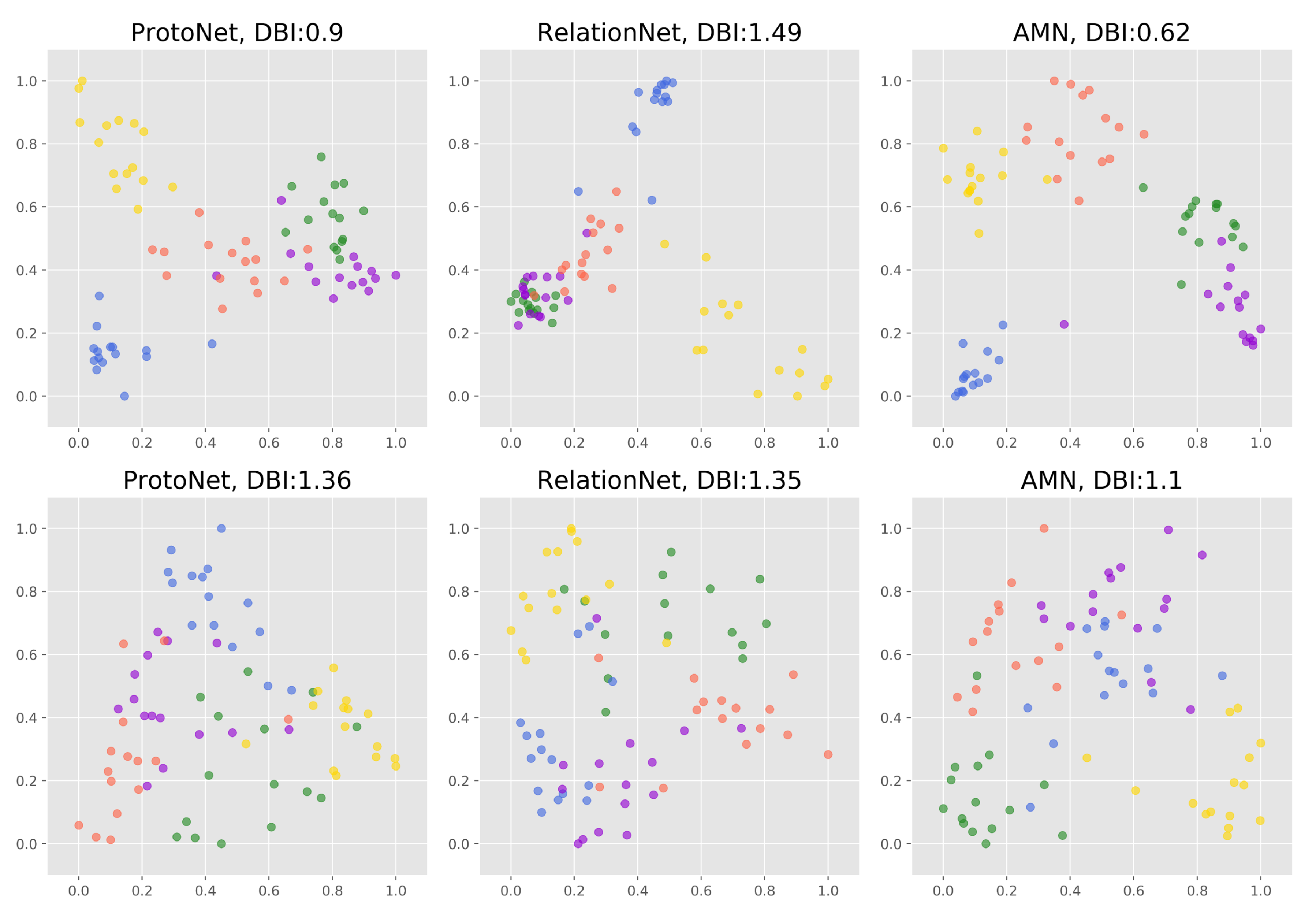
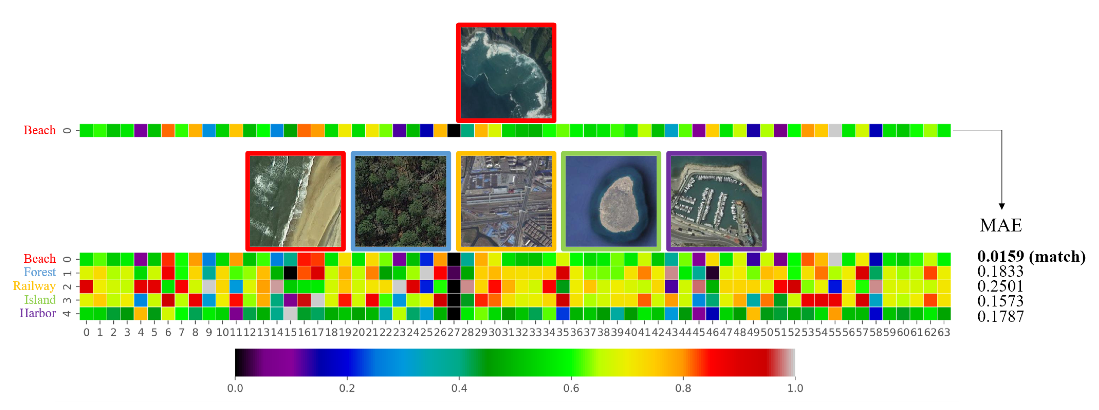
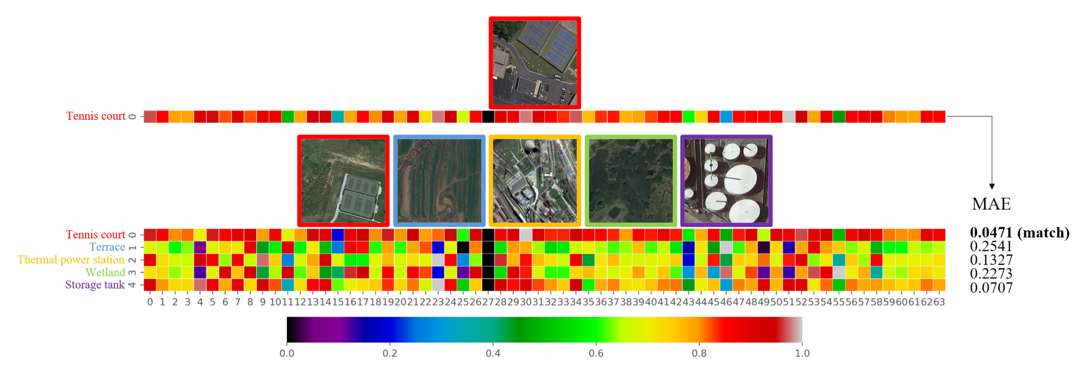
In this paper, we propose a metric-based FSL method AMN to solve the one-shot RSISC problem. To obtain more distinctive features, we design a self-attention network by using spatial attention and channel attention along with multi-class N-pair loss. The proposed AMN can extract more similar features from images of the same category and more different features among images of different categories. A novel and effective cross-attention metric mechanism is proposed in this paper. Combining unlabeled embedding features with the channel attention of the labeled features, the CAMN can highlight the features of different categories that are more concerned. The discussion about cross-attention proves that similar image features do have similar channel attention.

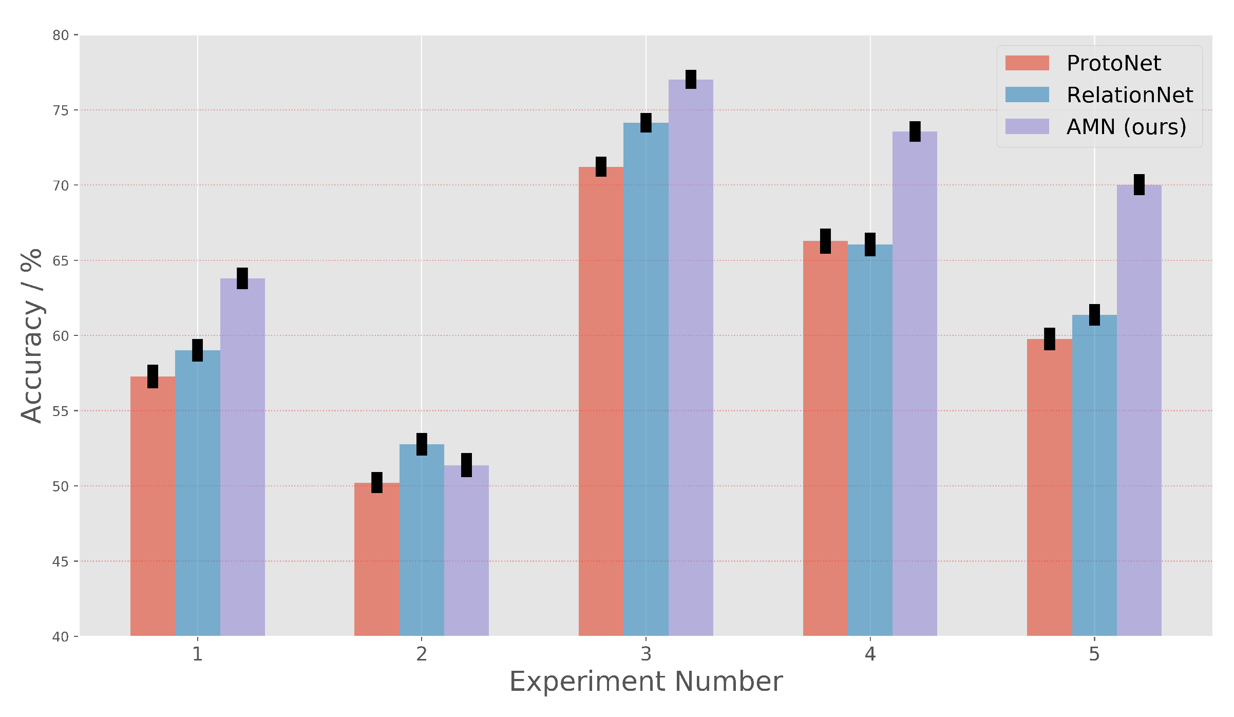
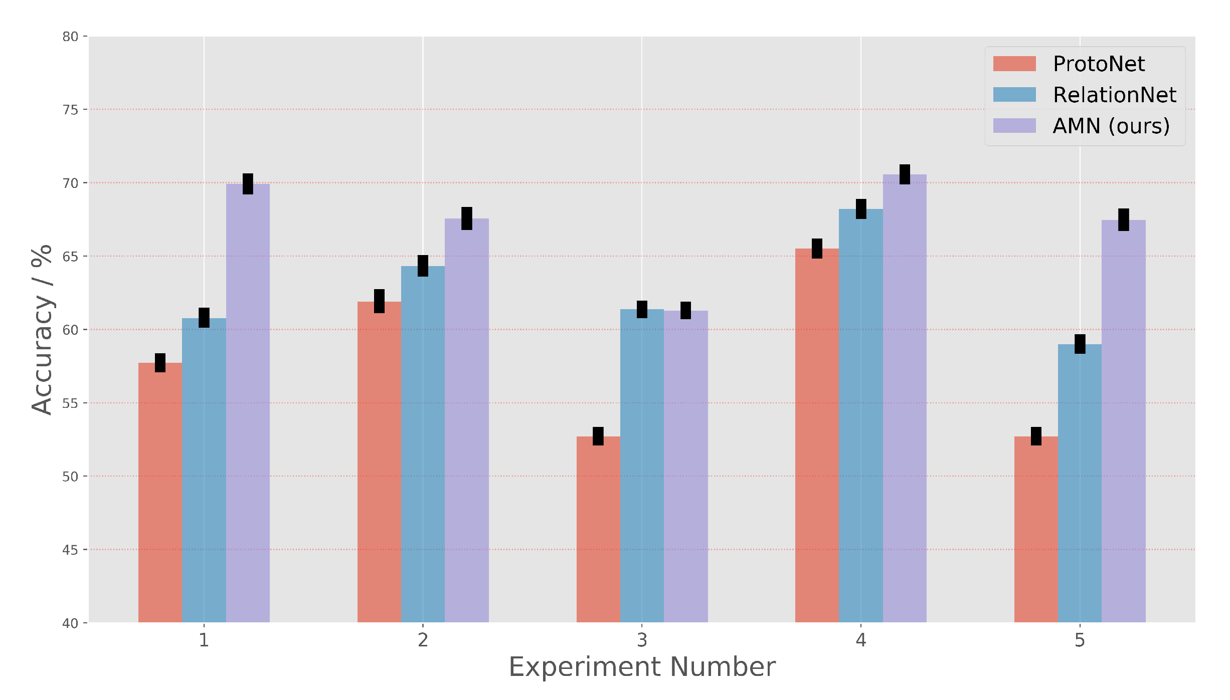
Our work achieves the state-of-the-art classification results on one-shot RSISC tasks. On the NWPU-RESISC45 dataset, the AMN achieves a gain of up to around 6.22% over the ProtoNet and about 4.49% over the RelationNet. On the RSD46-WHU dataset, the AMN method improves performance by about 9.25% to ProtoNet and about 4.63% to RelationNet. These impressive results demonstrate that not only the feature extraction method but also the cross-attention mechanism can improve the similarity measurement results of scene images, especially on one-shot RSISC tasks.

The metric-based FSL frameworks rely on a large number of different categories of scene tasks to ensure that the FSL task is category-independent. The model may over-fit to specific categories when there are few scene classes. Our future work will focus on training the FSL model on a small number of categories of scene images.

References

1. Martha, T.R.; Kerle, N.; Van Westen, C.J.; Jetten, V.G.; Kumar, K.V. Segment Optimization and Data-Driven Thresholding for Knowledge-Based Landslide Detection by Object-Based Image Analysis. IEEE Trans. Geosci. Remote. Sens. 2011, 49, 4928–4943. [Google Scholar] [CrossRef]
2. Stumpf, A.; Kerle, N. Object-oriented mapping of landslides using Random Forests. Remote Sens. Environ. 2011, 115, 2564–2577. [Google Scholar] [CrossRef]
3. Cheng, G.; Guo, L.; Zhao, T.; Han, J.; Li, H.; Fang, J. Automatic landslide detection from remote-sensing imagery using a scene classification method based on BoVW and pLSA. J. Remote. Sens. 2013, 34, 45–59. [Google Scholar] [CrossRef]
4. Helber, P.; Bischke, B.; Dengel, A.; Borth, D. EuroSAT: A Novel Dataset and Deep Learning Benchmark for Land Use and Land Cover Classification. IEEE J. Sel. Top. Appl. Earth Obs. Remote Sens. 2019, 12, 2217–2226. [Google Scholar] [CrossRef] [Green Version]
5. Zhu, Q.; Zhong, Y.; Zhao, B.; Xia, G.; Zhang, L. Bag-of-Visual-Words Scene Classifier With Local and Global Features for High Spatial Resolution Remote Sensing Imagery. IEEE Geosci. Remote. Sens. Lett. 2016, 13, 747–751. [Google Scholar] [CrossRef]
6. Cheriyadat, A.M. Unsupervised Feature Learning for Aerial Scene Classification. IEEE Trans. Geosci. Remote Sens. 2014, 52, 439–451. [Google Scholar] [CrossRef]
7. Mishra, N.B.; Crews, K.A. Mapping vegetation morphology types in a dry savanna ecosystem: Integrating hierarchical object-based image analysis with Random Forest. J. Remote Sens. 2014, 35, 1175–1198. [Google Scholar] [CrossRef]
8. Li, X.; Shao, G. Object-based urban vegetation mapping with high-resolution aerial photography as a single data source. Int. J. Remote Sens. 2013, 34, 771–789. [Google Scholar] [CrossRef]
9. Xia, G.; Hu, J.; Hu, F.; Shi, B.; Bai, X.; Zhong, Y.; Zhang, L.; Lu, X. AID: A Benchmark Data Set for Performance Evaluation of Aerial Scene Classification. IEEE Trans. Geosci. Remote Sens. 2017, 55, 3965–3981. [Google Scholar] [CrossRef] [Green Version]
10. Li, H.; Gu, H.; Han, Y.; Yang, J. Object-oriented classification of high-resolution remote sensing imagery based on an improved colour structure code and a support vector machine. Int. J. Remote Sens. 2010, 31, 1453–1470. [Google Scholar] [CrossRef]
11. Aptoula, E. Remote sensing image retrieval with global morphological texture descriptors. IEEE Trans. Geosci. Remote Sens. 2013, 52, 3023–3034. [Google Scholar] [CrossRef]
12. Yang, Y.; Newsam, S. Bag-of-Visual-Words and Spatial Extensions for Land-Use Classification. In Proceedings of the 18th SIGSPATIAL International Conference on Advances in Geographic Information Systems; Association for Computing Machinery: New York, NY, USA, 2010; pp. 270–279. [Google Scholar] [CrossRef]
13. Zhou, W.; Shao, Z.; Diao, C.; Cheng, Q. High-resolution remote-sensing imagery retrieval using sparse features by auto-encoder. Remote Sens. Lett. 2015, 6, 775–783. [Google Scholar] [CrossRef]
14. Du, B.; Xiong, W.; Wu, J.; Zhang, L.; Zhang, L.; Tao, D. Stacked convolutional denoising auto-encoders for feature representation. IEEE Trans. Cybern. 2016, 47, 1017–1027. [Google Scholar] [CrossRef] [PubMed]
15. Lu, X.; Zheng, X.; Yuan, Y. Remote sensing scene classification by unsupervised representation learning. IEEE Trans. Geosci. Remote Sens. 2017, 55, 5148–5157. [Google Scholar] [CrossRef]
16. Hu, F.; Xia, G.; Hu, J.; Zhang, L. Transferring Deep Convolutional Neural Networks for the Scene Classification of High-Resolution Remote Sensing Imagery. Remote Sens. 2015, 7, 14680–14707. [Google Scholar] [CrossRef] [Green Version]
17. Anwer, R.M.; Khan, F.S.; van de Weijer, J.; Molinier, M.; Laaksonen, J. Binary patterns encoded convolutional neural networks for texture recognition and remote sensing scene classification. ISPRS J. Photogramm. Remote Sens. 2018, 138, 74–85. [Google Scholar] [CrossRef] [Green Version]
18. Wang, Q.; Liu, S.; Chanussot, J.; Li, X. Scene classification with recurrent attention of VHR remote sensing images. IEEE Trans. Geosci. Remote Sens. 2018, 57, 1155–1167. [Google Scholar] [CrossRef]
19. Hua, Y.; Mou, L.; Zhu, X.X. Recurrently exploring class-wise attention in a hybrid convolutional and bidirectional LSTM network for multi-label aerial image classification. Isprs J. Photogramm. Remote Sens. 2019, 149, 188–199. [Google Scholar] [CrossRef]
20. Zhang, Q.S.; Zhu, S.C. Visual Interpretability for Deep Learning: A Survey. Front. Inf. Technol. Electron. Eng. 2018, 19, 27–39. [Google Scholar] [CrossRef] [Green Version]
21. Gui, R.; Xu, X.; Yang, R.; Wang, L.; Pu, F. Statistical Scattering Component-Based Subspace Alignment for Unsupervised Cross-Domain PolSAR Image Classification. IEEE Trans. Geosci. Remote. Sens. 2020, 1–15. [Google Scholar] [CrossRef]
22. Vinyals, O.; Blundell, C.; Lillicrap, T.; Kavukcuoglu, K.; Wierstra, D. Matching Networks for One Shot Learning. In Proceedings of the 30th International Conference on Neural Information Processing Systems; NIPS’16; Curran Associates Inc.: Red Hook, NY, USA, 2016; pp. 3637–3645. [Google Scholar]
23. Cheng, G.; Han, J.; Lu, X. Remote Sensing Image Scene Classification: Benchmark and State of the Art. Proc. IEEE 2017, 105, 1865–1883. [Google Scholar] [CrossRef] [Green Version]
24. Xiao, Z.; Long, Y.; Li, D.; Wei, C.; Tang, G.; Liu, J. High-resolution remote sensing image retrieval based on CNNs from a dimensional perspective. Remote Sens. 2017, 9, 725. [Google Scholar] [CrossRef] [Green Version]
25. Long, Y.; Gong, Y.; Xiao, Z.; Liu, Q. Accurate object localization in remote sensing images based on convolutional neural networks. IEEE Trans. Geosci. Remote Sens. 2017, 55, 2486–2498. [Google Scholar] [CrossRef]
26. Ji, J.; Zhang, T.; Jiang, L.; Zhong, W.; Xiong, H. Combining Multilevel Features for Remote Sensing Image Scene Classification With Attention Model. IEEE Geosci. Remote Sens. Lett. 2020, 17, 1647–1651. [Google Scholar] [CrossRef]
27. Guo, Y.; Ji, J.; Lu, X.; Huo, H.; Fang, T.; Li, D. Global-local attention network for aerial scene classification. IEEE Access 2019, 7, 67200–67212. [Google Scholar] [CrossRef]
28. Wang, G.; Fan, B.; Xiang, S.; Pan, C. Aggregating Rich Hierarchical Features for Scene Classification in Remote Sensing Imagery. IEEE J. Sel. Top. Appl. Earth Obs. Remote Sens. 2017, 10, 4104–4115. [Google Scholar] [CrossRef]
29. Zhang, F.; Du, B.; Zhang, L. Saliency-guided unsupervised feature learning for scene classification. IEEE Trans. Geosci. Remote Sens. 2014, 53, 2175–2184. [Google Scholar] [CrossRef]
30. Zhang, H.; Zhang, J.; Xu, F. Land use and land cover classification base on image saliency map cooperated coding. In Proceedings of the 2015 IEEE International Conference on Image Processing (ICIP), Quebec City, QC, Canada, 27–30 September 2015; pp. 2616–2620. [Google Scholar] [CrossRef]
31. Hu, J.; Shen, L.; Sun, G. Squeeze-and-Excitation Networks. In Proceedings of the 2018 IEEE/CVF Conference on Computer Vision and Pattern Recognition (CVPR), Salt Lake City, UT, USA, 18–23 June 2018; IEEE Computer Society: Los Alamitos, CA, USA, 2018; pp. 7132–7141. [Google Scholar] [CrossRef] [Green Version]
32. Woo, S.; Park, J.; Lee, J.Y.; Kweon, I.S. CBAM: Convolutional Block Attention Module. In Computer Vision–ECCV 2018; Ferrari, V., Hebert, M., Sminchisescu, C., Weiss, Y., Eds.; Springer International Publishing: Cham, Switzerland, 2018; pp. 3–19. [Google Scholar]
33. He, K.; Zhang, X.; Ren, S.; Sun, J. Deep Residual Learning for Image Recognition. In Proceedings of the 2016 IEEE Conference on Computer Vision and Pattern Recognition (CVPR), Las Vegas, NV, USA, 27–30 June 2016; IEEE Computer Society: Los Alamitos, CA, USA, 2016; pp. 770–778. [Google Scholar] [CrossRef] [Green Version]
34. Snell, J.; Swersky, K.; Zemel, R. Prototypical Networks for Few-shot Learning. In Proceedings of the 31st International Conference on Neural Information Processing Systems; Guyon, I., Luxburg, U.V., Bengio, S., Wallach, H., Fergus, R., Vishwanathan, S., Garnett, R., Eds.; Curran Associates Inc.: Red Hook, NY, USA, 2017; Volume 30, pp. 4077–4087. [Google Scholar]
35. Sung, F.; Yang, Y.; Zhang, L.; Xiang, T.; Torr, P.H.S.; Hospedales, T.M. Learning to Compare: Relation Network for Few-Shot Learning. In Proceedings of the 2018 IEEE/CVF Conference on Computer Vision and Pattern Recognition, Salt Lake City, UT, USA, 18–23 June 2018; pp. 1199–1208. [Google Scholar] [CrossRef] [Green Version]
36. Fan, Q.; Zhuo, W.; Tang, C.K.; Tai, Y.W. Few-Shot Object Detection with Attention-RPN and Multi-Relation Detector. In Proceedings of the 2020 IEEE/CVF Conference on Computer Vision and Pattern Recognition (CVPR), Seattle, WA, USA, 13–19 June 2020; pp. 4012–4021. [Google Scholar] [CrossRef]
37. Hsieh, T.I.; Lo, Y.C.; Chen, H.T.; Liu, T.L. One-Shot Object Detection with Co-Attention and Co-Excitation. In Advances in Neural Information Processing Systems; Wallach, H., Larochelle, H., Beygelzimer, A., Alche-Buc, F., Fox, E., Garnett, R., Eds.; Curran Associates, Inc.: Red Hook, NY, USA, 2019; Volume 32, pp. 2725–2734. [Google Scholar]
38. Han, X.; Zhu, H.; Yu, P.; Wang, Z.; Yao, Y.; Liu, Z.; Sun, M. FewRel: A Large-Scale Supervised Few-Shot Relation Classification Dataset with State-of-the-Art Evaluation. In Proceedings of the 2018 Conference on Empirical Methods in Natural Language Processing; Association for Computational Linguistics: Stroudsburg, PA, USA, 2018; pp. 4803–4809. [Google Scholar] [CrossRef] [Green Version]
39. Duan, Y.; Andrychowicz, M.; Stadie, B.; Ho, J.; Schneider, J.; Sutskever, I.; Abbeel, P.; Zaremba, W. One-Shot Imitation Learning. In Proceedings of the 31st International Conference on Neural Information Processing Systems; NIPS’17; Curran Associates Inc.: Red Hook, NY, USA, 2017; pp. 1087–1098. [Google Scholar]
40. Yang, B.; Liu, C.; Li, B.; Jiao, J.; Ye, Q.; Ye, A.; Bischof, H.; Brox, T.; Frahm, J.M. Prototype Mixture Models for Few-Shot Semantic Segmentation. In European Conference on Computer Vision; Springer International Publishing: Cham, Switzerland, 2020; pp. 763–778. [Google Scholar]
41. Liu, B.; Yu, X.; Yu, A.; Zhang, P.; Wan, G.; Wang, R. Deep few-shot learning for hyperspectral image classification. IEEE Trans. Geosci. Remote Sens. 2018, 57, 2290–2304. [Google Scholar] [CrossRef]
42. Tang, J.; Zhang, F.; Zhou, Y.; Yin, Q.; Hu, W. A Fast Inference Networks for SAR Target Few-Shot Learning Based on Improved Siamese Networks. In Proceedings of the IGARSS 2019–2019 IEEE International Geoscience and Remote Sensing Symposium, Yokohama, Japan, 28 July–2 August 2019; pp. 1212–1215. [Google Scholar] [CrossRef]
43. Gao, K.; Liu, B.; Yu, X.; Qin, J.; Zhang, P.; Tan, X. Deep relation network for hyperspectral image few-shot classification. Remote Sens. 2020, 12, 923. [Google Scholar] [CrossRef] [Green Version]
44. Cheng, G.; Yang, C.; Yao, X.; Guo, L.; Han, J. When deep learning meets metric learning: Remote sensing image scene classification via learning discriminative CNNs. IEEE Trans. Geosci. Remote Sens. 2018, 56, 2811–2821. [Google Scholar] [CrossRef]
45. Zhang, P.; Li, Y.; Wang, D.; Bai, Y. Few-shot Classification of Aerial Scene Images via Meta-learning. Preprints 2020. [Google Scholar] [CrossRef]
46. Sohn, K. Improved Deep Metric Learning with Multi-Class N-Pair Loss Objective. In Proceedings of the 30th International Conference on Neural Information Processing Systems; Curran Associates Inc.: Red Hook, NY, USA, 2016; pp. 1857–1865. [Google Scholar]
47. Finn, C.; Xu, K.; Levine, S. Probabilistic Model-Agnostic Meta-Learning. In Proceedings of the 32nd International Conference on Neural Information Processing Systems; Curran Associates Inc.: Red Hook, NY, USA, 2018; pp. 9537–9548. [Google Scholar]
48. Davies, D.L.; Bouldin, D.W. A Cluster Separation Measure. IEEE Trans. Pattern Anal. Mach. Intell. 1979, PAMI-1, 224–227. [Google Scholar] [CrossRef]
Figure 1. Comparison between the traditional CNN classification methods and metric-based FSL methods. (a,b) traditional CNN methods cannot deal with untrained classes; (c,d) metric-based FSL methods can deal with untrained classes.
Remotesensing 12 04046 g001
Figure 2. The overall framework of Attention Metric Networks.
Remotesensing 12 04046 g002
Figure 3. Self-attention embedding network.
Remotesensing 12 04046 g003
Figure 4. Spatial Attention Block. Conv: Convolutional Layer; BN: Batch Normalization Layer; ReLu: ReLU Activation Layer; Avg: Average by Channel; Max: Maximum by Channel.
Remotesensing 12 04046 g004
Figure 5. Channel Attention Block. Conv: Convolutional Layer; BN: Batch Normalization Layer; ReLu: ReLU Activation Layer; AvgPool: Average Pooling Layer; MaxPool: Maximum Pooling Layer; FC: Fully Connected Layer.
Remotesensing 12 04046 g005
Figure 6. Cross-attention metric network.
Remotesensing 12 04046 g006
Figure 7. Example images of each category in the NWPU-RESISC45 dataset.
Remotesensing 12 04046 g007
Figure 8. Example images of each category in the RSD46-WHU dataset.
Remotesensing 12 04046 g008
Figure 9. Experimental results on the NWPU-RESISC45 dataset, each experiment contains 600 randomly selected tasks.
Remotesensing 12 04046 g009
Figure 10. Confusion matrix ofAMN results on 600 randomly selected tasks on the NWPU-RESISC45 dataset. (ae) confusion matrix of text results on experiment 1–5.
Remotesensing 12 04046 g010aRemotesensing 12 04046 g010b
Figure 11. Experimental results on the RSD46-WHU dataset, each experiment contains 600 randomly selected tasks.
Remotesensing 12 04046 g011
Figure 12. Confusion matrix of AMN results on 600 randomly selected tasks on the RSD46-WHU dataset. (ae) confusion matrix of text results on experiment 1–5.
Remotesensing 12 04046 g012aRemotesensing 12 04046 g012b
Figure 13. The PCA visualization results of task extracted from the first group of experiments on the NWPU-RESISC45 dataset. Different classes are marked with different colors. Top: training set task, Bottom: test set task.
Remotesensing 12 04046 g013
Figure 14. Comparison of channel attention features of a randomly selected query set image and support set images from a training set task on the NWPU-RESISC45 dataset.
Remotesensing 12 04046 g014
Figure 15. Comparison of channel attention features of a randomly selected query set image and support set images from a test set task on the NWPU-RESISC45 dataset.
Remotesensing 12 04046 g015