Linkages between Rainfed Cereal Production and Agricultural Drought through Remote Sensing Indices and a Land Data Assimilation System: A Case Study in Morocco

 ,
,  ,
,  ,
,  ,
, 

Abstract
1. Introduction
2. Materials and Methods
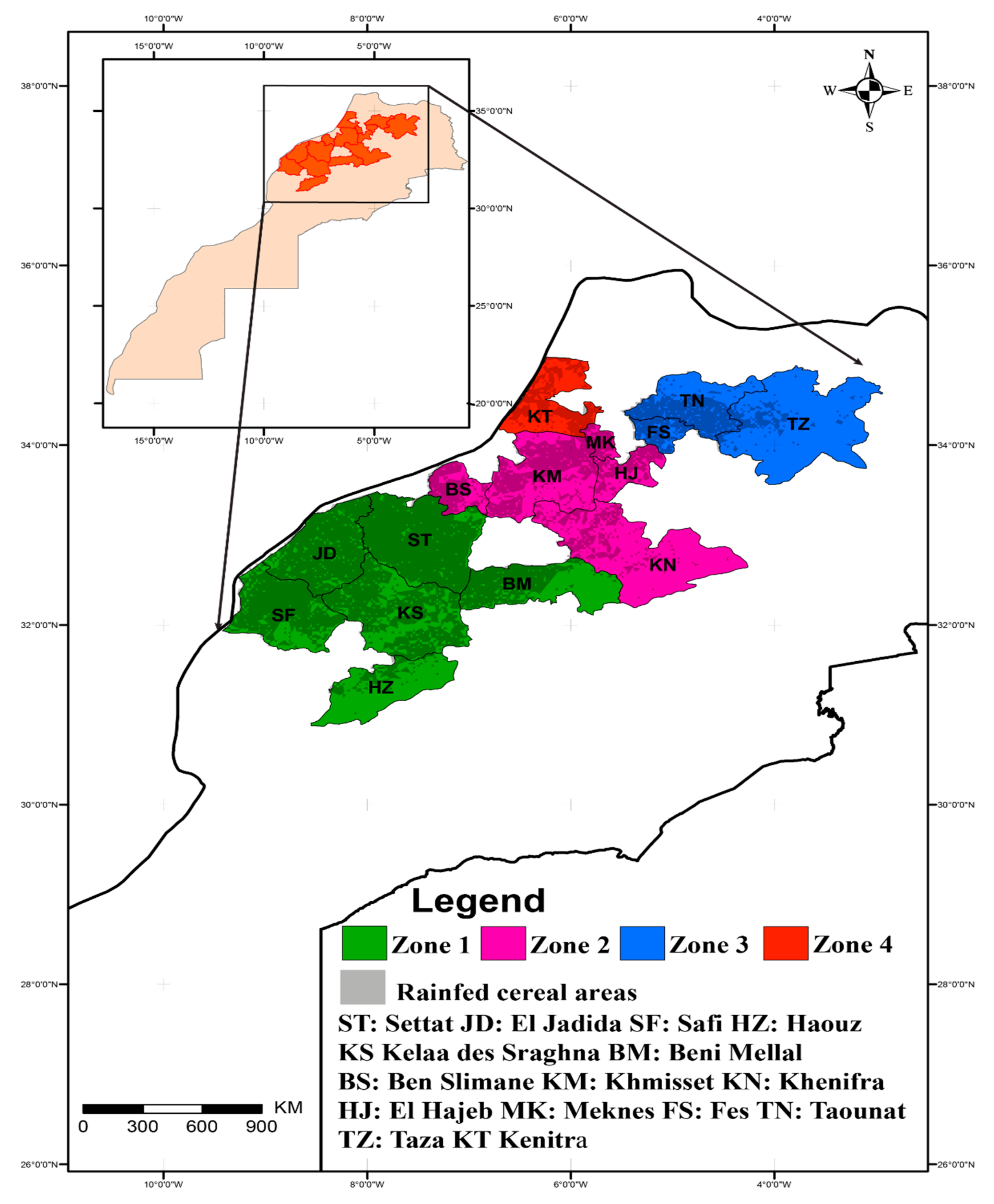
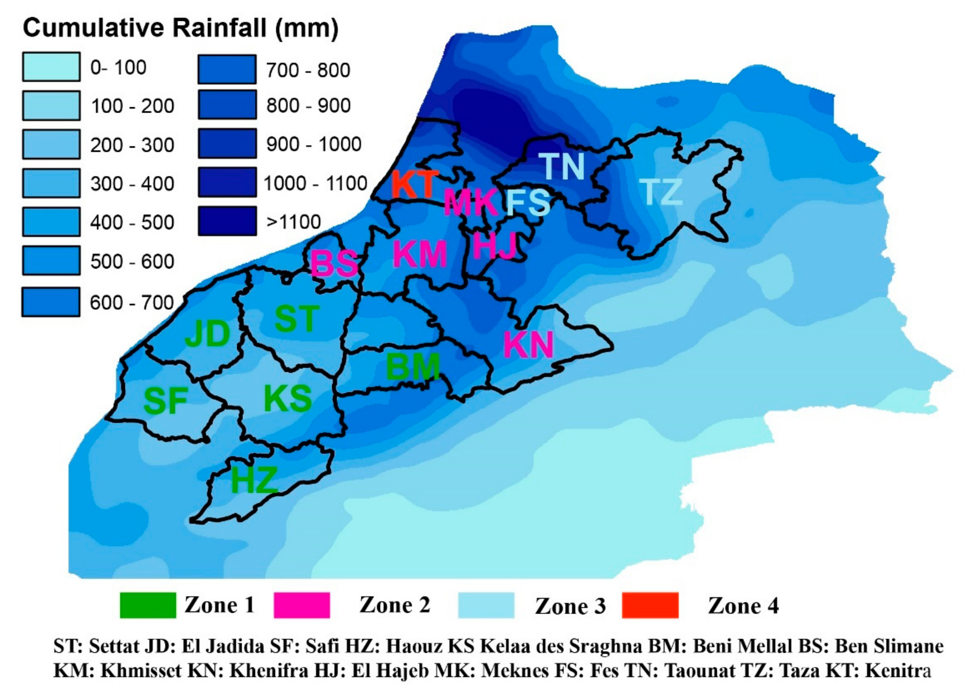
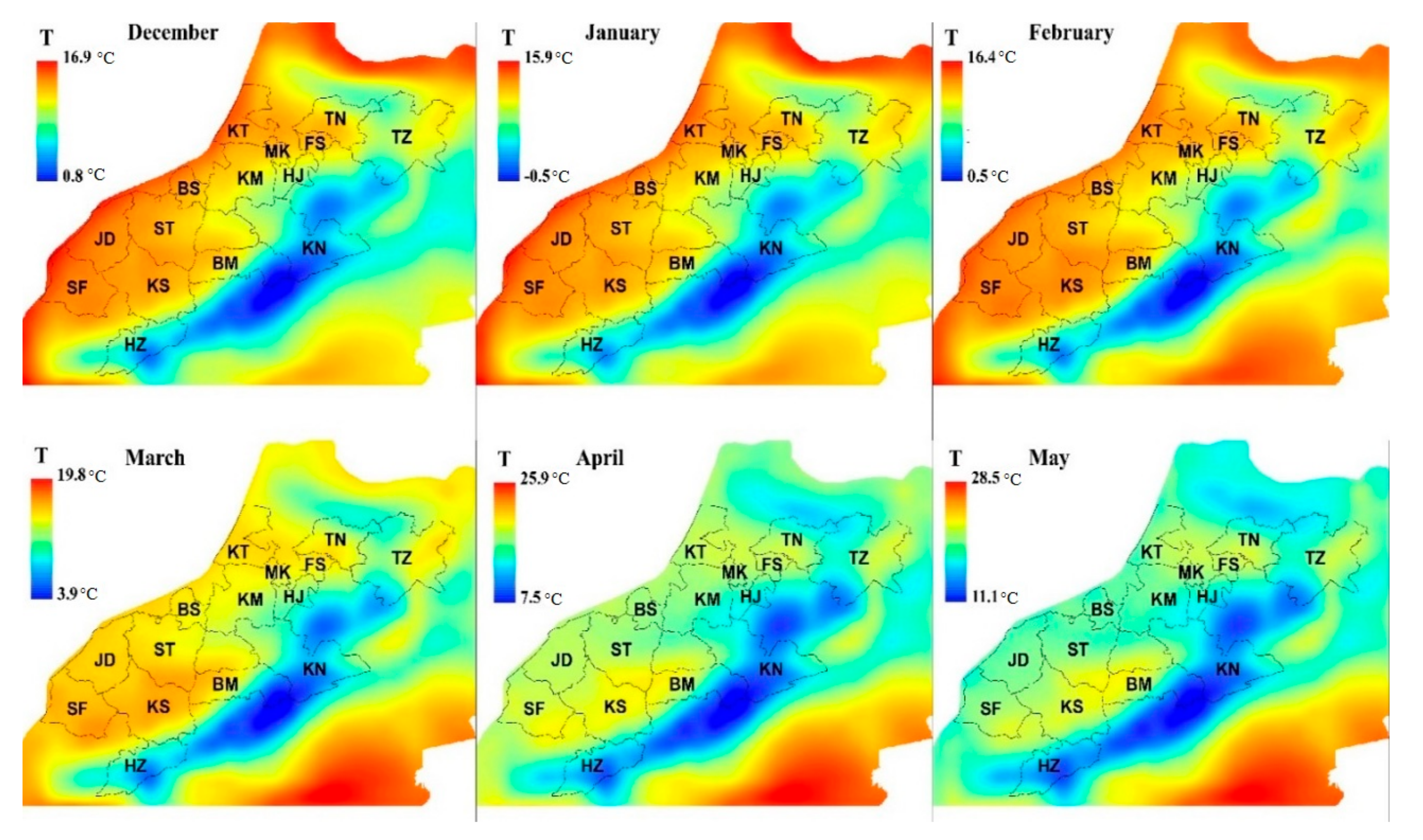
2.1. Study Area
2.2. Data
2.2.1. ERA5 Data and the SPEI
2.2.2. Yield Data
- -
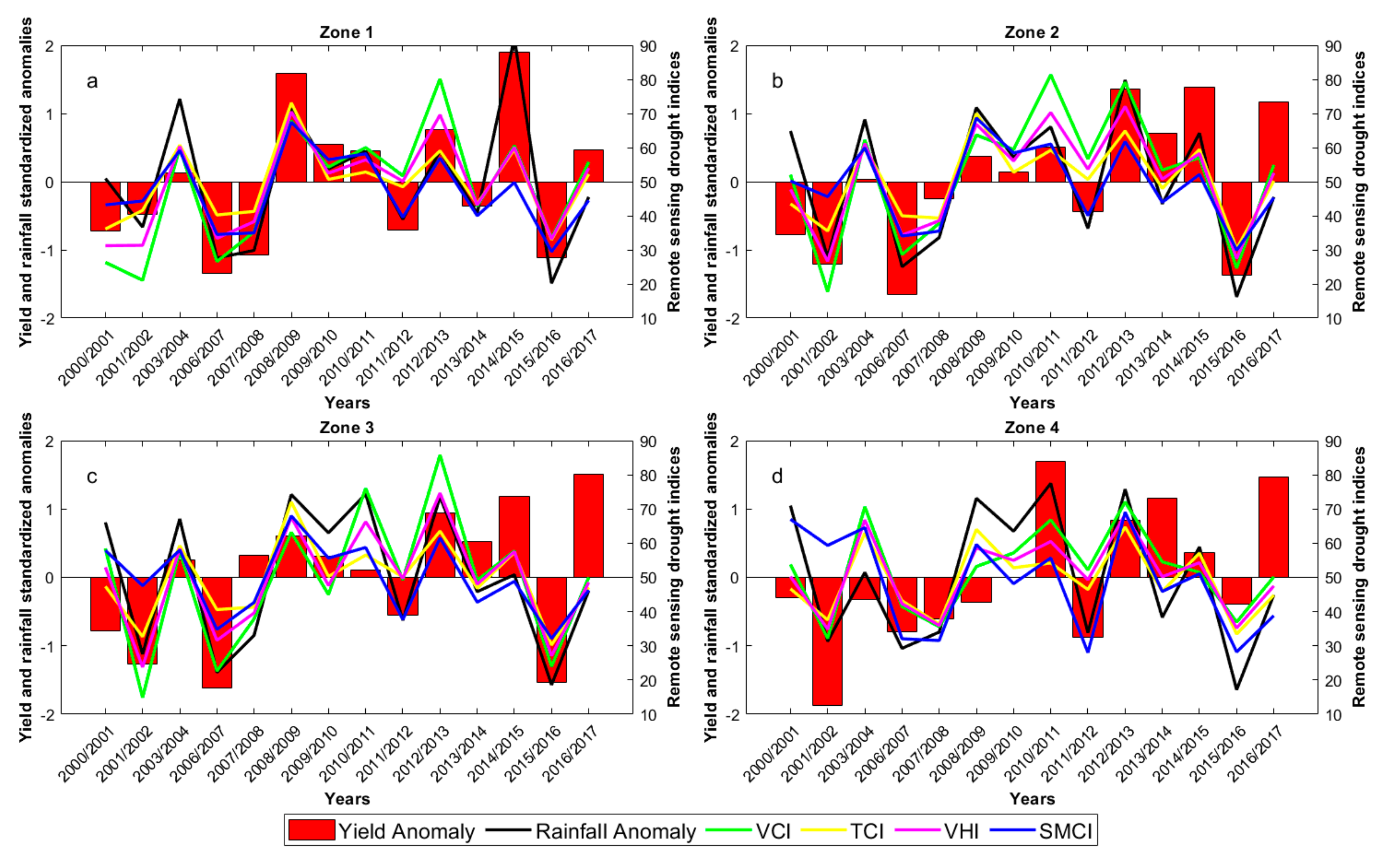
- The first group named “Zone 1” covers the southern province of the study area: Settat, El Jadida, Safi, Kelaa des Sraghnas, Haouz and Beni Mellal provinces. Because of the strong north-south rainfall gradient in Morocco, the group 1 area is characterized by low rainfall and high temperature and is consequently considered to be a less productive area. Please note that the Safi province receives a large amount of rainfall (355 mm from November to May on average over the study period using the ERA5 dataset) as it is located along the Atlantic Ocean. However, yields are low, which may be due to poor soils. In addition, a large rainfed area in the Beni Mellal province is located in the foothills of the Atlas Mountains, which has colder conditions than in the plains; yields are also quite low (1.5 t/ha on average over 2000–2017).
- -
- The second group named “Zone 2” covers the Ben Slimane, Khenifra, El Hajeb, Khemisset and Meknes provinces. They are located in the center of the study region with relatively high rainfall conditions (approximately 600 mm on average during the crop season), showing higher yields than those for group 1, with an average yield of approximately 1.9 t/ha.
- -
- The third group named “Zone 3” covers the provinces of Taza, Taounat, and Fes. Zone 3 is located north of Morocco, and it is characterized by higher rainfall compared with the other groups (approximately 680 mm). The average yield in this zone is approximately 1.5 t/ha.
- -
- The last group named “Zone 4” includes only the province of Kenitra. This province is located in the northeastern part of the country. Zone 4 is dominated by irrigated areas where cereals represent more than 60% of crops, including the Gharb plain. Although rainfed yields are only considered in this study, it is likely that any rainfed fields neighboring irrigated areas benefit from the supplementary water supply. The combined high rainfall amount and high coastal air moisture may justify the high yield observed in this province compared with the other zones.
2.2.3. Remote Sensing-Based Drought Indices
The Vegetation Condition Index (VCI)
The Temperature Condition Index (TCI)
The Vegetation Health Index (VHI)
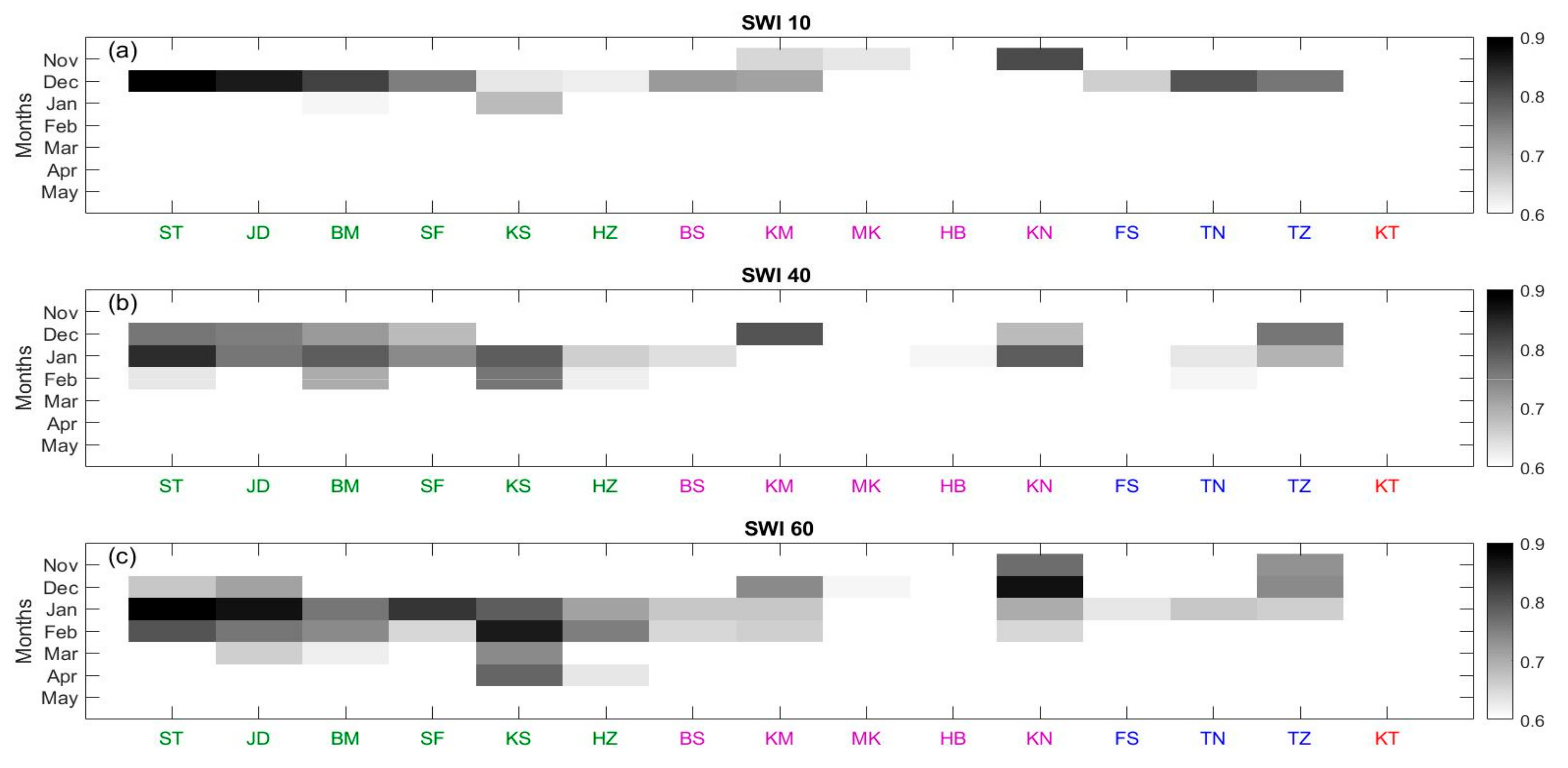
The Soil Water Index (SWI)
The Soil Moisture Condition Index (SMCI)
2.2.4. Land Data Assimilation System (LDAS) Outputs
2.3. Methods
2.3.1. Identification of Rainfed Cereal Areas
- (a)
- ECOCLIMAP-II land cover [113,114] developed by CNRM at a 1 km resolution (https://opensource.umr-cnrm.fr/projects/ecoclimap/wiki) was used to select the pixels corresponding to C3 crops, including both irrigated and rainfed fields.
- (b)
- The land cover map at a 300 m resolution provided by the Climate Change Initiative land cover project of the ESA (https://www.esa-landcover-cci.org/) was used to distinguish between irrigated and rainfed crops.
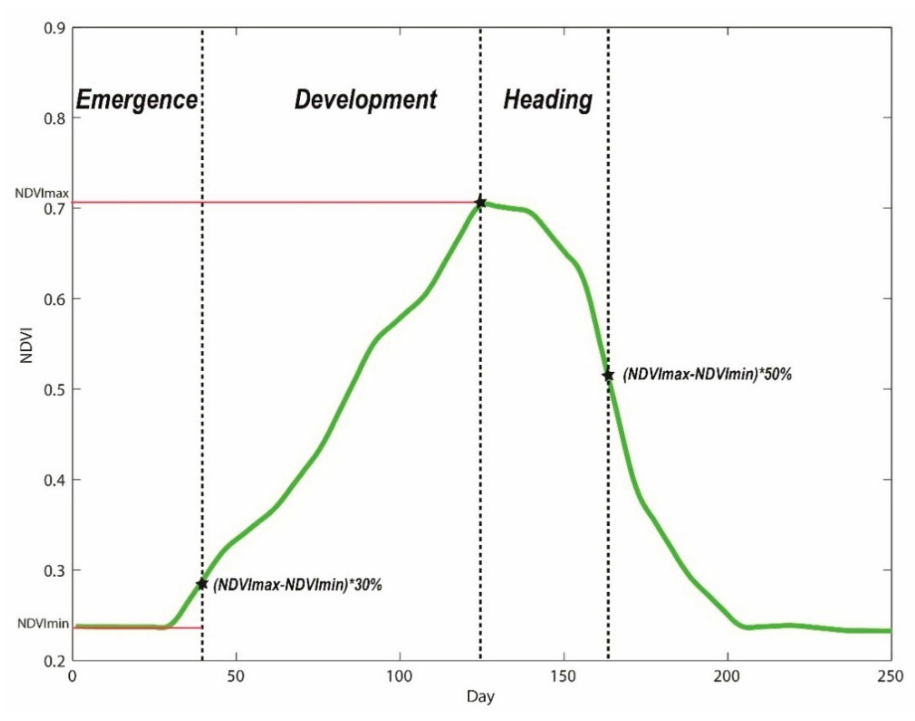
2.3.2. Identification of Major Phenological Stage
- Emergence stage: The emergence stage starts when the NDVI reaches 30% of the difference between NDVI max and NDVI min.
- Development stage: A drastic increase in the NDVI is observed at the start of the season. The development stage was defined as starting when the NDVI value reached 30% of the difference between the maximum and minimum of the NDVI values. The stage ends at the heading stage (see below).
- Heading stage: The heading stage starts when the NDVI reaches its maximum value and ends at the harvesting stage.
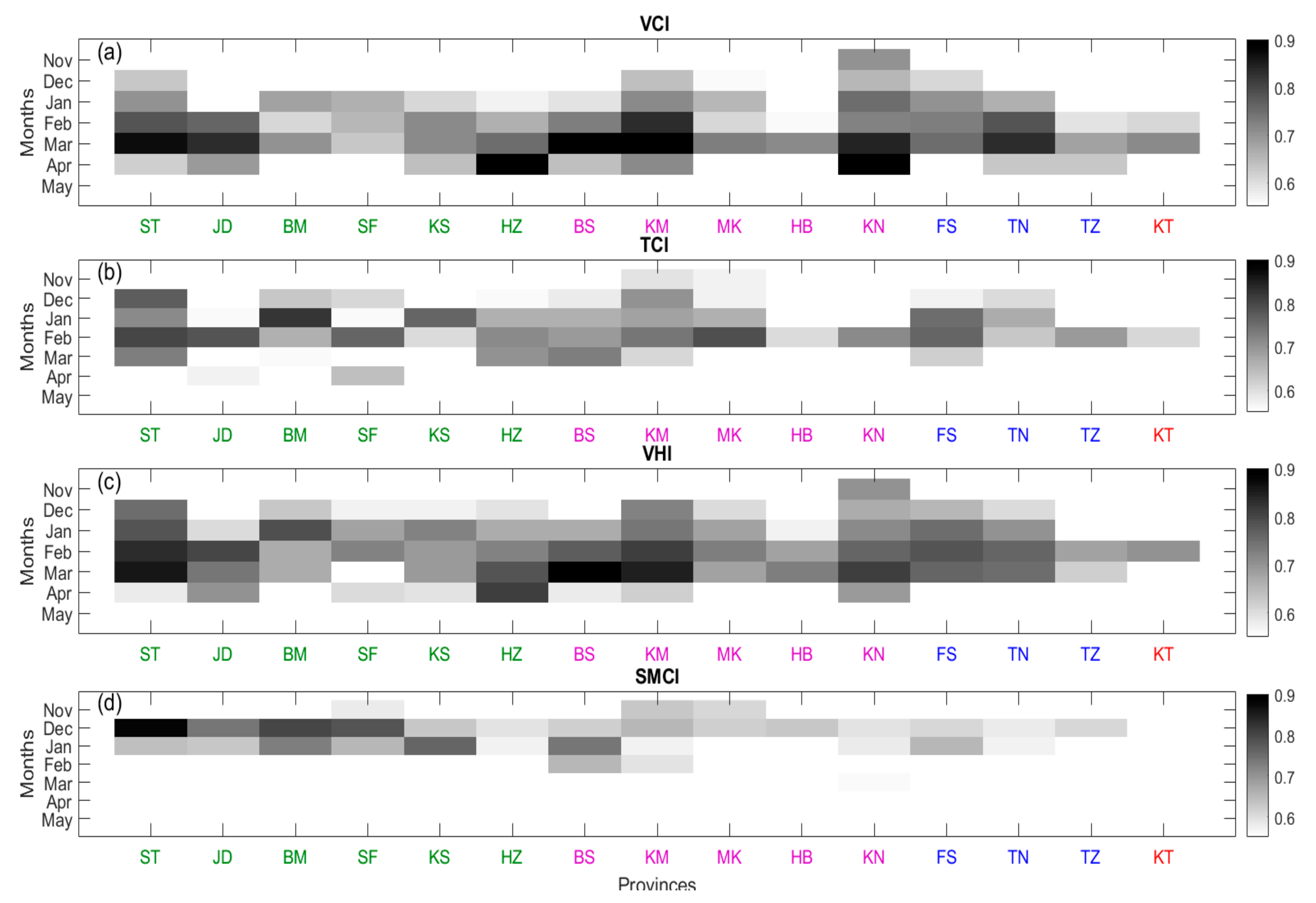
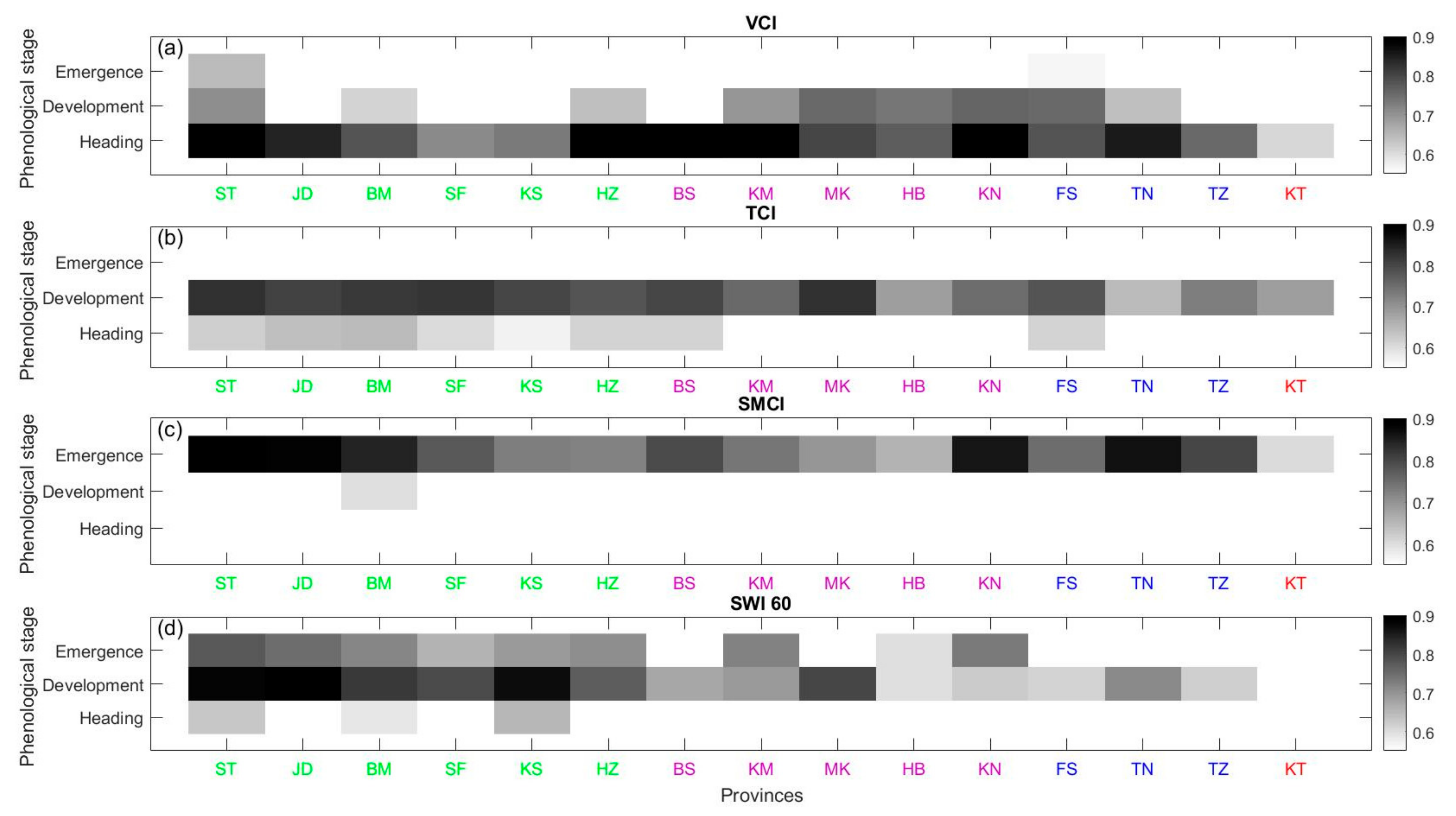
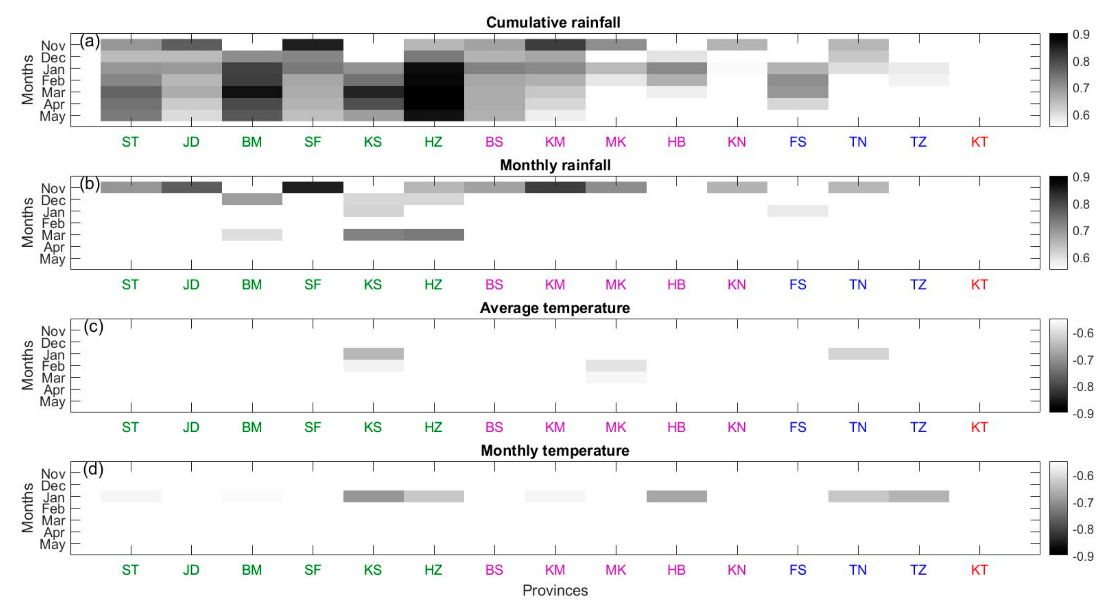
2.3.3. Correlation Analysis between Drought Indices and Rainfed Cereal Yield
3. Results
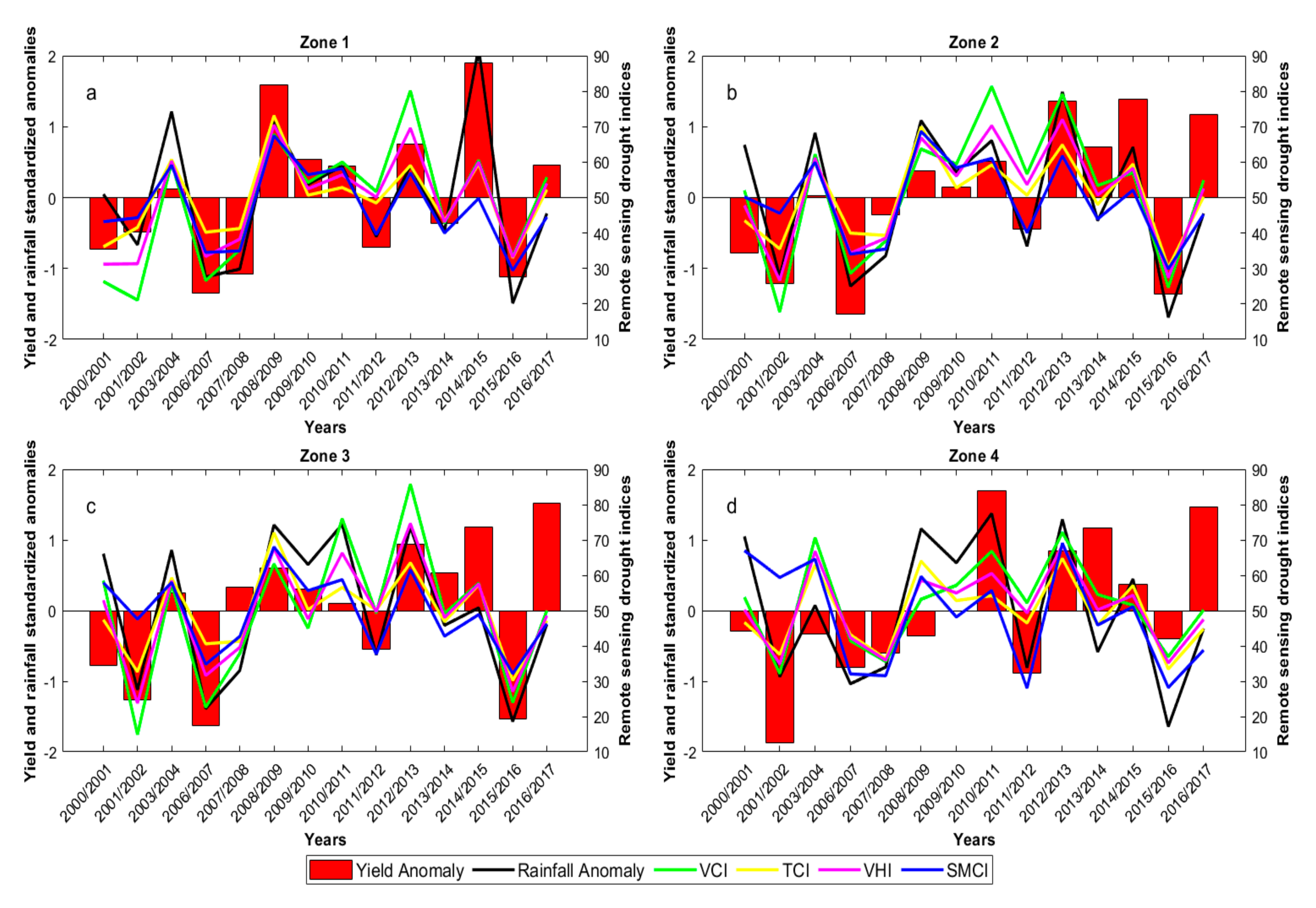
3.1. Satellite Drought Indices and Yield Time Series
3.1.1. Seasonal Scale
3.1.2. Monthly Scale
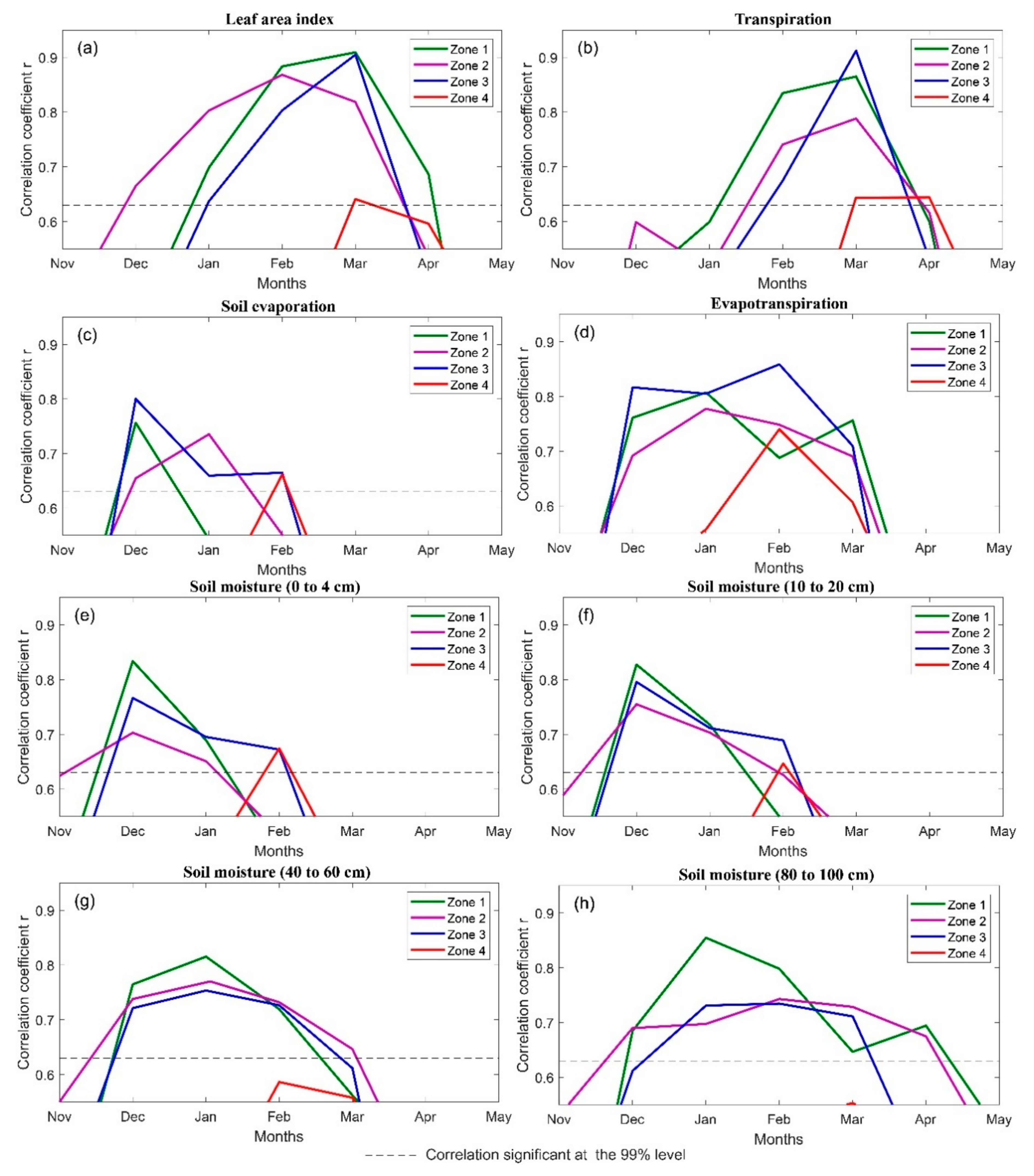
3.2. LDAS Outputs and Yields Time Series
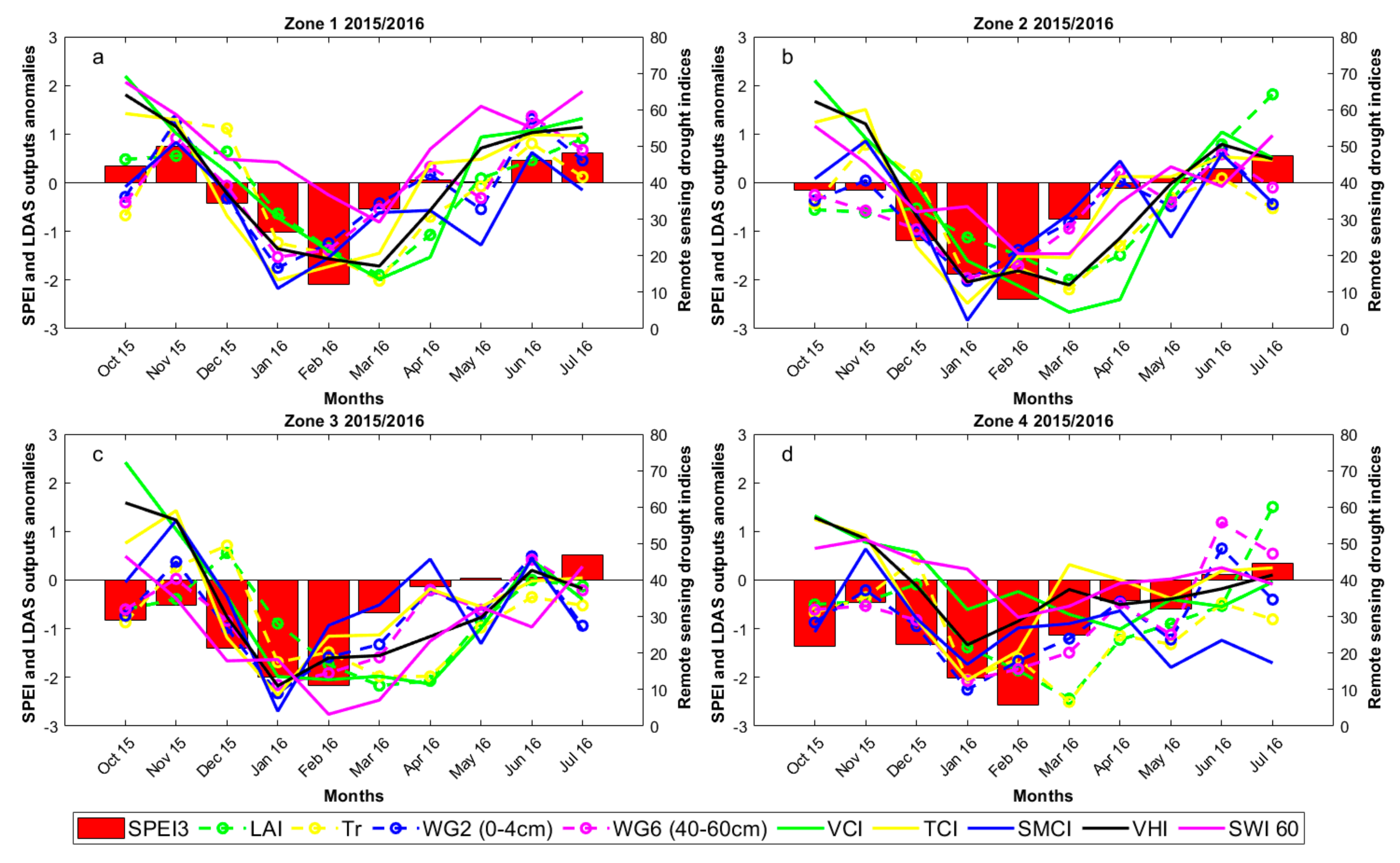
3.3. Case Study: 2015/2016
4. Discussion
4.1. The Added Value of an LDAS
4.2. Phenological Stages Versus Monthly Scale
4.3. Alpha Value for the Computation of VHI
5. Conclusions
Author Contributions
Funding
Acknowledgments
Conflicts of Interest
Appendix A


References
- Kumar, V. An early warning system for agricultural drought in an arid region using limited data. J. Arid Environ. 1998. [Google Scholar] [CrossRef]
- Páscoa, P.; Gouveia, C.M.; Russo, A.; Trigo, R.M. The role of drought on wheat yield interannual variability in the Iberian Peninsula from 1929 to 2012. Int. J. Biometeorol. 2017. [Google Scholar] [CrossRef]
- Ribeiro, A.F.S.; Russo, A.; Gouveia, C.M.; Páscoa, P. Modelling drought-related yield losses in Iberia using remote sensing and multiscalar indices. Theor. Appl. Climatol. 2019. [Google Scholar] [CrossRef]
- FAO. The Impact of of Natural Hazards and Disasters on Agriculture, Food Security and Nutrition; FAO: Rome, Italy, 2017; ISBN 978-92-5-130359-7. [Google Scholar]
- Schilling, J.; Freier, K.P.; Hertig, E.; Scheffran, J. Climate change, vulnerability and adaptation in North Africa with focus on Morocco. Agric. Ecosyst. Environ. 2012. [Google Scholar] [CrossRef]
- Schilling, J.; Hertig, E.; Tramblay, Y.; Scheffran, J. Climate change vulnerability, water resources and social implications in North Africa. Reg. Environ. Chang. 2020. [Google Scholar] [CrossRef]
- Tigkas, D.; Tsakiris, G. Early Estimation of Drought Impacts on Rainfed Wheat Yield in Mediterranean Climate. Environ. Process. 2015. [Google Scholar] [CrossRef]
- Karrou, M.; Oweis, T. Water and land productivities of wheat and food legumes with deficit supplemental irrigation in a Mediterranean environment. Agric. Water Manag. 2012. [Google Scholar] [CrossRef]
- Jarlan, L.; Abaoui, J.; Duchemin, B.; Ouldbba, A.; Tourre, Y.M.; Khabba, S.; Le Page, M.; Balaghi, R.; Mokssit, A.; Chehbouni, G. Linkages between common wheat yields and climate in Morocco (1982–2008). Int. J. Biometeorol. 2014, 58, 1489–1502. [Google Scholar] [CrossRef]
- Balaghi, R.; Tychon, B.; Eerens, H.; Jlibene, M. Empirical regression models using NDVI, rainfall and temperature data for the early prediction of wheat grain yields in Morocco. Int. J. Appl. Earth Obs. Geoinf. 2008. [Google Scholar] [CrossRef]
- Latiri, K.; Lhomme, J.P.; Annabi, M.; Setter, T.L. Wheat production in Tunisia: Progress, inter-annual variability and relation to rainfall. Eur. J. Agron. 2010, 33, 33–42. [Google Scholar] [CrossRef]
- Agoumi, A. Vulnerability of North African Countries to Climatic Changes; International Institute for Sustainable Development: Winnipeg, MB, Canada, 2003. [Google Scholar]
- Driouech, F.; Déqué, M.; Mokssit, A. Numerical simulation of the probability distribution function of precipitation over Morocco. Clim. Dyn. 2009. [Google Scholar] [CrossRef]
- IPCC. Managing the Risks of Extreme Events and Disasters to Advance Climate Change Adaptation. Available online: https://www.ipcc.ch/report/managing-the-risks-of-extreme-events-and-disasters-to-advance-climate-change-adaptation/ (accessed on 27 November 2020).
- Hertig, E.; Tramblay, Y. Regional downscaling of Mediterranean droughts under past and future climatic conditions. Glob. Planet. Chang. 2017. [Google Scholar] [CrossRef]
- Lehner, F.; Coats, S.; Stocker, T.F.; Pendergrass, A.G.; Sanderson, B.M.; Raible, C.C.; Smerdon, J.E. Projected drought risk in 1.5 °C and 2 °C warmer climates. Geophys. Res. Lett. 2017. [Google Scholar] [CrossRef]
- Dai, A. Drought under global warming: A review. Wiley Interdiscip. Rev. Clim. Chang. 2011. [Google Scholar] [CrossRef]
- Vogel, M.M.; Hauser, M.; Seneviratne, S.I. Projected changes in hot, dry and wet extreme events’ clusters in CMIP6 multi-model ensemble. Environ. Res. Lett. 2020. [Google Scholar] [CrossRef]
- Ministère de l’Agriculture, de la Pêche Maritime, Développement Rural et des eaux et Forêts, Agriculture en chiffre au Maroc. Available online: https://www.agriculture.gov.ma/pages/publications/agriculture-en-chiffres-2018-edition-2019 (accessed on 27 November 2020).
- Vicente-Serrano, S.; Cuadrat-Prats, J.M.; Romo, A. Early prediction of crop production using drought indices at different time-scales and remote sensing data: Application in the Ebro Valley (north-east Spain). Int. J. Remote Sens. 2006. [Google Scholar] [CrossRef]
- Wilhite, D.A.; Glantz, M.H. Water International Understanding: The Drought Phenomenon: The Role of Definitions Understanding: The Drought Phenomenon: The Role of Definitions. Water Int. 1985, 10, 111–120. [Google Scholar] [CrossRef]
- Ciais, P.; Reichstein, M.; Viovy, N.; Granier, A.; Ogée, J.; Allard, V.; Aubinet, M.; Buchmann, N.; Bernhofer, C.; Carrara, A.; et al. Europe-wide reduction in primary productivity caused by the heat and drought in 2003. Nature 2005. [Google Scholar] [CrossRef]
- Mishra, A.K.; Singh, V.P. A review of drought concepts. J. Hydrol. 2010. [Google Scholar] [CrossRef]
- Balaghi, R.; Jlibene, M.; Tychon, B.; Eerens, H. Agrometeorological Cereal Yield Forecasting in Morocco; Institut National de la Recherche Agronomique: Rabat, Morocco, 2013; ISBN 978-9954-0-6683-6. [Google Scholar]
- Ewert, F.; Rodriguez, D.; Jamieson, P.; Semenov, M.A.; Mitchell, R.A.C.; Goudriaan, J.; Porter, J.R.; Kimball, B.A.; Pinter, P.J.; Manderscheid, R.; et al. Effects of elevated CO2 and drought on wheat: Testing crop simulation models for different experimental and climatic conditions. Agric. Ecosyst. Environ. 2002, 93, 249–266. [Google Scholar] [CrossRef]
- Van Herwaarden, A.F.; Farquhar, G.D.; Angus, J.F.; Richards, R.A.; Howe, G.N. “Haying-off”, the negative grain yield response of dryland wheat to nitrogen fertiliser. I. Biomass, grain yield, and water use. Aust. J. Agric. Res. 1998, 49, 1067. [Google Scholar] [CrossRef]
- McKee, T.B.; Nolan, J.; Kleist, J. The relationship of drought frequency and duration to time scales. Prepr. Eighth Conf. Appl. Climatol. Am. Meteor Soc. 1993, 17, 179–184. [Google Scholar]
- Kazmi, D.H.; Rasul, G. Agrometeorological wheat yield prediction in rainfed Potohar region of Pakistan. Agric. Sci. 2012. [Google Scholar] [CrossRef]
- Salman, A.Z.; Al-Karablieh, E.K. An early warning system for wheat production in low rainfall areas of Jordan. J. Arid Environ. 2001. [Google Scholar] [CrossRef]
- Kumar, V.; Panu, U. Predictive assessment of severity of agricultural droughts based on agro-climatic factors. J. Am. Water Resour. Assoc. 1997. [Google Scholar] [CrossRef]
- Heng, L.K.; Asseng, S.; Mejahed, K.; Rusan, M. Optimizing wheat productivity in two rain-fed environments of the West Asia-North Africa region using a simulation model. Eur. J. Agron. 2007, 26, 121–129. [Google Scholar] [CrossRef]
- Timmermans, B.G.H.; Vos, J.; van Nieuwburg, J.; Stomph, T.J.; van der Putten, P.E.L. Germination rates of Solanum sisymbriffolium: Temperature response models, effects of temperature fluctuations and soil water potential. Seed Sci. Res. 2007, 17, 221–231. [Google Scholar] [CrossRef]
- Vicente-Serrano, S.M.; Beguería, S.; López-Moreno, J.I. A multiscalar drought index sensitive to global warming: The standardized precipitation evapotranspiration index. J. Clim. 2010. [Google Scholar] [CrossRef]
- Bijaber, N.; El Hadani, D.; Saidi, M.; Svoboda, M.D.; Wardlow, B.D.; Hain, C.R.; Poulsen, C.C.; Yessef, M.; Rochdi, A. Developing a remotely sensed drought monitoring indicator for Morocco. Geosciences 2018, 8, 55. [Google Scholar] [CrossRef]
- Hayes, M.J.; Svoboda, M.D.; Wardlow, B.D.; Anderson, M.C.; Kogan, F. Drought Monitoring: Historical and Current Perspectives. Available online: https://digitalcommons.unl.edu/droughtfacpub/94/ (accessed on 27 November 2020).
- Le Page, M.; Zribi, M. Analysis and Predictability of Drought In Northwest Africa Using Optical and Microwave Satellite Remote Sensing Products. Sci. Rep. 2019. [Google Scholar] [CrossRef]
- Zargar, A.; Sadiq, R.; Naser, B.; Khan, F.I. A review of drought indices. Environ. Rev. 2011, 19, 333–349. [Google Scholar] [CrossRef]
- Hazaymeh, K.; Hassan, Q.K. Remote sensing of agricultural drought monitoring: A state of art review. AIMS Environ. Sci. 2016. [Google Scholar] [CrossRef]
- Singh, R.P.; Roy, S.; Kogan, F. Vegetation and temperature condition indices from NOAA AVHRR data for drought monitoring over India. Int. J. Remote Sens. 2003. [Google Scholar] [CrossRef]
- Liu, W.T.; Kogan, F.N. Monitoring regional drought using the vegetation condition index. Int. J. Remote Sens. 1996. [Google Scholar] [CrossRef]
- Unganai, L.S.; Kogan, F.N. Drought monitoring and corn yield estimation in southern Africa from AVHRR data. Remote Sens. Environ. 1998. [Google Scholar] [CrossRef]
- Salazar, L.; Kogan, F.; Roytman, L. Use of remote sensing data for estimation of winter wheat yield in the United States. Int. J. Remote Sens. 2007. [Google Scholar] [CrossRef]
- Vicente-Serrano, S.M. Evaluating the impact of drought using remote sensing in a Mediterranean, Semi-arid Region. Nat. Hazards 2007. [Google Scholar] [CrossRef]
- Kogan, F.N. Global Drought Watch from Space. Bull. Am. Meteorol. Soc. 1997. [Google Scholar] [CrossRef]
- Bento, V.A.; Trigo, I.F.; Gouveia, C.M.; DaCamara, C.C. Contribution of Land Surface Temperature (TCI) to Vegetation Health Index: A comparative study using clear sky and all-weather climate data records. Remote Sens. 2018, 9, 1324. [Google Scholar] [CrossRef]
- Bento, V.A.; Gouveia, C.M.; DaCamara, C.C.; Trigo, I.F. A climatological assessment of drought impact on vegetation health index. Agric. For. Meteorol. 2018. [Google Scholar] [CrossRef]
- Bento, V.A.; Gouveia, C.M.; DaCamara, C.C.; Libonati, R.; Trigo, I.F. The roles of NDVI and Land Surface Temperature when using the Vegetation Health Index over dry regions. Glob. Planet. Chang. 2020, 190, 103198. [Google Scholar] [CrossRef]
- Zhang, A.; Jia, G. Monitoring meteorological drought in semiarid regions using multi-sensor microwave remote sensing data. Remote Sens. Environ. 2013, 134, 12–23. [Google Scholar] [CrossRef]
- Reichle, R.H.; Koster, R.D.; Liu, P.; Mahanama, S.P.P.; Njoku, E.G.; Owe, M. Comparison and assimilation of global soil moisture retrievals from the Advanced Microwave Scanning Radiometer for the Earth Observing System (AMSR-E) and the Scanning Multichannel Microwave Radiometer (SMMR). J. Geophys. Res. 2007, 112, 1–14. [Google Scholar] [CrossRef]
- Albergel, C.; Munier, S.; Jennifer Leroux, D.; Dewaele, H.; Fairbairn, D.; Lavinia Barbu, A.; Gelati, E.; Dorigo, W.; Faroux, S.; Meurey, C.; et al. Sequential assimilation of satellite-derived vegetation and soil moisture products using SURFEX-v8.0: LDAS-Monde assessment over the Euro-Mediterranean area. Geosci. Model Dev. 2017. [Google Scholar] [CrossRef]
- Kumar, S.V.; Jasinski, M.; Mocko, D.M.; Rodell, M.; Borak, J.; Li, B.; Beaudoing, H.K.; Peters-Lidard, C.D. NCA-LDAS Land Analysis: Development and Performance of a Multisensor, Multivariate Land Data Assimilation System for the National Climate Assessment. J. Hydrometeorol. 2019. [Google Scholar] [CrossRef]
- Sawada, Y.; Koike, T.; Walker, J.P. A land data assimilation system for simultaneous simulation of soil moisture and vegetation dynamics. J. Geophys. Res. 2015. [Google Scholar] [CrossRef]
- McNally, A.; Arsenault, K.; Kumar, S.; Shukla, S.; Peterson, P.; Wang, S.; Funk, C.; Peters-Lidard, C.D.; Verdin, J.P. A land data assimilation system for sub-Saharan Africa food and water security applications. Sci. Data 2017. [Google Scholar] [CrossRef]
- Han, E.; Crow, W.T.; Holmes, T.; Bolten, J. Benchmarking a soil moisture data assimilation system for agricultural drought monitoring. J. Hydrometeorol. 2014, 15, 1117–1134. [Google Scholar] [CrossRef]
- Blyverket, J.; Hamer, P.D.; Schneider, P.; Albergel, C.; Lahoz, W.A. Monitoring soil moisture drought over northern high latitudes from space. Remote Sens. 2019, 10, 1200. [Google Scholar] [CrossRef]
- Bolten, J.D.; Crow, W.T.; Jackson, T.J.; Zhan, X.; Reynolds, C.A. Evaluating the Utility of Remotely Sensed Soil Moisture Retrievals for Operational Agricultural Drought Monitoring. IEEE J. Sel. Top. Appl. Earth Obs. Remote Sens. 2010. [Google Scholar] [CrossRef]
- Renzullo, L.J.; van Dijk, A.I.J.M.; Perraud, J.M.; Collins, D.; Henderson, B.; Jin, H.; Smith, A.B.; McJannet, D.L. Continental satellite soil moisture data assimilation improves root-zone moisture analysis for water resources assessment. J. Hydrol. 2014. [Google Scholar] [CrossRef]
- Draper, C.S.; Mahfouf, J.F.; Walker, J.P. An EKF assimilation of AMSR-E soil moisture into the ISBA land surface scheme. J. Geophys. Res. Atmos. 2009. [Google Scholar] [CrossRef]
- Albergel, C.; Calvet, J.C.; Mahfouf, J.F.; Rüdiger, C.; Barbu, A.L.; Lafont, S.; Roujean, J.L.; Walker, J.P.; Crapeau, M.; Wigneron, J.P. Monitoring of water and carbon fluxes using a land data assimilation system: A case study for southwestern France. Hydrol. Earth Syst. Sci. 2010. [Google Scholar] [CrossRef]
- Ragab, R. Towards a continuous operational system to estimate the root-zone soil moisture from intermittent remotely sensed surface moisture. J. Hydrol. 1995. [Google Scholar] [CrossRef]
- Walker, J.P.; Willgoose, G.R.; Kalma, J.D. One-dimensional soil moisture profile retrieval by assimilation of near-surface measurements: A simplified soil moisture model and field application. J. Hydrometeorol. 2001. [Google Scholar] [CrossRef]
- Bolten, J.D.; Crow, W.T. Improved prediction of quasi-global vegetation conditions using remotely-sensed surface soil moisture. Geophys. Res. Lett. 2012. [Google Scholar] [CrossRef]
- Albergel, C.; Munier, S.; Bocher, A.; Bonan, B.; Zheng, Y.; Draper, C.; Leroux, D.J.; Calvet, J.C. LDAS-Monde sequential assimilation of satellite derived observations applied to the contiguous US: An ERA-5 driven reanalysis of the land surface variables. Remote Sens. 2018, 10, 1627. [Google Scholar] [CrossRef]
- Kogan, F.N. Application of vegetation index and brightness temperature for drought detection. Adv. Sp. Res. 1995. [Google Scholar] [CrossRef]
- Gao, B.C. NDWI—A normalized difference water index for remote sensing of vegetation liquid water from space. Remote Sens. Environ. 1996. [Google Scholar] [CrossRef]
- Wang, P.X.; Li, X.W.; Gong, J.Y.; Song, C. Vegetation temperature condition index and its application for drought monitoring. In Proceedings of the International Geoscience and Remote Sensing Symposium (IGARSS), Sydney, Ausralia, 9–13 July 2001. [Google Scholar]
- Peters, A.J.; Walter-Shea, E.A.; Ji, L.; Viña, A.; Hayes, M.; Svoboda, M.D. Drought monitoring with NDVI-based Standardized Vegetation Index. Photogramm. Eng. Remote Sens. 2002, 68, 71–75. [Google Scholar]
- Gu, Y.; Brown, J.F.; Verdin, J.P.; Wardlow, B. A five-year analysis of MODIS NDVI and NDWI for grassland drought assessment over the central Great Plains of the United States. Geophys. Res. Lett. 2007. [Google Scholar] [CrossRef]
- Wang, L.; Qu, J.J. NMDI: A normalized multi-band drought index for monitoring soil and vegetation moisture with satellite remote sensing. Geophys. Res. Lett. 2007. [Google Scholar] [CrossRef]
- Ghulam, A.; Li, Z.L.; Qin, Q.; Yimit, H.; Wang, J. Estimating crop water stress with ETM+ NIR and SWIR data. Agric. For. Meteorol. 2008. [Google Scholar] [CrossRef]
- Rhee, J.; Im, J.; Carbone, G.J. Monitoring agricultural drought for arid and humid regions using multi-sensor remote sensing data. Remote Sens. Environ. 2010, 114, 2875–2887. [Google Scholar] [CrossRef]
- Anderson, M.C.; Zolin, C.A.; Sentelhas, P.C.; Hain, C.R.; Semmens, K.; Tugrul Yilmaz, M.; Gao, F.; Otkin, J.A.; Tetrault, R. The Evaporative Stress Index as an indicator of agricultural drought in Brazil: An assessment based on crop yield impacts. Remote Sens. Environ. 2016, 174, 82–99. [Google Scholar] [CrossRef]
- Zhang, X.; Chen, N.; Li, J.; Chen, Z.; Niyogi, D. Multi-sensor integrated framework and index for agricultural drought monitoring. Remote Sens. Environ. 2017, 188, 141–163. [Google Scholar] [CrossRef]
- Jiao, W.; Tian, C.; Chang, Q.; Novick, K.A.; Wang, L. Agricultural and Forest Meteorology A new multi-sensor integrated index for drought monitoring. Agric. For. Meteorol. 2019, 268, 74–85. [Google Scholar] [CrossRef]
- Hu, T.; Renzullo, L.J.; van Dijk, A.I.J.M.; He, J.; Tian, S.; Xu, Z.; Zhou, J.; Liu, T.; Liu, Q. Monitoring agricultural drought in Australia using MTSAT-2 land surface temperature retrievals. Remote Sens. Environ. 2020, 236. [Google Scholar] [CrossRef]
- Driouech, F.; Déqué, M.; Sánchez-Gómez, E. Weather regimes-Moroccan precipitation link in a regional climate change simulation. Glob. Planet. Chang. 2010, 72, 1–10. [Google Scholar] [CrossRef]
- Knippertz, P.; Christoph, M.; Speth, P. Long-term precipitation variability in Morocco and the link to the large-scale circulation in recent and future climates. Meteorol. Atmos. Phys. 2003. [Google Scholar] [CrossRef]
- Balaghi, R.; Jlibene, M.; Tychon, B.; Mrabet, R. Gestion du risque de sécheresse agricole au Maroc. Sci. Chang. Planét. Sécheresse 2007, 18, 169–176. [Google Scholar] [CrossRef]
- Beguería, S.; Vicente-Serrano, S.M.; Reig, F.; Latorre, B. Standardized precipitation evapotranspiration index (SPEI) revisited: Parameter fitting, evapotranspiration models, tools, datasets and drought monitoring. Int. J. Climatol. 2014. [Google Scholar] [CrossRef]
- Abbasi, A.; Khalili, K.; Behmanesh, J.; Shirzad, A. Drought monitoring and prediction using SPEI index and gene expression programming model in the west of Urmia Lake. Theor. Appl. Climatol. 2019, 138, 553–567. [Google Scholar] [CrossRef]
- Tirivarombo, S.; Osupile, D.; Eliasson, P. Drought monitoring and analysis: Standardised Precipitation Evapotranspiration Index (SPEI) and Standardised Precipitation Index (SPI). Phys. Chem. Earth 2018, 106, 1–10. [Google Scholar] [CrossRef]
- Wang, F.; Yang, H.; Wang, Z.; Zhang, Z.; Li, Z. Drought evaluation with CMORPH satellite precipitation data in the Yellow River basin by using Gridded Standardized Precipitation Evapotranspiration Index. Remote Sens. 2019, 11, 485. [Google Scholar] [CrossRef]
- Hersbach, H.; Bell, B.; Berrisford, P.; Hirahara, S.; Horányi, A.; Muñoz-Sabater, J.; Nicolas, J.; Peubey, C.; Radu, R.; Schepers, D.; et al. The ERA5 global reanalysis. Q. J. R. Meteorol. Soc. 2020. [Google Scholar] [CrossRef]
- Begueria, S.; Serrano, V.; Sawasawa, H. SPEI: Calculation of Standardised Precipitation-Evapotranspiration Index. R Package Version 1.7. Available online: https://cran.r-project.org/web/packages/SPEI/SPEI.pdf (accessed on 27 November 2020).
- Allen, R.G.; Pereira, L.S.; Raes, D.; Smith, M. Crop Evapotranspiration—Guidelines for Computing Crop Water Requirements—FAO Irrigation and Drainage Paper 56. Available online: https://appgeodb.nancy.inra.fr/biljou/pdf/Allen_FAO1998.pdf (accessed on 27 November 2020).
- Jlibene, M. Options Génétiques D’adaptation du Blé Tendre au Changement Climatique. Prix Hassan II pour L’innovation et la Recherche, Édition 2009. Available online: https://www.inra.org.ma/sites/default/files/publications/ouvrages/jlibene11.pdf (accessed on 27 November 2020).
- Bouras, E.; Jarlan, L.; Khabba, S.; Er-Raki, S.; Dezetter, A.; Sghir, F.; Tramblay, Y. Assessing the impact of global climate changes on irrigated wheat yields and water requirements in a semi-arid environment of Morocco. Sci. Rep. 2019, 9. [Google Scholar] [CrossRef]
- Ryan, J.; Monem, M.A.; Amri, A. Nitrogen fertilizer response of some barley varieties in semi-arid conditions in Morocco. J. Agric. Sci. Technol. 2009, 11, 227–236. [Google Scholar]
- Duchemin, B.; Fieuzal, R.; Rivera, M.; Ezzahar, J.; Jarlan, L.; Rodriguez, J.; Hagolle, O.; Watts, C. Impact of Sowing Date on Yield and Water Use Efficiency of Wheat Analyzed through Spatial Modeling and FORMOSAT-2 Images. Remote Sens. 2015, 7, 5951–5979. [Google Scholar] [CrossRef]
- Kaufman, L.; Rousseeuw, P.J. Finding Groups in Data: An Introduction to Cluster Analysis (Wiley Series in Probability and Statistics). Available online: https://www.wiley.com/en-us/Finding+Groups+in+Data%3A+An+Introduction+to+Cluster+Analysis-p-9780470317488 (accessed on 27 November 2020).
- Du, L.; Tian, Q.; Yu, T.; Meng, Q.; Jancso, T.; Udvardy, P.; Huang, Y. A comprehensive drought monitoring method integrating MODIS and TRMM data. Int. J. Appl. Earth Obs. Geoinf. 2013. [Google Scholar] [CrossRef]
- Kogan, F.N. Droughts of the late 1980s in the United States as derived from NOAA polar-orbiting satellite data. Bull. Am. Meteorol. Soc. 1995. [Google Scholar] [CrossRef]
- Holben, B.N. Characteristics of maximum-value composite images from temporal AVHRR data. Int. J. Remote Sens. 1986. [Google Scholar] [CrossRef]
- Wan, Z. A generalized split-window algorithm for retrieving land-surface temperature from space. IEEE Trans. Geosci. Remote Sens. 1996. [Google Scholar] [CrossRef]
- Qiu, J.; Crow, W.T.; Nearing, G.S.; Mo, X.; Liu, S. The impact of vertical measurement depth on the information content of soil moisture times series data. Geophys. Res. Lett. 2014. [Google Scholar] [CrossRef]
- Ceballos, A.; Scipal, K.; Wagner, W.; Martínez-Fernández, J. Validation of ERS scatterometer-derived soil moisture data in the central part of the Duero Basin, Spain. Hydrol. Process. 2005. [Google Scholar] [CrossRef]
- Albergel, C.; Rüdiger, C.; Pellarin, T.; Calvet, J.C.; Fritz, N.; Froissard, F.; Suquia, D.; Petitpa, A.; Piguet, B.; Martin, E. From near-surface to root-zone soil moisture using an exponential filter: An assessment of the method based on in-situ observations and model simulations. Hydrol. Earth Syst. Sci. 2008. [Google Scholar] [CrossRef]
- Brocca, L.; Hasenauer, S.; Lacava, T.; Melone, F.; Moramarco, T.; Wagner, W.; Dorigo, W.; Matgen, P.; Martínez-Fernández, J.; Llorens, P.; et al. Soil moisture estimation through ASCAT and AMSR-E sensors: An intercomparison and validation study across Europe. Remote Sens. Environ. 2011. [Google Scholar] [CrossRef]
- Zribi, M.; Paris Anguela, T.; Duchemin, B.; Lili, Z.; Wagner, W.; Hasenauer, S.; Chehbouni, A. Relationship between soil moisture and vegetation in the Kairouan plain region of Tunisia using low spatial resolution satellite data. Water Resour. Res. 2010. [Google Scholar] [CrossRef]
- Wagner, W.; Lemoine, G.; Rott, H. A method for estimating soil moisture from ERS Scatterometer and soil data. Remote Sens. Environ. 1999. [Google Scholar] [CrossRef]
- Bauer-Marschallinger, B. Copernicus Global Land Operations “Vegetation and Energy”. Copernicus Publ. Prod. User Man. 2018, 51, 1–85. [Google Scholar]
- Paulik, C.; Dorigo, W.; Wagner, W.; Kidd, R. Validation of the ASCAT soil water index using in situ data from the International Soil moisture network. Int. J. Appl. Earth Obs. Geoinf. 2014, 30, 1–8. [Google Scholar] [CrossRef]
- Bartalis, Z.; Naeimi, V.; Wagner, W. ASCAT Soil Moisture Product Handbook; ASCAT Soil Moisture Report Series, No. 15; Institute of Photogrammetry and Remote Sensing, Vienna University of Technology: Vienna, Austria, 2008. [Google Scholar]
- Krueger, E.S.; Ochsner, T.E.; Quiring, S.M. Development and evaluation of soil moisture-based indices for agricultural drought monitoring. Agron. J. 2019, 111, 1392–1406. [Google Scholar] [CrossRef]
- Dorigo, W.; Wagner, W.; Albergel, C.; Albrecht, F.; Balsamo, G.; Brocca, L.; Chung, D.; Ertl, M.; Forkel, M.; Gruber, A.; et al. ESA CCI Soil Moisture for improved Earth system understanding: State-of-the art and future directions. Remote Sens. Environ. 2017, 203, 185–215. [Google Scholar] [CrossRef]
- Masson, V.; Le Moigne, P.; Martin, E.; Faroux, S.; Alias, A.; Alkama, R.; Belamari, S.; Barbu, A.; Boone, A.; Bouyssel, F.; et al. The SURFEXv7.2 land and ocean surface platform for coupled or offline simulation of earth surface variables and fluxes. Geosci. Model Dev. 2013. [Google Scholar] [CrossRef]
- Fairbairn, D.; Lavinia Barbu, A.; Napoly, A.; Albergel, C.; Mahfouf, J.F.; Calvet, J.C. The effect of satellite-derived surface soil moisture and leaf area index land data assimilation on streamflow simulations over France. Hydrol. Earth Syst. Sci. 2017. [Google Scholar] [CrossRef]
- Mahfouf, J.F.; Bergaoui, K.; Draper, C.; Bouyssel, F.; Taillefer, F.; Taseva, L. A comparison of two off-line soil analysis schemes for assimilation of screen level observations. J. Geophys. Res. Atmos. 2009. [Google Scholar] [CrossRef]
- Noilhan, J.; Mahfouf, J.F. The ISBA land surface parameterisation scheme. Glob. Planet. Chang. 1996. [Google Scholar] [CrossRef]
- Calvet, J.C.; Noilhan, J.; Roujean, J.L.; Bessemoulin, P.; Cabelguenne, M.; Olioso, A.; Wigneron, J.P. An interactive vegetation SVAT model tested against data from six contrasting sites. Agric. For. Meteorol. 1998. [Google Scholar] [CrossRef]
- Gibelin, A.L.; Calvet, J.C.; Roujean, J.L.; Jarlan, L.; Los, S.O. Ability of the land surface model ISBA-A-gs to simulate leaf area index at the global scale: Comparison with satellites products. J. Geophys. Res. Atmos. 2006. [Google Scholar] [CrossRef]
- Genovese, G.; Vignolles, C.; Nègre, T.; Passera, G. A methodology for a combined use of normalised difference vegetation index and CORINE land cover data for crop yield monitoring and forecasting. A case study on Spain. Agronomie 2001. [Google Scholar] [CrossRef]
- Faroux, S.; Kaptué Tchuenté, A.T.; Roujean, J.-L.; Masson, V.; Martin, E.; Le Moigne, P. ECOCLIMAP-II/Europe: A twofold database of ecosystems and surface parameters at 1 km resolution based on satellite information for use in land surface, meteorological and climate models. Geosci. Model Dev. 2013. [Google Scholar] [CrossRef]
- Masson, V.; Champeaux, J.L.; Chauvin, F.; Meriguet, C.; Lacaze, R. A global database of land surface parameters at 1-km resolution in meteorological and climate models. J. Clim. 2003. [Google Scholar] [CrossRef]
- Chu, L.; Liu, G.H.; Huang, C.; Liu, Q.S. Phenology detection of winter wheat in the Yellow River delta using MODIS NDVI time-series data. In Proceedings of the 2014 3rd Int. Conf. Agro-Geoinformatics, Agro-Geoinformatics 2014, Beijing, China, 11–14 August 2014. [Google Scholar] [CrossRef]
- Bradley, B.A.; Jacob, R.W.; Hermance, J.F.; Mustard, J.F. A curve fitting procedure to derive inter-annual phenologies from time series of noisy satellite NDVI data. Remote Sens. Environ. 2007. [Google Scholar] [CrossRef]
- Viña, A.; Gitelson, A.A.; Rundquist, D.C.; Keydan, G.; Leavitt, B.; Schepers, J. Monitoring maize (Zea mays L.) phenology with remote sensing. Agron. J. 2004, 96, 1139–1147. [Google Scholar]
- Li, L.; Friedl, M.A.; Xin, Q.; Gray, J.; Pan, Y.; Frolking, S. Mapping crop cycles in China using MODIS-EVI time series. Remote Sens. 2014, 11, 2473–2493. [Google Scholar] [CrossRef]
- Zhang, X.; Obringer, R.; Wei, C.; Chen, N.; Niyogi, D. Droughts in India from 1981 to 2013 and Implications to Wheat Production. Sci. Rep. 2017. [Google Scholar] [CrossRef]
- Modanesi, S.; Massari, C.; Camici, S.; Brocca, L.; Amarnath, G. Do Satellite Surface Soil Moisture Observations Better Retain Information About Crop-Yield Variability in Drought Conditions? Water Resour. Res. 2020. [Google Scholar] [CrossRef]
- Kogan, F.; Yang, B.; Guo, W.; Pei, Z.; Jiao, X. Modelling corn production in China using AVHRR-based vegetation health indices. Int. J. Remote Sens. 2005. [Google Scholar] [CrossRef]
- Jung, T.; Vitart, F.; Ferranti, L.; Morcrette, J.J. Origin and predictability of the extreme negative NAO winter of 2009/10. Geophys. Res. Lett. 2011, 38. [Google Scholar] [CrossRef]
- Savin, R.; Slafer, G.A. Shading effects on the yield of an Argentinian wheat cultivar. J. Agric. Sci. 1991. [Google Scholar] [CrossRef]
- Warrington, I.J.; Dunstone, R.L.; Green, L.M. Temperature effects at three development stages on the yield of the wheat ear. Aust. J. Agric. Res. 1977. [Google Scholar] [CrossRef]
- Ritchie, J.T.; Singh, U.; Godwin, D.C.; Bowen, W.T. Cereal Growth, Development and Yield. 1998. Available online: https://link.springer.com/chapter/10.1007/978-94-017-3624-4_5 (accessed on 27 November 2020).
- Tuvdendorj, B.; Wu, B.; Zeng, H.; Batdelger, G.; Nanzad, L. Determination of appropriate remote sensing indices for spring wheat yield estimation in Mongolia. Remote Sens. 2019, 11, 568. [Google Scholar] [CrossRef]
- Li, X.; Troy, T.J. Changes in rainfed and irrigated crop yield response to climate in the western US. Environ. Res. Lett. 2018. [Google Scholar] [CrossRef]
- Bachmair, S.; Tanguy, M.; Hannaford, J.; Stahl, K. How well do meteorological indicators represent agricultural and forest drought across Europe? Environ. Res. Lett. 2018, 13. [Google Scholar] [CrossRef]
- Amri, R.; Zribi, M.; Lili-Chabaane, Z.; Wagner, W.; Hasenauer, S. Analysis of C-band scatterometer moisture estimations derived over a semiarid region. IEEE Trans. Geosci. Remote Sens. 2012. [Google Scholar] [CrossRef]
- Sawada, Y.; Koike, T.; Ikoma, E.; Kitsuregawa, M. Monitoring and Predicting Agricultural Droughts for a Water-Limited Subcontinental Region by Integrating a Land Surface Model and Microwave Remote Sensing. IEEE Trans. Geosci. Remote Sens. 2019. [Google Scholar] [CrossRef]
- Sarto, M.V.M.; Sarto, J.R.W.; Rampim, L.; Bassegio, D.; da Costa, P.F.; Inagaki, A.M. Wheat phenology and yield under drought: A review. Aust. J. Crop Sci. 2017. [Google Scholar] [CrossRef]
- Mavromatis, T. Drought index evaluation for assessing future wheat production in Greece. Int. J. Climatol. 2007, 27, 911–924. [Google Scholar] [CrossRef]
- Wu, H.; Hubbard, K.G.; Wilhite, D.A. An agricultural drought risk-assessment model for corn and soybeans. Int. J. Climatol. 2004, 24, 723–741. [Google Scholar] [CrossRef]


| Authors | Index Name | Data | Region | Period |
|---|---|---|---|---|
| Kogan, 1995 [64] | Vegetation condition index (VCI) | NDVI AVHRR | United States | 1985–1990 |
| Kogan, 1995 [64] | Temperature condition index (TCI) | bright temperature (BT) AVHRR | United States | 1985–1990 |
| Kogan, 1997 [44] | Vegetation health index (VHI) | NDVI AVHRR bright temperature (BT) AVHRR | United States | 1990–1994 |
| Gao, 1996 [65] | Normalized difference waterindex (NDWI) | AVIRIS | United States | 1995 |
| Wang et al., 2001 [66] | Temperature vegetation condition index (TVCI) | AVHRR | Northwest China | 2000 |
| Peters et al., 2002 [67] | Standardized vegetation index (SVI) | NDVI AVHRR | United States | 1989–2000 |
| Gu et al., 2007 [68] | normalized difference drought index (NDDI) | MODIS | United States | 2001–2005 |
| Wang and Qu, 2007 [69] | Normalized multiband drought index (NMDI) | MODIS | United States | 2001–2005 |
| Ghulam et al., 2008 [70] | Vegetation water stress index (VWSI) | LANDSAT | China | 2001–2004 |
| Rhee et al., 2010 [71] | Precipitation condition index (PCI) | TRMM | United States | 2000–2009 |
| Zhang and Jia, 2013 [48] | Soil moisture condition index (SMCI) | AMSR-E Soil moisture | China | 2003–2010 |
| Anderson et al., 2016 [72] | Evaporative stress index (ESI) | MODIS LAI; MODIS LST; MERRA; TRMM | Brazil | 2003–2013 |
| Zhang et al., 2017a [73] | Process-based accumulated drought index (PADI) | GPCC precipitation; GLDAS SM; AVHRR NDVI; | China | 2000–2011 |
| Jiao et al., 2019 [74] | Geographically independent integrated drought index (GIIDI) | MODISL ST; AMSR-E; TRMM; SM; | China | 2002–2011 |
| Le Page and Zribi, 2019 [36] | Temperature anomaly index (TAI) Vegetation anomaly index (VAI) Moisture anomaly index (MAI) | MODIS LST; MODIS NDVI; ASCAT SWI | Northwest Africa | 2007–2017 |
| Hu et al., 2020 [75] | temperature rise index (TRI) | (MTSAT-2) | Australia | 2010–2014 |
| Province | Cropped Areas | Ratio of Cropped Area | Total Production | Yield | Variation Coefficient | Cumulative Rainfall | Temperature | |
|---|---|---|---|---|---|---|---|---|
| (1000 ha) | (%) | (1000 t) | (t/ha) | (SD/mean %) | (mm) | (°C) | ||
| Zone 1 | Settat (ST) | 414.8 | 43% | 540.8 | 1.3 | 64.9% | 420.3 | 15.1 |
| El Jadida (JD) | 330.4 | 47% | 613.9 | 1.9 | 39.4% | 419.5 | 15.6 | |
| Beni Mellal (BM) | 173.7 | 26% | 252.4 | 1.5 | 57.8% | 555.1 | 11.8 | |
| Kelaa Sraghna (KS) | 260.0 | 37% | 272.3 | 1.0 | 59.9% | 340 | 15.9 | |
| Safi (SF) | 125.7 | 13% | 90 | 0.7 | 72.1% | 355.2 | 15.2 | |
| Haouz (HZ) | 90.3 | 15% | 78.2 | 0.9 | 65.9% | 381.1 | 9.9 | |
| Total | 1394.9 | 30% | 1847.6 | 1.2 | 60.0% | 411.9 | 13.9 | |
| Zone 2 | Ben Slimane (BS) | 83.1 | 34% | 156.4 | 1.9 | 50.8% | 518 | 14.7 |
| Khemisset (KM) | 328.3 | 40% | 490.2 | 1.5 | 50.2% | 589.9 | 13.7 | |
| Meknes (MK) | 80.8 | 45% | 181 | 2.2 | 48.9% | 671.7 | 14.6 | |
| El Hajeb (HJ) | 70.4 | 28% | 148.5 | 2.1 | 31.9% | 688.7 | 12.2 | |
| Khenifra (KN) | 184.0 | 16% | 338.7 | 1.8 | 40.9% | 525.6 | 9.7 | |
| Total | 746.6 | 33% | 1314.8 | 1.9 | 44.5% | 598.78 | 12.98 | |
| Zone 3 | Fes (FS) | 91.8 | 45% | 156.7 | 1.7 | 51.7% | 667.1 | 14.8 |
| Taounat (TN) | 140.6 | 27% | 209 | 1.5 | 42.1% | 900.9 | 13.7 | |
| Taza (TZ) | 231.8 | 18% | 296.4 | 1.3 | 39.6% | 471.9 | 12.4 | |
| Total | 464.1 | 30% | 662.1 | 1.5 | 44.5% | 680.0 | 13.6 | |
| Zone 4 | Kenitra (KT) | 105.0 | 22% | 204 | 2.1 | 31.7% | 748.6 | 15.4 |
| Product | Temporal Resolution | Spatial Resolution | Variable | Source |
|---|---|---|---|---|
| MODIS (MOD13A2) | 16-Day | 1 km | NDVI | https://lpdaac.usgs.gov/ |
| MODIS (MOD11A1) | Daily | 1 km | LST | https://lpdaac.usgs.gov/ |
| ASCAT SWI | Daily | 12.5 km | SWI10, SWI40 SWI60 | http://land.copernicus.eu/global/products/swi |
| ESA CCI SM COMBINED | Daily | SSM | SSM | https://www.esa-soilmoisture-cci.org/ |
| ERA5 | Daily | 30 km | Rainfall, Air temperature, Relative humidity, Wind speed, Solar radiation | https://www.ecmwf.int/en/forecasts/datasets/reanalysis-datasets/era5 |
| LDAS | Daily | 25 km | Leaf area index, Evaporation, Transpiration, Soil moister |
| VCI | TCI | SMCI | VHI | Rainfall | |
|---|---|---|---|---|---|
| Zone 1 | 0.79 *** | 0.86 *** | 0.80 *** | 0.85 *** | 0.88 *** |
| Zone 2 | 0.77 *** | 0.75 *** | 0.59 ** | 0.78 *** | 0.70 *** |
| Zone 3 | 0.67 *** | 0.66 *** | 0.49 * | 0.69 *** | 0.58 ** |
| Zone 4 | 0.59 ** | 0.36 | 0.14 | 0.51 * | 0.48 * |
| LAI | Tr | Ev | WG 2 | WG 6 | ||
|---|---|---|---|---|---|---|
| Group 1 | Month | March | March | December | December | January |
| Open loop | 0.88 | 0.84 | 0.73 | 0.82 | 0.72 | |
| Analysis | 0.91 | 0.87 | 0.78 | 0.84 | 0.85 | |
| Group 2 | Month | February | March | January | December | December |
| Open loop | 0.89 | 0.70 | 0.53 | 0.64 | 0.63 | |
| Analysis | 0.91 | 0.78 | 0.65 | 0.70 | 0.78 | |
| Group 3 | Month | March | March | December | December | January |
| Open loop | 0.82 | 0.71 | 0.71 | 0.71 | 0.72 | |
| Analysis | 0.90 | 0.88 | 0.82 | 0.76 | 0.75 | |
| Group 4 | Month | March | March | December | December | January |
| Open loop | 0.62 | 0.6 | - | - | - | |
| Analysis | 0.64 | 0.65 | - | 0.69 | 0.59 |
| Group 1 | Group 2 | Group 3 | Group 4 | |||||
|---|---|---|---|---|---|---|---|---|
| Month | R | Month | R | Month | R | Month | R | |
| VCI | March | 0.84 | March | 0.87 | March | 0.80 | March | 0.71 |
| LAI | March | 0.91 | February | 0.91 | March | 0.90 | March | 0.64 |
| TCI | February | 0.78 | February | 0.80 | February | 0.75 | February | 0.61 |
| Tr | March | 0.87 | March | 0.78 | March | 0.88 | March | 0.65 |
| SMCI | December | 0.81 | January | 0.63 | February | 0.58 | December | 0.31 |
| WG2 | December | 0.82 | December | 0.70 | December | 0.77 | December | 0.69 |
| SWI60 | January | 0.79 | December | 0.75 | December | 0.57 | December | 0.47 |
| WG6 | January | 0.85 | December | 0.78 | January | 0.75 | January | 0.59 |
| ST | JD | BM | SF | KS | HZ | BS | KM | MK | HJ | KN | FS | TN | TZ | KT | |
|---|---|---|---|---|---|---|---|---|---|---|---|---|---|---|---|
| VCI | 5% | 1% | 12% | 8% | 4% | 1% | 2% | 0% | 9% | 8% | 2% | 4% | 3% | 11% | −14% |
| TCI | 3% | 3% | 0% | 8% | 5% | 10% | 9% | 2% | 4% | 14% | 5% | 3% | 3% | 5% | 12% |
| SMCI | 3% | 20% | 6% | 1% | 4% | 23% | 7% | 14% | 12% | 4% | 46% | 15% | 49% | 31% | 35% |
| SWI60 | 2% | 4% | 7% | 5% | 1% | 3% | 1% | 7% | 31% | 3% | 18% | −3% | 6% | 16% | −10% |
| VHI (Kogan) | VHI | VHI | Alpha Values | |||||
|---|---|---|---|---|---|---|---|---|
| (Optimization with Yield) | (Optimization with SPEI 6) | (Optimization with Yield) | ||||||
| Development | Heading | Development | Heading | Development | Heading | Development | Heading | |
| ST | 0.72 | 0.87 | 0.84 | 0.93 | 0.81 | 0.88 | 0.12 | 0.67 |
| JD | 0.45 | 0.79 | 0.83 | 0.86 | 0.82 | 0.80 | 0.02 | 0.60 |
| BM | 0.60 | 0.85 | 0.82 | 0.86 | 0.79 | 0.79 | 0.01 | 0.38 |
| SF | 0.48 | 0.74 | 0.82 | 0.76 | 0.80 | 0.71 | 0.02 | 0.67 |
| KS | 0.49 | 0.76 | 0.79 | 0.77 | 0.78 | 0.76 | 0.01 | 0.52 |
| HZ | 0.64 | 0.86 | 0.79 | 0.93 | 0.79 | 0.92 | 0.01 | 0.60 |
| BS | 0.45 | 0.82 | 0.79 | 0.86 | 0.79 | 0.77 | 0.02 | 0.54 |
| KM | 0.68 | 0.85 | 0.76 | 0.89 | 0.75 | 0.78 | 0.16 | 0.98 |
| MK | 0.72 | 0.73 | 0.84 | 0.79 | 0.82 | 0.76 | 0.34 | 0.92 |
| HJ | 0.68 | 0.74 | 0.74 | 0.88 | 0.71 | 0.77 | 0.42 | 1.00 |
| KN | 0.78 | 0.90 | 0.83 | 0.94 | 0.80 | 0.92 | 0.47 | 0.90 |
| FS | 0.72 | 0.78 | 0.72 | 0.80 | 0.70 | 0.78 | 0.50 | 0.70 |
| TN | 0.58 | 0.75 | 0.68 | 0.85 | 0.64 | 0.78 | 0.38 | 0.89 |
| TZ | 0.47 | 0.63 | 0.73 | 0.75 | 0.63 | 0.72 | 0.01 | 0.88 |
| KT | 0.50 | 0.61 | 0.68 | 0.63 | 0.58 | 0.52 | 0.10 | 0.93 |
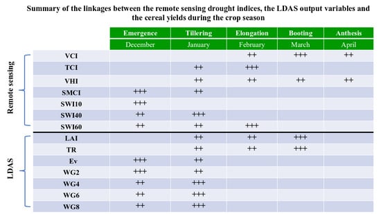
| Emergence | Tillering | Elongation | Booting | Anthesis | ||
|---|---|---|---|---|---|---|
| December | January | February | March | April | ||
| Remote sensing Drought indices | VCI | ++ | +++ | ++ | ||
| TCI | ++ | +++ | ||||
| VHI | ++ | ++ | ++ | ++ | ||
| SMCI | +++ | ++ | ||||
| SWI10 | +++ | |||||
| SWI40 | ++ | +++ | ||||
| SWI60 | ++ | ++ | +++ | |||
| LDAS outputs | LAI | ++ | ++ | +++ | ||
| Tr | ++ | ++ | +++ | |||
| Ev | +++ | ++ | ||||
| WG2 | +++ | ++ | ||||
| WG4 | ++ | +++ | ||||
| WG6 | ++ | +++ | ||||
| WG8 | ++ | +++ |
Publisher’s Note: MDPI stays neutral with regard to jurisdictional claims in published maps and institutional affiliations. |
© 2020 by the authors. Licensee MDPI, Basel, Switzerland. This article is an open access article distributed under the terms and conditions of the Creative Commons Attribution (CC BY) license (http://creativecommons.org/licenses/by/4.0/).
Share and Cite
Bouras, E.h.; Jarlan, L.; Er-Raki, S.; Albergel, C.; Richard, B.; Balaghi, R.; Khabba, S. Linkages between Rainfed Cereal Production and Agricultural Drought through Remote Sensing Indices and a Land Data Assimilation System: A Case Study in Morocco. Remote Sens. 2020, 12, 4018. https://doi.org/10.3390/rs12244018
Bouras Eh, Jarlan L, Er-Raki S, Albergel C, Richard B, Balaghi R, Khabba S. Linkages between Rainfed Cereal Production and Agricultural Drought through Remote Sensing Indices and a Land Data Assimilation System: A Case Study in Morocco. Remote Sensing. 2020; 12(24):4018. https://doi.org/10.3390/rs12244018
Chicago/Turabian StyleBouras, El houssaine, Lionel Jarlan, Salah Er-Raki, Clément Albergel, Bastien Richard, Riad Balaghi, and Saïd Khabba. 2020. "Linkages between Rainfed Cereal Production and Agricultural Drought through Remote Sensing Indices and a Land Data Assimilation System: A Case Study in Morocco" Remote Sensing 12, no. 24: 4018. https://doi.org/10.3390/rs12244018
APA StyleBouras, E. h., Jarlan, L., Er-Raki, S., Albergel, C., Richard, B., Balaghi, R., & Khabba, S. (2020). Linkages between Rainfed Cereal Production and Agricultural Drought through Remote Sensing Indices and a Land Data Assimilation System: A Case Study in Morocco. Remote Sensing, 12(24), 4018. https://doi.org/10.3390/rs12244018