A Novel Post-Doppler Parametric Adaptive Matched Filter for Airborne Multichannel Radar

Abstract

The post-Doppler adaptive matched filter (PD-AMF) with constant false alarm rate (CFAR) property was developed for adaptive detection of moving targets, which is a standardized version of the post-Doppler space–time adaptive processing (PD-STAP) in practical applications. However, its detection performance is severely constrained by the training data, especially in a dense signal environment. Improper training data and contamination of moving target signals remarkably degrade the performance of disturbance suppression and result in target cancellation by self-whitening. To address these issues, a novel post-Doppler parametric adaptive matched filter (PD-PAMF) detector is proposed in the range-Doppler domain. Specifically, the detector is introduced via the post-Doppler matched filter (PD-MF) and the lower-diagonal-upper (LDU) decomposition of the disturbance covariance matrix, and the disturbance signals of the spatial sequence are modelled as an auto-regressive (AR) process for filtering. The purpose of detecting ground moving targets as well as for estimating their geographical positions and line-of-sight velocities is achieved when the disturbance is suppressed. The PD-PAMF is able to reach higher performances by using only a smaller training data size. More importantly, it is tolerant to moving target signals contained in the training data. The PD-PAMF also has a lower computational complexity. Numerical results are presented to demonstrate the effectiveness of the proposed detector.

1. Introduction

Multichannel adaptive processing for airborne radar applications offers a powerful approach for signal detection in a background of correlated clutter plus additive white noise. For a variety of applications, space–time adaptive processing (STAP) for airborne radar is famous [1]. Conventional STAP detectors are typically developed for homogeneous environments, including Reed, Mallet, and Brennan detector [2]; Kelly’s generalized likelihood ratio test (GLRT) [3]; and the adaptive matched filter (AMF) detector [4], among others. These detectors’ disturbance suppression are carried out by inversion of the disturbance covariance matrix (DCM). However, in practical applications, since disturbance spectral properties are rarely known a priori, the DCM generally has to be estimated by using appropriate training data. In [2], a key result is the “Reed–Mullet–Brennan (RMB) rule”, which requires training data support so that 3-dB normalized signal-to-interference-and-noise ratio (SINR) performance is attained. Specifically, the RMB states that, for an array radar with M elements and N pulses, K = 2 MN − 3 ≈ 2 MN independent, identically distributed (I.I.D.), target-free training data vectors are needed to attain a performance corresponding to a 3-dB level below optimum. As the joint space–time dimension grows (increasing M or N), the training data size needs to increase dramatically, which can lead to excessive training and computational burden. Moreover, contamination of the training data with strong discrete scatterers and interfering moving target signals may remarkably degrade the performance. Therefore, the DCM estimation of conventional STAP is impractical in complex and changeable environments; many reduced dimensions or partial adaptive STAP algorithms have been proposed [5,6,7,8,9].

The post-Doppler space–time adaptive processing (PD-STAP) is a reduced rank algorithm of the classical joint domain STAP in the range-Doppler domain. The post-Doppler adaptive matched filter (PD-AMF) is a standardized version of PD-STAP and has the constant false alarm rate (CFAR) property in practical applications. First, doppler filtering is performed on the element signals; then, spatial adaptive beamforming is performed, that is, spatial whitening; and finally, target detection is achieved [5,9]. Compared with conventional STAP, PD-AMF has a wide application in the field of moving target detection due to the relatively small sample support requirement, especially in radar systems with longer coherent processing intervals (CPIs) and medium or large arrays [5]. Unfortunately, PD-AMF also has requirements for the training data size and content (i.e., RMB and I.I.D.). It is basically ineffective in a dense signal environment. More recently, a knowledge-aided (KA) algorithm showed that the generalized inner product (GIP) test can be applied in the space-Doppler domain in order to remove the nonhomogeneous training data from the DCM estimation. However, the use of KA algorithms further increases the complexity of STAP, especially when real-time processing is required [8,10].

In airborne radar applications, the disturbance usually exhibits certain spatial and temporal structures that can be exploited to ease the training and computational burden [11,12,13,14,15]. A general structured approach is to model the disturbance as an auto-regressive (AR) process, which has been found to be very useful in representing spatial and temporal correlations of radar signals [11]. The parametric STAP detector has been developed by the AR process, such as in parametric AMF (PAMF) [12], parametric Rao detector [13], and parametric generalized likelihood ratio test (PGLRT) [14,15]. They all operate in the space–time domain, and their computational burden increases significantly when the radar has a long CPI and a medium or large array. Recently, the PAMF detector has been shown to be equivalent to a parametric Rao detector [16].

The detection performance of PD-AMF is severely limited by training data, especially in a dense signal environment. Improper training data and contamination of moving target signals will remarkably degrade the performance of disturbance suppression and result in target cancellation by self-whitening. Moreover, the DCM inversion of most STAP detectors increase the computational burden. To address these issues, this paper proposes a novel post-Doppler parametric adaptive matching filter (PD-PAMF) detector for moving targets in the range-Doppler domain. The proposed PD-PAMF utilizes a parametric model to model the disturbance, which is different from the PD-AMF. It applies the AR process to whiten the spatial sequence of disturbance, which is also different from the PAMF modelling the time sequences as an AR process in the space–time. The AR coefficients are estimated from the spatial sequence and the K training data cells. These operations reduce the requirements of the training data size and content. Furthermore, as the disturbance is acquired by antennas with the same view angle and a time delay on the order of a millisecond, the spatial correlation is relatively high [17], and low-order AR model can accurately approximate the disturbance. More precisely, the AR order from 2 to 5 is sufficient [18,19]. Thus, the low-order AR model reduces the computational requirements. Specifically, it is demonstrated here that using only a small fraction of the training data required by the PD-AMF, the PD-PAMF offers dramatic improvement in detection performance over the PD-AMF. More importantly, it is excellent that the PD-PAMF is tolerant to the training data containing interfering moving target signals. It is also demonstrated that the computational efficiency of PD-PAMF is several times that of PD-AMF.

The remainder of this paper is organized as follows: Section 2 introduces the multichannel signal model and the PD-STAP framework. Section 3 modifies the conventional signal model to enhance the generality of the proposed detector and derives the post-Doppler parametric matched filter (PD-PMF) detector. Section 4 models the AR process and derives the PD-PAMF detector in practical applications. Section 5 presents numerical evaluation to demonstrate the effectiveness of the PD-PAMF detector compared with the existing PD-PAMF detector. Section 6 presents a brief discussion about the limitations of the proposed PD-PAMF in real applications. Finally, Section 7 contains our conclusion.

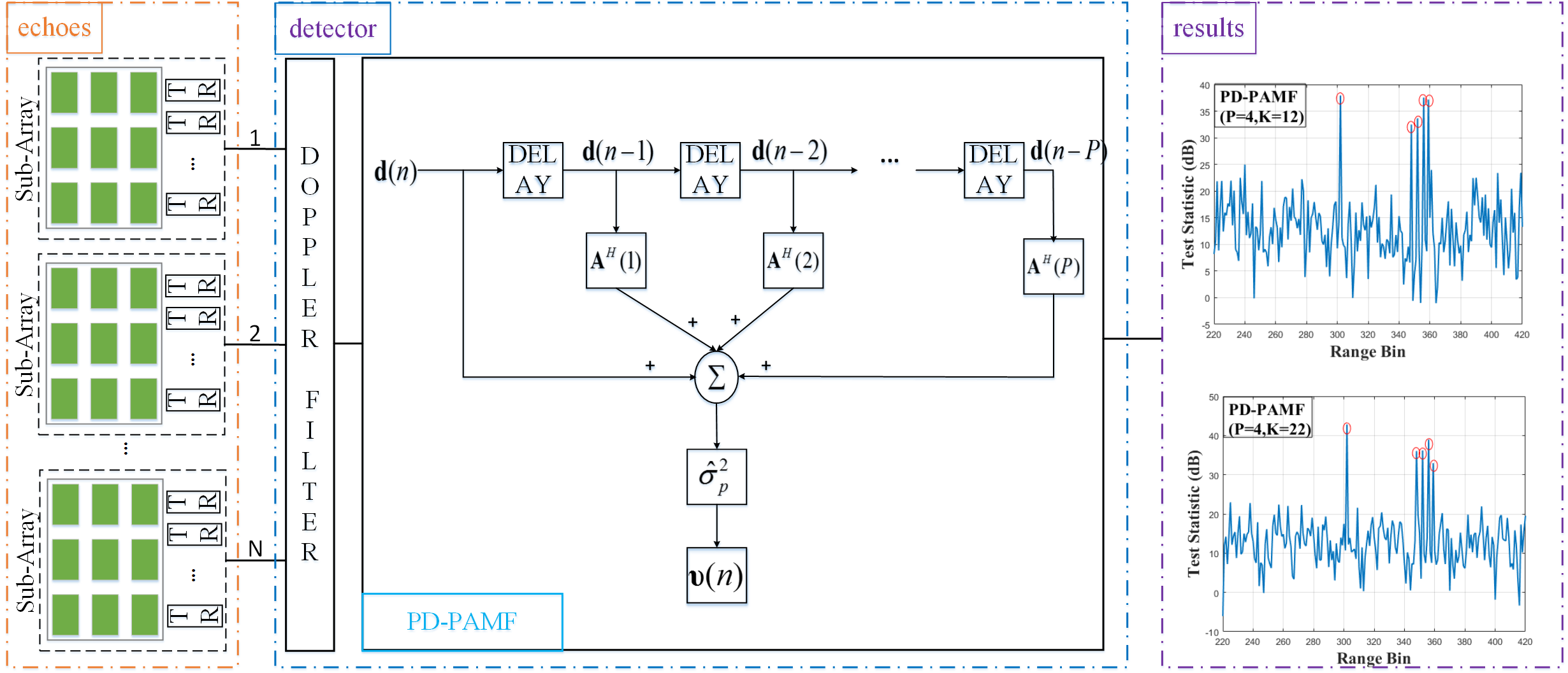
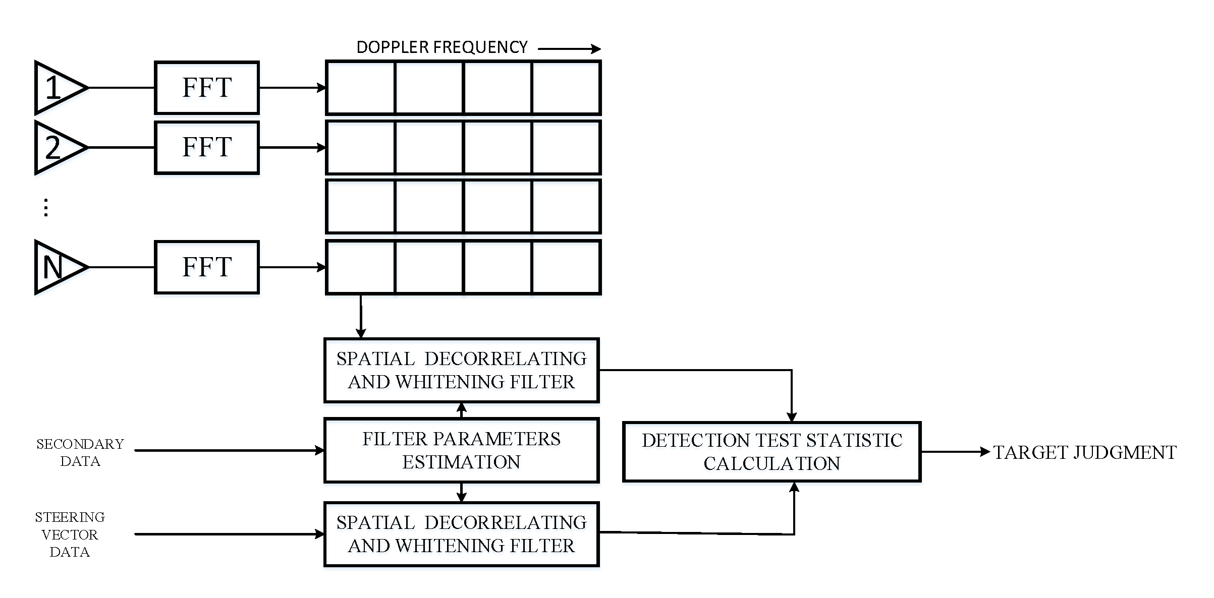
2. Multichannel Signal Model and PD-STAP Overview

The PD-STAP is a reduced rank algorithm of the classical joint domain STAP, which is mainly carried out in the range-Doppler domain. A moving target should remain in one doppler cell during the integration time to optimize the computational cost (STAP processing) [5,7,8]. Otherwise, the long CPI needs to be divided into shorter CPIs for processing. Assume that the airborne radar system has N channels in azimuth. The first channel serves as a reference channel. The physical baseline length of the nth channel is $b_n$, with n = 1,…, N and $b_1=0$. Assume $b_n\ll Ha$, which is the platform distance from the ground.

The multichannel signal model for the PD-STAP is as follows [8,9]:

$$\mathbf{s}\left(u\left(t\right)\right)=\alpha e^{-2j\beta R\left(t\right)}\left[\begin{array}{c}{D}_1\left(u\left(t\right)\right)e^{-j\beta u\left(t\right){\mathrm{b}}_1}\\ D_2\left(u\left(t\right)\right)e^{-j\beta u\left(t\right)b_2}\\ ⋮\\ D_N\left(u\left(t\right)\right)e^{-j\beta u\left(t\right)b_N}\end{array}\right]=\alpha e^{-2j\beta R\left(t\right)}\mathbf{e}\left(u\right)$$

(1)

where $\alpha$ denotes the complex amplitude of the reflectivity of the scatterer; $\beta ={\displaystyle \frac{2\pi }{\lambda }}$ is the wavenumber; $\lambda$ is the radar wavelength; $D_n$, with $n=1,\dots ,N$, is the two-way characteristics of the nth antenna; $\mathbf{e}\left(u\right)$ is the space steer vector; $u\left(t\right)=cos\left(\theta \right)$ is the directional cosine; and $\theta$ is the direction of arrival (DOA) since the squint angle is assumed zero, as shown in Figure 1. Vectors (matrices) are denoted by boldface lower (upper) case letters.

Since the directional cosine of the target is related to its doppler frequency and line-of-sight velocity, it can be expressed as follows:

$${\mathrm{u}}_t(f_a,v_r)=cos\left(\theta \right)=\frac{\lambda f_a}{2V}+\frac{v_r}{V}$$

(2)

where $f_a$ is the doppler frequency bin, $v_r$ is the line-of-sight velocity, and V is the platform velocity.

In the range-Doppler domain, the binary hypothesis can be written as follows [20]:

$$\left\{\begin{array}{c}{H}_0:\mathbf{x}\left(f_a\right)=\mathbf{d}\left(f_a\right),Movingtargetisabsent\hfill \\ H_1:\mathbf{x}\left(f_a\right)=\alpha \mathbf{e}({\mathrm{u}}_t,f_a)+\mathbf{d}\left(f_a\right),Movingtargetispresent\hfill \end{array}\right.$$

(3)

where all vectors are $N\times 1$ vectors:

$$\begin{array}{c}\mathbf{x}\left(f_a\right)={[x(1,f_a),x(2,f_a),\cdots ,x(N,f_a)]}^T\hfill \\ \mathbf{d}\left(f_a\right)={[d(1,f_a),d(2,f_a),\cdots ,d(N,f_a)]}^T\hfill \\ \mathbf{e}\left(f_a\right)={[e(1,f_a),e(2,f_a),\cdots ,e(N,f_a)]}^T\hfill \end{array}$$

(4)

${[·]}^T$ denotes the matrix transpose; $x(\mathrm{n},f_a),e(\mathrm{n},f_a)$, and $d(\mathrm{n},f_a)$, with $n=1,\dots ,N$, are the test signal, the detected signal, and the disturbance signal, respectively; $\mathbf{e}$ is the signal vector with amplitude $\alpha$; and $\mathbf{d}$ is the disturbance vector with positive definite covariance matrix ${\mathbf{R}}_d\in {\mathbb{C}}^{N\times N}$ and consists of ground clutter $\mathbf{c}$, interference $\mathbf{i}$, and thermal white noise $\mathbf{w}$ with covariance matrices ${\mathbf{R}}_c$, ${\mathbf{R}}_i$, and ${\mathbf{R}}_w$, respectively. It is assumed that the disturbance components are additive and pairwise independent and that each is a stationary, zero-mean Gaussian-distributed process. Thus, ${\mathbf{R}}_d={\mathbf{R}}_c+{\mathbf{R}}_i+{\mathbf{R}}_w$, and $\mathbf{x}\sim CN(\alpha \mathbf{e},{\mathbf{R}}_{\mathbf{d}})$, with $\alpha =0$ under $H_0$.

For known ${\mathbf{R}}_d$ and $\mathbf{e}$ and unknown $\alpha$, the moving target detection is carried out by applying post-Doppler matched filter test (PD-MF) [4]:

$${\mathsf{\Lambda }}_{PD-MF}=\frac{|{\mathbf{e}}^H({\mathrm{u}}_t,f_a){\mathbf{R}}_d^{-1}\left(f_a\right)\mathbf{x}\left(f_a\right){|}^2}{{\mathbf{e}}^H({\mathrm{u}}_t,f_a){\mathbf{R}}_d^{-1}\left(f_a\right)\mathbf{e}({\mathrm{u}}_t,f_a)}$$

(5)

In general, ${\mathbf{R}}_{\mathbf{d}}$ and $\mathbf{e}$ are also unknown, $\mathbf{e}$ is usually searched within a velocity range, and the covariance matrix is unknown and must be estimated by using adaptive techniques:

$${\widehat{\mathbf{R}}}_d\left(f_a\right)=\frac{1}{K}\sum _{k=1}^K{\mathbf{x}}_k\left(f_a\right){\mathbf{x}}_k^H\left(f_a\right)$$

(6)

${[·]}^H$ denotes matrix conjugate transpose, ${\mathbf{x}}_k\left(f_a\right)$ is the kth secondary data at the doppler bin $f_a$, and K is the training data size. For the PD-AMF test, substitute the estimated ${\widehat{\mathbf{R}}}_d\left(f_a\right)$ in Equation (6) to replace the unknown covariance ${\mathbf{R}}_d\left(f_a\right)$ in Equation (5). It is important to notice that the training data should meet the I.I.D. rule; otherwise, the detection performance will be greatly degraded. Thus, the application of PD-AMF is limited due to the requirement of training data, and it may be invalid in a dense signal environment. Therefore, this paper proposes the PD-PAMF in order to address the detection issues in the scene with limited training data.

3. Post-Doppler Parametric Matched Filter

In this section, the aforementioned multichannel signal model is modified in order to enhance the versatility of the proposed detector, such as the application of the nonuniform array radar. Then, based on the PD-MF and the lower-diagonal-upper (LDU) decomposition of the DCM, a post-Doppler parametric matched filter (PD-PMF) is obtained.

3.1. Modified Multichannel Signal Model

From Section 2, we realize that the phase difference among the channels can be partially compensated before the PD-MF process and only the phase difference caused by the target is retained [21].

$$\begin{array}{cc}\hfill \Delta {\varphi }_{1n}& =e(1,f_a)e^{*}(n,f_a)=\Delta D_{1n}\left(u\left(t\right)\right)e^{j\beta u\left(t\right)\left({\mathrm{b}}_n-{\mathrm{b}}_1\right)}\hfill \\ \hfill & =\Delta D_{1n}\left(u\left(t\right)\right)e^{j2\pi f_a\frac{{\mathrm{b}}_n}{2V}+j2\pi \frac{2v_r}{\lambda }\frac{{\mathrm{b}}_n}{2V}}\hfill \\ \hfill & =\Delta D_{1n}\left(u\left(t\right)\right)e^{j2\pi f_a{t}_n}{e}^{j2\pi \frac{2v_r}{\lambda }{t}_n}\hfill \end{array}$$

(7)

where $\Delta {\varphi }_{1n}$, $\Delta D_{1n}\left(u\left(t\right)\right)$, ${\mathrm{b}}_n$, and $t_n$,$(n=1,\dots ,N)$ denote the phase difference of the signal to be detected, antenna transceiver characteristics, effective baseline, and baseline delay time between the first and nth channel, respectively. Equation (7) shows that the phase differences between elements of $\mathbf{e}$ are composed of three items: the first item is produced by the antenna’s transceiver characteristics, the second item is produced by the baseline delay between channels, and the third item is produced by the moving target velocity. ${[·]}^{*}$ denotes the conjugate. After baseline delay correction, the multichannel signal model can be written as follows:

$$\mathbf{s}\left(v_r\right)=\alpha c{e}^{-2j\beta R\left(t\right)}\left[\begin{array}{c}{e}^{-j2\pi \frac{2v_r}{\lambda }{t}_1}\\ e^{-j2\pi \frac{2v_r}{\lambda }{t}_2}\\ ⋮\\ e^{-j2\pi \frac{2v_r}{\lambda }{t}_N}\end{array}\right]=\alpha c{e}^{-2j\beta R\left(t\right)}\mathbf{e}\left(v_r\right)$$

(8)

Since $t_n$ is fixed and c is the constant phase after multichannel phase compensation, the elements of the target signal steer vector are only related to $v_r$. For a stationary target ($v_r=0$ m/s), $\mathbf{e}\left(v_r\right)$ is equal to ${\mathbf{1}}_N$, which is the all-ones N-dimensional column vector. However, in practical applications, data preprocessing is necessary in order to improve the detection performance. The preprocessing contains platform motion compensation [22,23], antenna pattern calibration [24], phase compensation [25], and baseline delay correction [21,26]. We utilize traditional methods for data preprocessing, which is not the main research content of this paper.

3.2. Post-Doppler Parametric Matched Filter Derivation

To better understand PD-PAMF, we derive its expression form from PD-MF. For the signal model in Equation (8), the form of PD-MF is as follows:

$${\mathsf{\Lambda }}_{PD-MF}=\frac{|{\mathbf{e}}^H\left(v_r\right){\mathbf{R}}_d^{-1}\left(f_a\right)\mathbf{x}\left(f_a\right){|}^2}{{\mathbf{e}}^H\left(v_r\right){\mathbf{R}}_d^{-1}\left(f_a\right)\mathbf{e}\left(v_r\right)}$$

(9)

All variables in Equation (9) are distinct to those of the detection statistics in Equation (5), but the same symbols are utilized for notational simplicity.

The PD-MF and PD-AMF detection statistics admit various interpretations. One explanation is derived from the matrix square-root decomposition (Cholesky) of the DCM. Since ${\mathbf{R}}_d$ is Hermitian symmetric, the factorization can be written as follows:

$${\mathbf{R}}_d=\mathbf{A}{\mathbf{A}}^H$$

(10)

where A is a lower triangular matrix. The inversion of ${\mathbf{R}}_d$ is as follows:

$${\mathbf{R}}_d^{-1}={\left(\mathbf{A}{\mathbf{A}}^H\right)}^{-1}={\left({\mathbf{A}}^H\right)}^{-1}{\mathbf{A}}^{-1}$$

(11)

Then, ${\mathsf{\Lambda }}_{PD-MF}$ can be rewritten as follows:

$${\mathsf{\Lambda }}_{PD-MF}=\frac{|{\mathbf{e}}^H\left(v_r\right){\left(\mathbf{A}{\mathbf{A}}^H\right)}^{-1}\mathbf{x}\left(f_a\right){|}^2}{{\mathbf{e}}^H\left(v_r\right){\left(\mathbf{A}{\mathbf{A}}^H\right)}^{-1}\mathbf{e}\left(v_r\right)}=\frac{|{\left({\mathbf{A}}^{-1}\mathbf{e}\left(v_r\right)\right)}^H{\mathbf{A}}^{-1}\mathbf{x}\left(f_a\right){|}^2}{{\left({\mathbf{A}}^{-1}\mathbf{e}\left(v_r\right)\right)}^H\left({\mathbf{A}}^{-1}\mathbf{e}\left(v_r\right)\right)}=\frac{|{\mathbf{y}}^H\nu {|}^2}{{\mathbf{y}}^H\mathbf{y}}$$

(12)

where $\nu$ represents the whitening of the interference components in $\mathbf{x}\left(f_a\right)$ and $\mathbf{y}$ represents the pre-distortion of the steer vector by a linear transformation ${\mathbf{A}}^{-1}$. This transformation ensures that the steer vector $\mathbf{e}\left(v_r\right)$ actually matches the underlying signal components in the transformed data vector $\nu$.

Another interpretation is the LDU decomposition of the DCM, which emphasizes the relationship with linear prediction, and this factorization is meaningful. It is also the main motivation for proposing the PD-PMF. Moreover, this method is also applicable to PD-PAMF [12,27].

Since ${\mathbf{R}}_d$ is Hermitian symmetric, its LDU decomposition can be written as follows:

$${\mathbf{R}}_d=\mathbf{AD}{\mathbf{A}}^H$$

(13)

$${\mathbf{A}}^{-1}=\left[\begin{array}{cccc}1& 0& \cdots & 0\\ a_2\left(1\right)& 1& \cdots & 0\\ ⋮& ⋮& \ddots & ⋮\\ a_N(N-1)& a_N(N-2)& \cdots & 1\end{array}\right]$$

(14)

$$\mathbf{D}=\left[\begin{array}{cccc}{\sigma }_1^2& 0& \cdots & 0\\ 0& {\sigma }_2^2& \cdots & 0\\ ⋮& ⋮& \ddots & ⋮\\ 0& 0& \cdots & {\sigma }_N^2\end{array}\right]$$

(15)

where $\mathbf{A}$ is a lower triangular matrix with unity elements along the main diagonal and $\mathbf{D}$ is a diagonal matrix with positive elements along the main diagonal. The forms of ${\mathbf{A}}^{-1}$ and $\mathbf{D}$ are referenced from Equations (14) and (15). The rows of ${\mathbf{A}}^{-1}$ are the coefficients of linear prediction, and the elements of $\mathbf{D}$ are the prediction error variances. Thus, ${\mathsf{\Lambda }}_{PD-MF}$ can be expressed as follows:

$$\begin{array}{cc}\hfill {\mathsf{\Lambda }}_{PD-MF}& =\frac{|{\mathbf{e}}^H\left(v_r\right){\left(\mathbf{AD}{\mathbf{A}}^H\right)}^{-1}\mathbf{x}\left(f_a\right){|}^2}{{\mathbf{e}}^H\left(v_r\right){\left(\mathbf{AD}{\mathbf{A}}^H\right)}^{-1}\mathbf{e}\left(v_r\right)}\hfill \\ \hfill & =\frac{|{({\mathbf{D}}^{{}^{-1/\phantom{-12}2}}{\mathbf{A}}^{-1}\mathbf{e}(v_r))}^H({\mathbf{D}}^{{}^{-1/\phantom{-12}2}}{\mathbf{A}}^{-1}\mathbf{x}(f_a)){|}^2}{{({\mathbf{D}}^{{}^{-1/\phantom{-12}2}}{\mathbf{A}}^{-1}\mathbf{e}(v_r))}^H({\mathbf{D}}^{{}^{-1/\phantom{-12}2}}{\mathbf{A}}^{-1}\mathbf{e}(v_r))}\hfill \\ \hfill & =\frac{|{({\mathbf{D}}^{{}^{-1/\phantom{-12}2}}\mathbf{u})}^H({\mathbf{D}}^{{}^{-1/\phantom{-12}2}}\epsilon ){|}^2}{{({\mathbf{D}}^{{}^{-1/\phantom{-12}2}}\mathbf{u})}^H({\mathbf{D}}^{{}^{-1/\phantom{-12}2}}\mathbf{u})}\hfill \\ \hfill & =\frac{|{\mathbf{y}}^H\nu {|}^2}{{\mathbf{y}}^H\mathbf{y}}\hfill \end{array}$$

(16)

where $\mathbf{y}$ represents the pre-distortion of the steer vector by a linear transformation ${\mathbf{D}}^{{}^{-1/\phantom{-12}2}}{\mathbf{A}}^{-1}$ in order to ensure that the steer vector matches the underlying signal components in the $\mathbf{\nu }$. The elements of vector $\mathbf{\epsilon }$ and vector $\mathbf{\nu }$ are $\epsilon \left(n\right)$ and $\nu \left(n\right)$, respectively. They are given by

$$\epsilon \left(n\right)=\sum _{p=0}^{n-1}{a}_n\left(p\right)x(n-p,f_a),n=1,\dots ,N$$

(17)

$$\nu \left(n\right)=\frac{1}{{\sigma }_n}\epsilon \left(n\right)=\frac{1}{{\sigma }_n}\sum _{p=0}^{n-1}{a}_n\left(p\right)x(n-p,f_a),n=1,...,N$$

(18)

where $a_n\left(0\right)=1$ for all n. Equation (17) shows that $\epsilon \left(n\right)$ is the output of nth-order moving-average (MA) filter. Since these filter coefficients are linear prediction coefficients, there is no correlation between the prediction error sequences $\left\{\epsilon \right(n\left)\right|n=1,...,N\}$ and their covariance matrix is diagonal matrix $\mathbf{D}$, i.e., $\mathbf{D}=E\left\{\mathbf{\epsilon }{\mathbf{\epsilon }}^H\right\}$. Thus, ${\mathbf{A}}^{-1}$ is a decorrelating step in spatial dimension and ${\mathbf{D}}^{{}^{-1/\phantom{-12}2}}$ is a whitening step (i.e., $\upsilon \left(n\right)=1,n=1,\dots ,N$). Similar expressions are obtained for the steer vectors $\mathbf{u}$ and $\mathbf{y}$.

In the range-Doppler domain, the spatial sequences are highly correlated. Thus, both $\mathbf{\epsilon }$ and $\nu$ retain only the vector sequence for the filter of order P, where $1\le P\le N$ [12]. Further, setting the MA filter as a moving window, the spatial filter has the following form:

$$\upsilon \left(n\right)=\frac{1}{\sqrt{{\sigma }_P^2}}\epsilon \left(n\right)=\frac{1}{\sqrt{{\sigma }_P^2}}\sum _{p=0}^{P}a\left(p\right)x(n-p+P,f_a),n=1,...,N-P$$

(19)

Equation (19) is rewritten as the form of a matrix:

$$\nu =\frac{1}{\sqrt{{\sigma }_P^2}}\epsilon =\frac{1}{\sqrt{{\sigma }_P^2}}\left(\mathbf{x}\left(f_a\right)\mathbf{A}\right)$$

(20)

where

$$\mathbf{x}\left(f_a\right)=\left[\begin{array}{cccc}x(1,f_a)& x(2,f_a)& \cdots & x(N-P,f_a)\\ x(2,f_a)& x(3,f_a)& \cdots & x(N-P+1,f_a)\\ ⋮& ⋮& \cdots & ⋮\\ x(P+1,f_a)& x(P+2,f_a)& \cdots & x(N,f_a)\end{array}\right]$$

(21)

$$\mathbf{A}={\left[\begin{array}{cccc}a\left(P\right)& a(P-1)& \cdots & a\left(0\right)\end{array}\right]}^T$$

(22)

where $a\left(p\right),p=0,\dots ,P$ is the coefficient and $a\left(0\right)=1$; $\nu \in {\mathbb{C}}^{1\times (N-P)}$ is the whiting vector of the test signal; ${\sigma }_P^2$ is the Pth-order predictor error (i.e., the element of the diagonal $\mathbf{D}$ in Equation (15)); A is the Pth-order prediction coefficient vector; and $\mathbf{x}\left(f_a\right)$ is the spatial sequence vector. Considering the number of symbols, the filter output defined above has the same symbol as the corresponding variable in PD-MF. The sequence $\left\{\epsilon \right(n\left)\right|n=1,...,N-P\}$ is the output of an MA filter with input sequence $\left\{x(f_a,n)\right|n=1,...,N-P\}$, which is referred to as the spatial residual sequence. The output of the MA filter is not correlated (i.e., ${\mathbf{R}}_{\epsilon }=E\left\{\mathbf{\epsilon }{\mathbf{\epsilon }}^H\right\}={\sigma }^2{\mathbf{I}}_{N-P}\in {\mathbb{C}}^{(N-P)\times (N-P)}$). Therefore, the sequence $\left\{\nu \right(n\left)\right|n=1,\dots ,N-P\}$ is also uncorrelated and its variance is 1 (i.e., ${\mathbf{R}}_{\nu }=E\left\{\mathbf{\nu }{\mathbf{\nu }}^H\right\}={\mathbf{I}}_{N-P}\in {\mathbb{C}}^{(N-P)\times (N-P)}$, where $\mathbf{I}$ is the identity matrix ).

The steering sequence is filtered analogously. The vector $\mathbf{e}\left({\mathbf{v}}_{\mathbf{r}}\right)$ has been changed to the following:

$$y\left(n\right)=\frac{1}{\sqrt{{\sigma }_P^2}}u\left(n\right)=\frac{1}{\sqrt{{\sigma }_P^2}}\sum _{p=0}^{P}a\left(p\right)e(n-p+P,v_r),n=1,\dots ,N-P$$

(23)

Rewriting Equation (23), we have the following:

$$\mathbf{y}=\frac{1}{\sqrt{{\sigma }_P^2}}\mathbf{u}=\frac{1}{\sqrt{{\sigma }_P^2}}\left(\mathbf{e}\left(v_r\right)\mathbf{A}\right)$$

(24)

where

$$\mathbf{e}(v_r)=\left[\begin{array}{cccc}e(1,v_r)& e(2,{v_r}_a)& \cdots & e(N-P,v_r)\\ e(2,v_r)& e(3,v_r)& \cdots & e(N-P+1,v_r)\\ ⋮& ⋮& \cdots & ⋮\\ e(P+1,v_r)& e(P+2,v_r)& \cdots & e(N,v_r)\end{array}\right]$$

(25)

where ${\sigma }_P^2$ and $\mathbf{A}$ are the same as in Equations (20) and (22). $\mathbf{y}\in {\mathbb{C}}^{\mathbf{1}\times (\mathbf{N}-\mathbf{P})}$ denotes the steer vector after filter. Based on the above discussion, the PD-PMF detection statistic ${\mathsf{\Lambda }}_{PD-PMF}$ is defined as follows:

$${\mathsf{\Lambda }}_{PD-PMF}=\frac{|{\mathbf{y}}^H\nu {|}^2}{{\mathbf{y}}^H\mathbf{y}}\underset{H_1}{\overset{H_0}{{}_{>}^{<}}}\gamma$$

(26)

where $\mathbf{y}$ and $\nu$ are from the Equations (20) and (24), respectively. $\gamma$ is the detection threshold. If $\mathbf{A}$ and $\mathbf{D}$ are known, then we would use the detector described by Equation (26). In general, they are not known and must be accounted for by using adaptive techniques. This is the PD-PAMF detector that will be introduced in the next section.

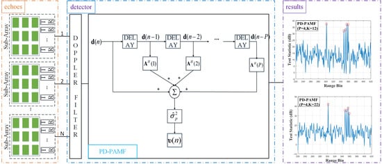
4. Post-Doppler Parametric Adaptive Matched Filter

4.1. Post-Doppler Parametric Adaptive Matched Filter Derivation

As indicated by the LDU decomposition of DCM, the AR model is a natural model type of PD-PAMF. When the filter parameters are unknown, they must be estimated adaptively. Literatures on using AR processes to model interference in radar systems are very rich [11,12,18,19,28]. It has been found from a large amount of experiments that the low-order AR process can be used to accurately and effectively approximate the radar interference [19]. Herein, we use the AR process to model the disturbance $\mathbf{d}\left(f_a\right)$, which is a complex Gaussian-distributed with zero-mean:

$$\mathrm{d}(n,f_a)=-\sum _{p=1}^{P}a\left(p\right)\mathrm{d}(n-p,f_a)+\epsilon \left(p\right),n=1,\dots ,N$$

(27)

where $\mathrm{d}(n,f_a)$ denotes the nth channel, $\epsilon \left(p\right)\sim CN(0,{\sigma }_P^2)$ is the zero-mean driving noise with variance ${\sigma }_P^2$, $a\left(p\right)$ is the pth AR coefficient, and P is the AR model order. The AR process of order P denotes AR(P). In this paper, we assume that P is known. Otherwise, it can be estimated by using a variety of model order selection techniques (e.g., Akaike information criterion (AIC) [29] and Rissanen’s minimum description length (MDL) [30]). For stability, all system poles must lie inside the unit circle in the complex plane.

The AR(P) system is causally and causally reversible, so the following form of inverse system (whitening filter) is allowed:

$$\epsilon \left(n\right)=\sum _{p=0}^{P}a\left(p\right)d(n-p,f_a),n=1,\dots ,N-P$$

(28)

where $a\left(0\right)=1$. Equation (28) shows that $\left\{\epsilon \right(n\left)\right|n=1,...,N\}$ is the MA process of order P and $\left\{a\right(p\left)\right|p=0,...,P\}$ is the prediction coefficients of MA process. MA is also a causal system, so it is causally reversible. For a given system order, the number of AR(P) (or MA(P)) complex-valued parameters is P. We can use the Strand–Nuttall AR model identification algorithm or the least squares AR model identification algorithm to estimate the prediction parameters. In comparison, the least square AR model identification algorithm has the better performance [12]. This paper utilizes this method to estimate the prediction coefficients by training data, which is denoted as $\widehat{\mathbf{A}}$ (for details, please refer to [27]), and the corresponding elements are marked as $\widehat{a}\left(p\right),p=1,...,P$.

The predictor error ${\sigma }_P^2$ of the spatial residual sequence can be directly determined by using the parameter estimation algorithm [31]. However, once the AR model does not meet the decorrelation condition (i.e., the sequence $\left\{\epsilon \right(n\left)\right|n=1,...,N-P\}$ is correlative), the output sequence $\left\{\nu \right(n\left)\right|n=1,...,N-P\}$ of the filter is colored, which will result in insufficient whitening [12]. Fortunately, improved detection and CFAR performance can be achieved when both space and range cell averaging of the outer products of $\mathbf{\epsilon }\left(n\right)$ are used to estimate this error [32,33]. Thus, the predictor error is given by the following:

$${\widehat{\sigma }}_P^2=\frac{1}{K(N-P)}\sum _{n=1}^{N-P}\sum _{k=1}^K{\epsilon }_{k|H_0}\left(n\right){\epsilon }_{k|H_0}^H\left(n\right)$$

(29)

where the argument k denotes the kth secondary range bin and K is the training data size. Using $\widehat{\mathbf{A}}$ and ${\widehat{\sigma }}_P^2$ to substitute into Equations (20) and (24), respectively, we obtain the following:

$$\upsilon =\frac{1}{\sqrt{{\widehat{\sigma }}_P^2}}(\mathbf{x}(f_a)\widehat{\mathbf{A}})$$

(30)

$$\mathbf{y}=\frac{1}{\sqrt{{\widehat{\sigma }}_P^2}}(\mathbf{e}(v_r)\widehat{\mathbf{A}})$$

(31)

From the above analysis, the test statistics of PD-PAMF can be obtained in the following form:

$${\mathsf{\Lambda }}_{PD-PAMF}=\frac{|{\mathbf{y}}^H\nu {|}^2}{{\mathbf{y}}^H\mathbf{y}}\underset{H_1}{\overset{H_0}{{}_{>}^{<}}}\gamma$$

(32)

where $\gamma$ is the detection threshold. Equations (26) and (32) have the same form, but the prediction coefficient matrix and prediction error variance of Equation (26) are known,while Equation (32) is adaptively estimated from the training data. Only for the simplicity of notation, the same notation is used.

The above discussions are based on the assumption of a given target velocity (i.e., the steering vector $\mathbf{e}\left(v_r\right)$ is determined). In practice, this may correspond to the case when multiple detections are performed on a set of possible values of the target $v_r$, equivalently, the doppler frequencies. Alternatively, we can treat the target velocity $v_r$ as an unknown parameter which needs to be estimated before detection. In this case, the test variable of the PD-PAMF detector can be expressed as follows:

$${\mathsf{\Lambda }}_{PD-PAMF}={}_{v_r}^{max}\frac{|{\mathbf{y}}^H\nu {|}^2}{{\mathbf{y}}^H\mathbf{y}}\underset{H_1}{\overset{H_0}{{}_{>}^{<}}}\gamma$$

(33)

Once the test cell has a target (satisfying $H_1$), the estimated velocity ${\widehat{v}}_r$ of the moving target can be obtained by Equation (33) and then its DOA can be calculated by Equation (2) for positioning. The PD-PAMF can be implemented as a tapped delay line, and the tap weight is given by 1 and $-\widehat{a}\left(p\right),p=1,...,P$ and has a simple structure that can be easily changed with the change of $\widehat{a}\left(p\right)$. This was one of the motivating factors in modeling disturbance as an AR process. Therefore, PD-AMF has a wide range of application potentials in the field of airborne radar moving target detection. The processing structure of the PD-PAMF detector is illustrated in Figure 2.

4.2. Computational Complexity

In real-time applications, the computational burden is particularly important. We analyze the computational complexity of the PD-PAMF in detail. Compared with PD-AMF, PD-PAMF is computationally simpler since it has lower requirements on the training data size and does not involve DCM inversion. Specifically, supposing that the AR order (generally, 2∼5 order) and the target velocity are known (the computational cost of these methods for estimating target velocity is similar) and considering that using the least square AR model identification algorithm and disregarding the common computational cost for the two detectors, the proposed detector has a complexity of $O(K{P}^3+K)$ while the PD-AMF has a complexity of $O(K{N}^2+N^3)$ [34], the complexity $O\left(K{P}^3\right)$ of the PD-PAMF is due to AR prediction coefficients of K range bins and the complexity $O\left(K\right)$ is the average of K coefficients. The complexity $O\left(K{N}^2\right)$ of the PD-AMF is due to the DCM estimation in Equation (6), and the complexity $O\left(N^3\right)$ is due to the inversion of the $N\times N$ estimated DCM.

5. Numerical Evaluation

To assess the detection and estimation performance of the proposed PD-PAMF, we present the results of the theoretical performance and the experiments of simulated airborne multichannel radar data in a dense signal environment. In the different experiments, the performance of PD-PAMF is compared with PD-AMF and optimal PD-MF. The SINR is defined as $SINR=|\alpha {|}^2{\mathbf{e}}^H{\mathbf{R}}_d^{-1}\mathbf{e}$. ${\theta }_t$ and $v_{rt}$ are referred to as the DOA and the line-of-sight velocity of moving targets, respectively. The corresponding normalized doppler is $f_{td}=2{v_r}_t/\phantom{2{v_r}_t(\lambda PRF}(\lambda PRF)$, where PRF is the pulse repetition frequency. In this paper, we use a uniform linear array radar to do the experiments. The antenna separation is b, and the corresponding physical baseline is $b_i$ ($b_n=(n-1)b,n=1,\dots N$).

5.1. Theoretical Performance

The theoretical performance of the PD-PAMF is studied via computer simulation. In other words, using the Monte Carlo simulation method to evaluate the estimation of the detection probability ($P_D$) and velocity under different conditions. Part of the simulation parameters are shown in

Table 1. Simulation Parameters.

Parameters	Variables	Values
Wavelength	$\lambda$	0.03 m
Platform velocity	V	100 m/s
Number of channels	N	11
Antenna separation	b	0.1 m
Target direction of arrival	${\theta }_t$	90${}^{\circ }$
Target radial velocity	$v_{rt}$	1 m/s
Pulse repetition frequency	PRF	1000 Hz
Clutter to noise ratio	CNR	10 dB

. The target with ${\theta }_t={90}^o$ and $v_{rt}=1m/s$ is tested, and the main beam angle of the radar is 90${}^{\circ }$ (i.e., side-looking radar). The clutter to noise ratio (CNR) is 10 dB.

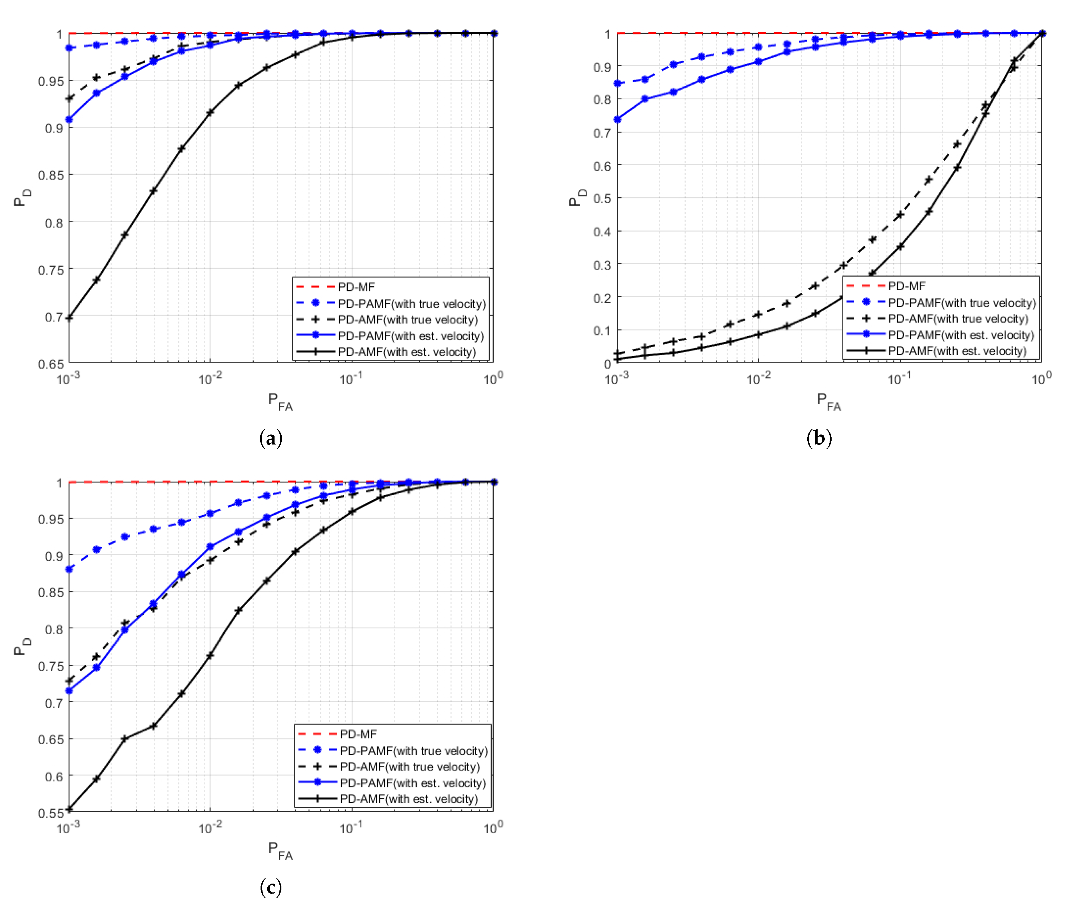
5.1.1. Receiver Operating Characteristic (ROC) Curves

Figure 3a–c shows the ROC curves of the relationship between the $P_D$ and the false alarm probability ($P_{FA}$ ). The simulation parameters SINR is 13 dB, and PD-MF (red dashed line) is used as the best performance reference curve. The ROC curve is obtained through a Monte Carlo experiment of ${10}^4$ repetitions. The blue and black solid lines indicate the unknown target velocity, which is obtained by searching over the range of the target velocity, and the blue and the black dashed line are obtained by the known target velocity. As we can see, compared with their detection performance of known target parameters, both PD-PAMF and PD-AMF have a certain performance loss, which is caused by their parameter estimation step. Among them, Figure 3a is the ROC obtained under K = 2 N = 22 training data, the size of which conforms to the RMB rule. It can be seen that, when the target velocity is known, the performances of the PD-PAMF and the PD-AMF are basically similar and are close to the performance of the PD-MF. However, when the target velocity is unknown, the performance of PAMF degrades a little, while PD-AMF degrades obviously. Thus, the PD-PAMF outperforms the PD-AMF. Figure 3b is obtained in the case of K = 8, that is, for the PD-AMF, the training data is insufficient, so we see a sharp decline in PD-AMF detection performance regardless of known or unknown target velocity. Compared with the training data K = 22, the performance loss of PD-PAMF is very small, which is closer to PD-MF. Figure 3c simulates the dense signal environment, and the training data contains the moving target signal (the same parameters as the moving target signal to be detected). The training data size of the PD-PAMF detector is K = 8, and the PD-AMF is K = 22. The results show that the detection performance of PD-AMF generally has no loss, while the performance loss of PD-AMF is more serious than that in Figure 3a, which may be caused by self-whitening. In other words, the PD-PAMF tolerates the moving target signal in the training data.

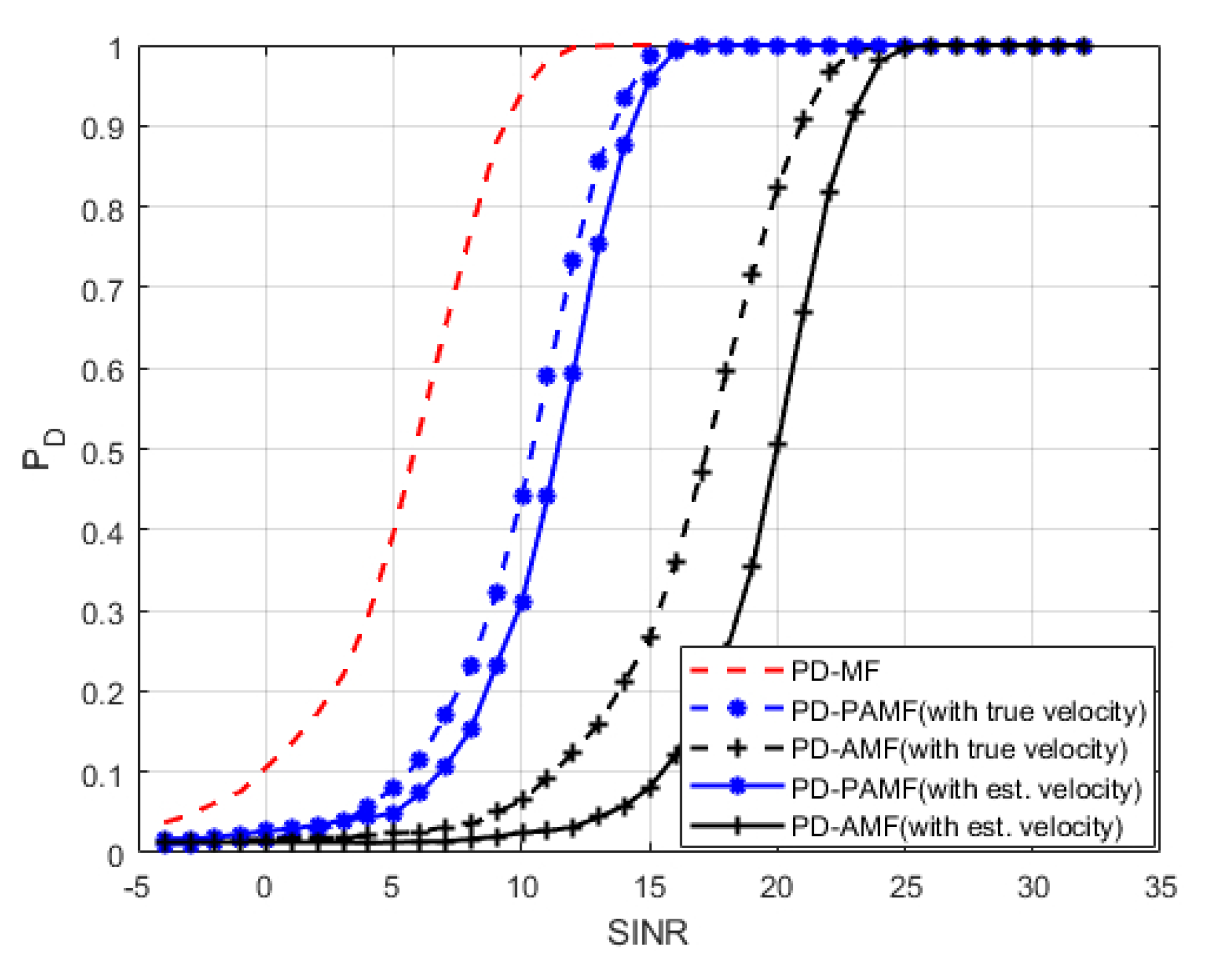
5.1.2. Probability of Detection versus SINR

Then, in Figure 4, we study the effect of SINR on $P_D$. In order to limit the computational burden, $P_{FA}$ is chosen under ${10}^{-2}$. The ROC curves are drafted using ${10}^3$ repetitions. The parameter estimation step also causes some performance loss. The AP(3) for PD-PAMF and the training data K = 11 for all the detectors are chosen, that is, the small sample training data. While the detection probability reaches 0.9, the PD-MF needs SINR = 9.5 dB, the PD-PAMF needs SINR = 13 dB, and the PD-AMF needs SINR = 23 dB. It shows that the PD-PAMF is about 10 dB better than PD-PAMF. Compared with optimal PD-MF, the loss is only 3.5 dB, which is closer to the PD-MF performance. Therefore, when training sample size is small, the proposed PD-PAMF shows its huge advantage.

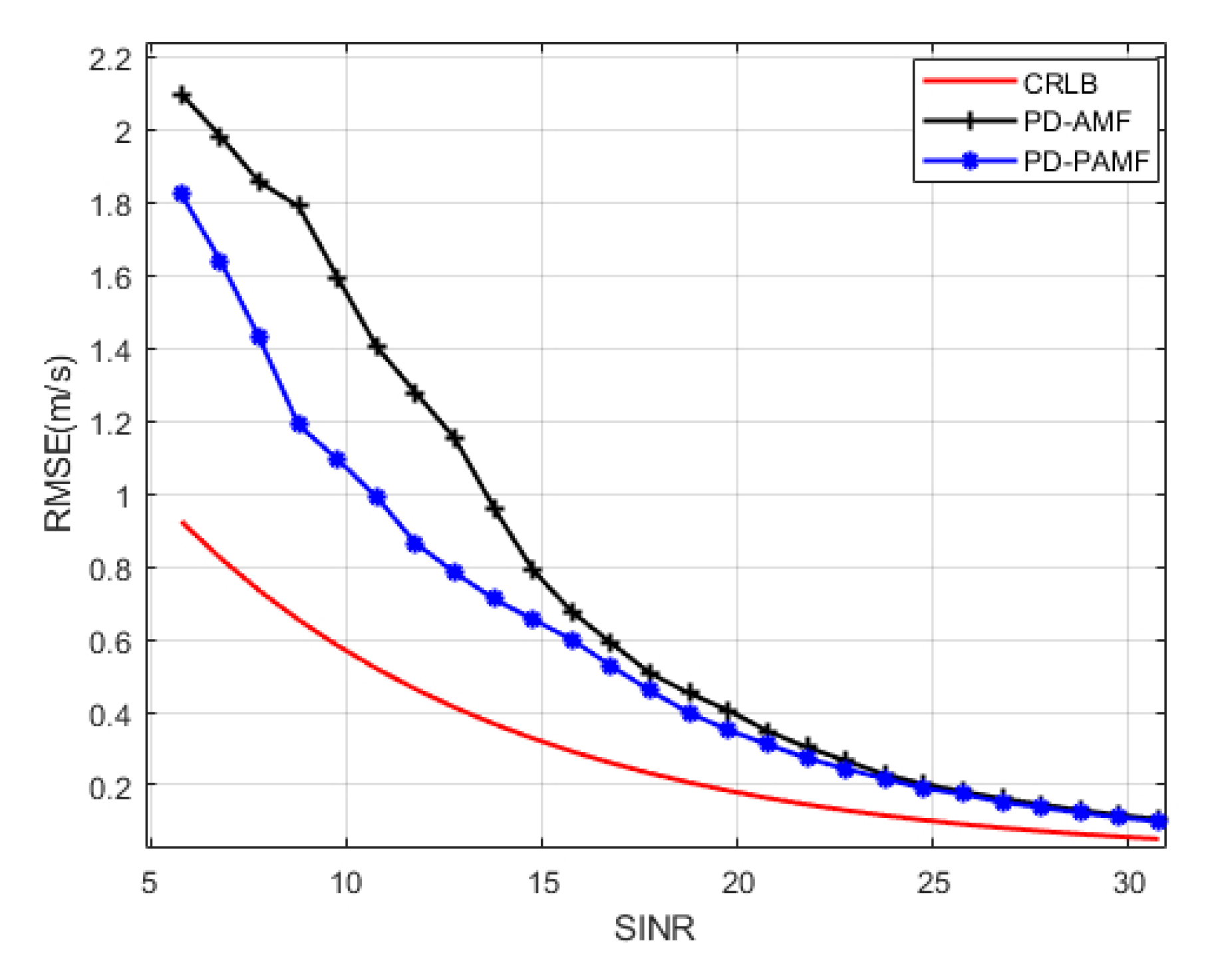
5.1.3. Root Mean Square Error (RMSE) of Velocity versus SINR

Next, we examine the estimation performance of velocity. Velocity is obtained through the maximum likelihood estimation in Equation (33). Figure 5 shows the RMSE of PD-PAMF (blue line) and PD-AMF (black line) with SINR variation. As a reference, we also draw the Cramer Rao Lower Bounds (CRLBs) of the velocity estimation [35]. The results show that, as SINR increases, the RMSE of both detectors decreases, which is closer to CRBL. When SINR < 25 dB, the estimated error of PD-PAMF is smaller than that of PD-AMF. When SINR = 25 dB, the RMSE curves of PD-PAMF and PD-AMF coincide, which is consistent with the results in Figure 4. Therefore, with the support of small samples and low SINR, PD-PAMF has better velocity estimation accuracy, which is closer to the CRBLs.

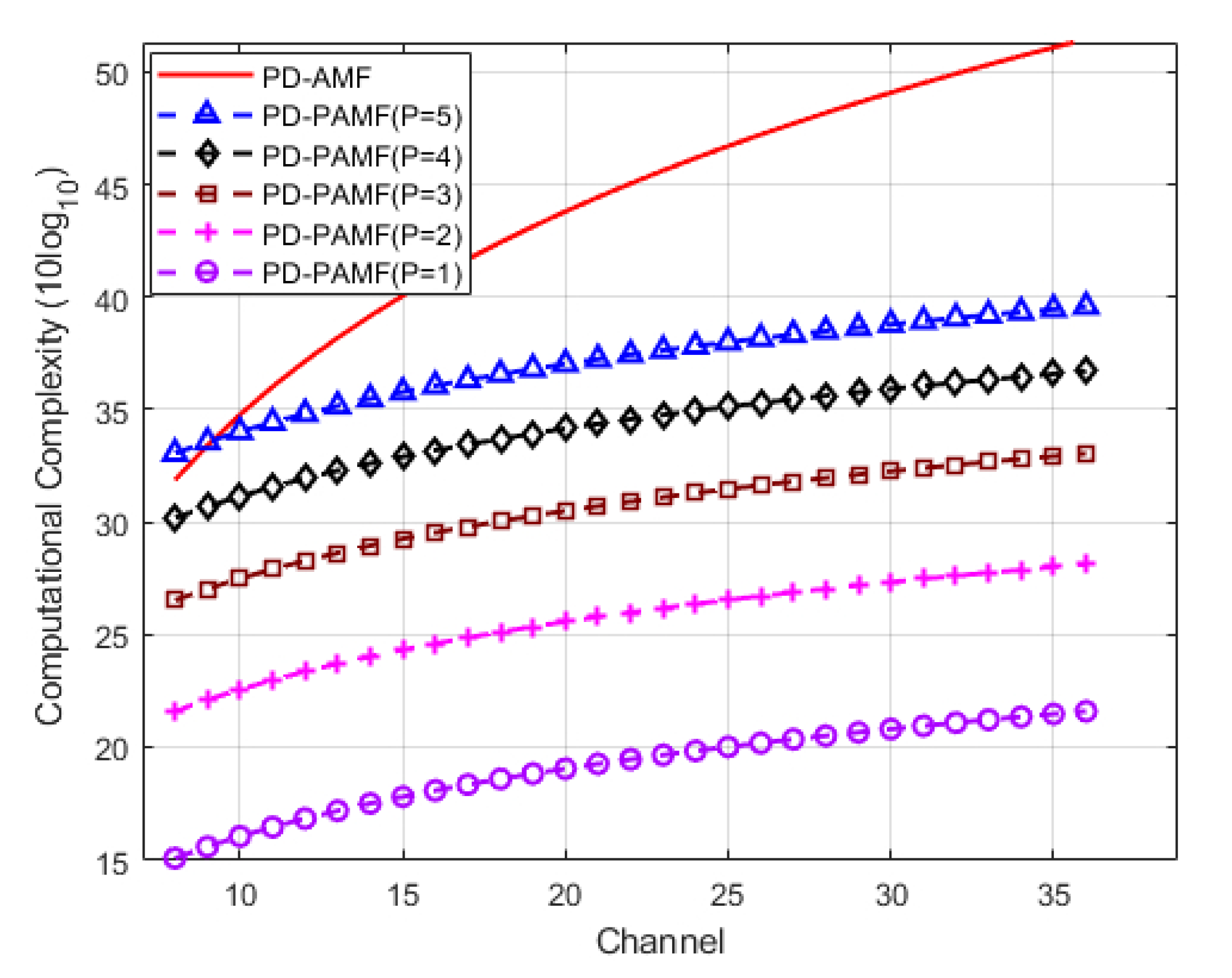
5.1.4. Computational Complexity versus Channels

Lastly, we discuss the computational complexity of the PD-PAMF and the PD-AMF in Figure 6. From Section 4, the computational complexities of PD-PAMF and PD-AM are both related to the training data size K and the number of channels N. In addition, the computational complexity of PD-PAMF is related to the order P of the AR model. Taking into account the number of variables and RMB criteria, this section selects K = 2 N (i.e., RMB requirement), even though PD-PAMF does not require such a large number of samples. The results show that, as the number of radar channels N increases, the computational complexity of PD-AMF increases sharply while the slow increase of PD-PAMF is only caused by the increase in training data K. However, the training data size of the PD-PAMF does not have to follow the RMB requirement because it can achieve higher performance with a small size data. Thus, the proposed PD-PAMF has lower computational complexity.

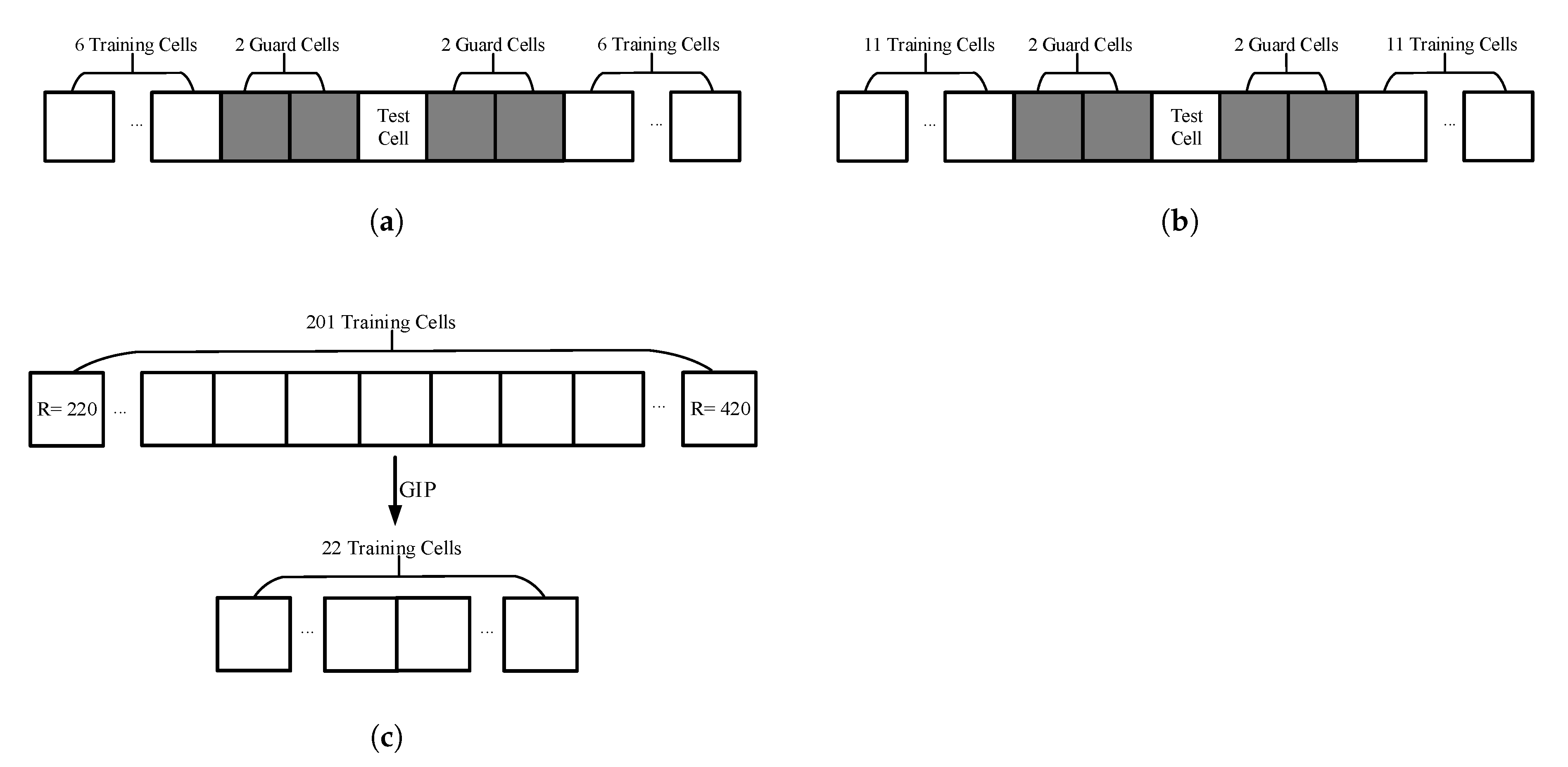
5.2. Detection Performance Using Simulated Airborne Multichannel Radar Data

To demonstrate the effectiveness of the proposed PD-PAMF detector, we further conduct experiments by using the simulated radar data in a dense signal environment. Here, we utilize an airborne synthetic aperture radar (SAR) image scene (as shown in Figure 7, the azimuth is 2000 cells and the range is 800 cells) to simulate the echoes of an airborne array radar with 11 channels via point target simulation (details of the simulation method can be referenced in [36]). Obviously, there are many heterogeneous and strong discrete scatterers in the scene. The system and geometry parameters are shown in

Table 2. System and geometry parameters.

Parameters	Variables	Values
Scene dimensions	Na × Nr	2000 × 800
Wavelength	$\lambda$	0.03 m
Platform velocity	V	100 m/s
Number of channels	N	11
Antenna separation	b	0.1 m
Target direction of arrival	${\theta }_t$	90${}^{\circ }$
Target radial velocity	$v_{rt}$	2 m/s
Pulse repetition frequency	PRF	1000 Hz
Platform Height	Ha	3000 m
Minimum slant range	Rmin	6000 m
Bandwidth	Br	30 MHz
Clutter to noise ratio	CNR	30 dB
Signal to clutter ratio	SCR	2 dB

. Considering that a moving target should remain in one doppler cell during the integration time, 128 pulses and 800 range bins are chosen. The processing CPI is shown in Figure 7, and the yellow rectangle area is the background of clutter when detecting targets in the range-Doppler domain. To evaluate the performance of the PD-PAMF in a dense environment, five injected moving targets are placed in range cells R = 302, 348, 352, 356, and 359. They are all with ${\theta }_t$ = 90${}^{\circ }$, radial velocity $v_{rt}$ = 2 m/s, and Signal to clutter ratio (SCR) = 2 dB (noticing the heterogeneous clutter, we consider local clutter for SCR). The training data containing target signals will sharply degrade the detection performance because of target cancelation by self-whitening. For the problem considered here, we choose the same velocity in order to test the detection performance of the proposed PD-PAMF under more difficult detection conditions. All signals are discrete in range (i.e., each signal occupies only one range cell). It presents a very difficult detection problem under this situation since the signals in the “adjacent cells” that have the same signal steering vector as that in the “test cell” enter the training data used to estimate and reject the disturbance. As a consequence, the “test cell” signal may be self-whitening. Test cell processing occurs in the interval from range cells R = 220–420. In order to research the effects of the training data size and content on the PD-PAMF and the PD-AMF, we consider three test cases. The first test case is to utilize K = 12 training data (small samples) and a moving window consisting of 16 range bins for processing. Four guard range cells are used on the test cell, as shown in Figure 8a. The second test case is to utilize K = 2 N = 22 training data (satisfying RMB rule) and a moving window consisting of 26 range bins for processing, and four range guard cells are used on the test cell, as shown in Figure 8b. The third test case is to use the GIP strategy of training data screening, which eliminates the nonhomogeneous training data containing target signals [10,18]. A fixed window is used. Among the 201 range bins from R = 220 to R = 420, K = 2 N = 22 training data are selected for training, as shown in Figure 8c.

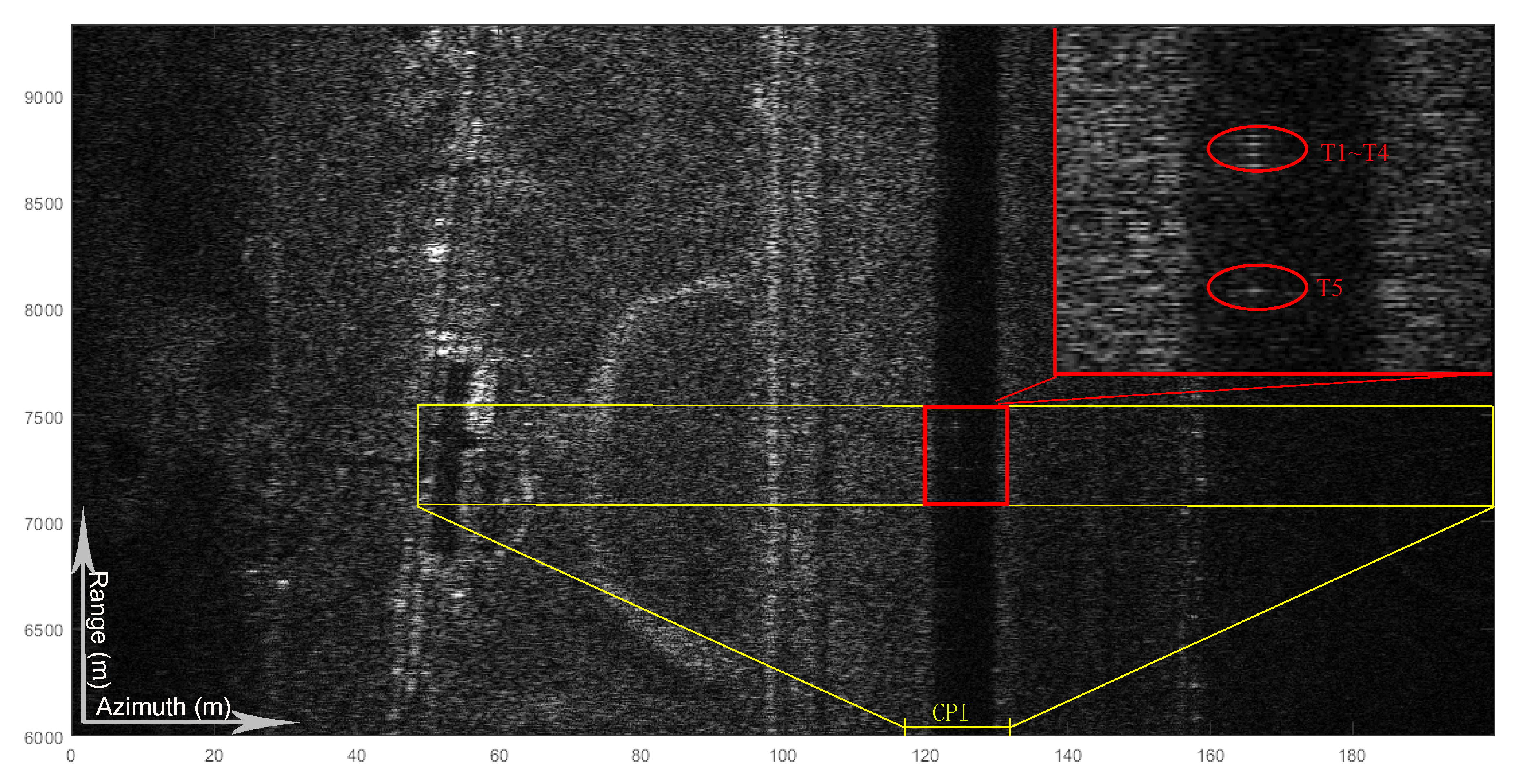
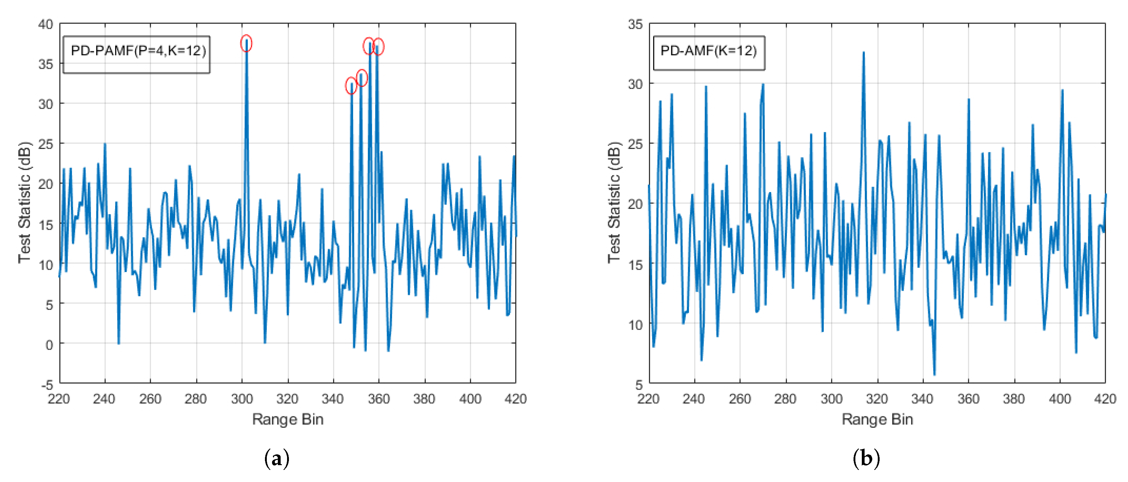
5.2.1. First Test Case

Figure 9a,b show the detection results of the PD-PAMF by using model order P = 4 and the PD-AMF in test case 1, respectively. As we can see, the proposed PD-PAMF accurately detects five moving targets while the PD-AMF does not because of target self-whitening. For the test statistics of the PD-PAMF, the target signals are at least 17 dB above the 15 dB mean value. Additionally, the highest background peak is 8 dB below the lowest target peak. Thus, the PD-PAMF detector outperforms the PD-AMF detector.

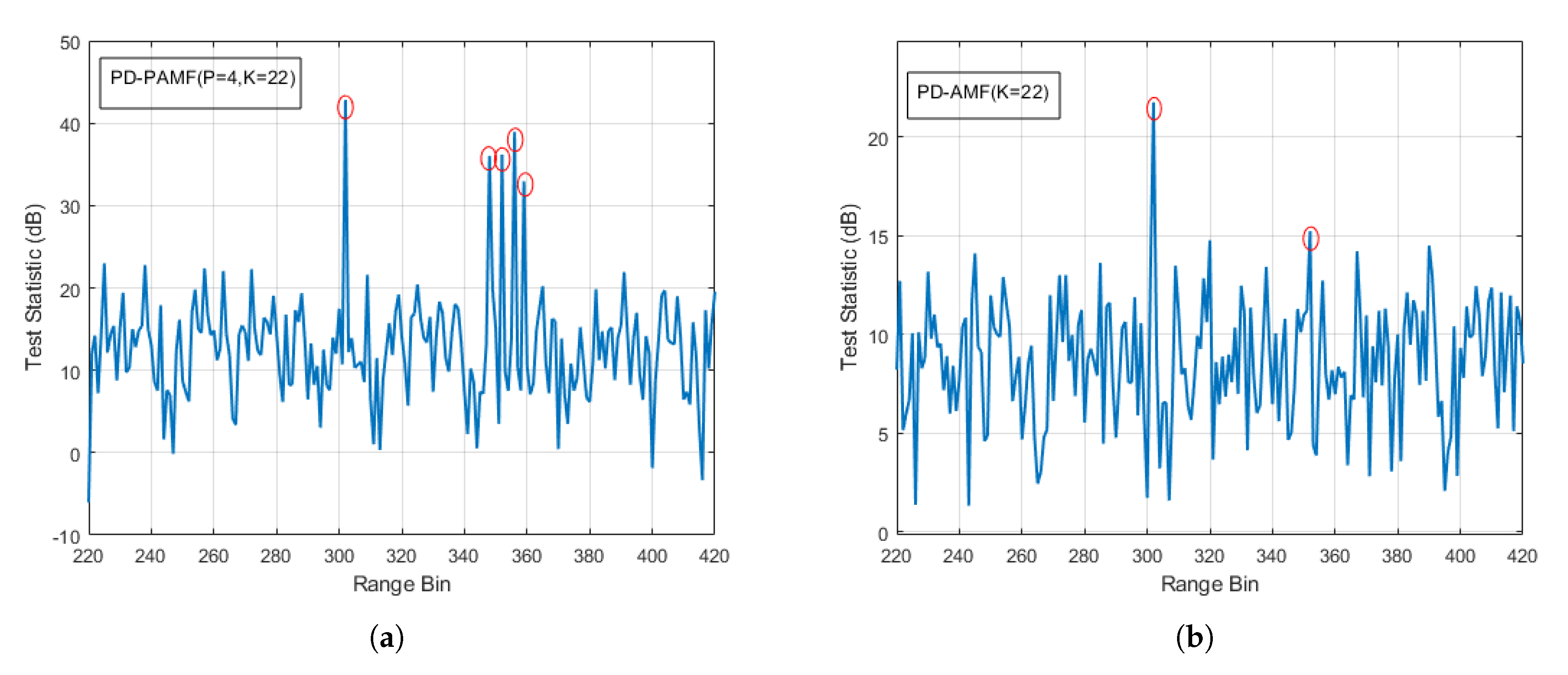
5.2.2. Second Test Case

Figure 10a,b shows the detection results of the PD-PAMF using model order P = 4 and the PD-AMF in test case 2, respectively. The proposed PD-PAMF accurately detects five moving targets, while the PD-AMF detects two. For the test statistics of the PD-PAMF, the target signals are at least 18 dB above the 15 dB mean value. Moreover, the highest background peak is 10 dB below the lowest target peak. For the test statistics of the PD-AMF, the target signals are 7 dB above the 8 dB mean value. However, the highest background peak is close to the lowest target peak. Compared with the PD-AMF, the PD-PAMF improves a lot in detection performance and the processing time of the proposed PD-PAMF reduces by about 1.5 times, which is consitent with the complexity analysis. Thus, the PD-PAMF detector outperforms the PD-AMF detector.

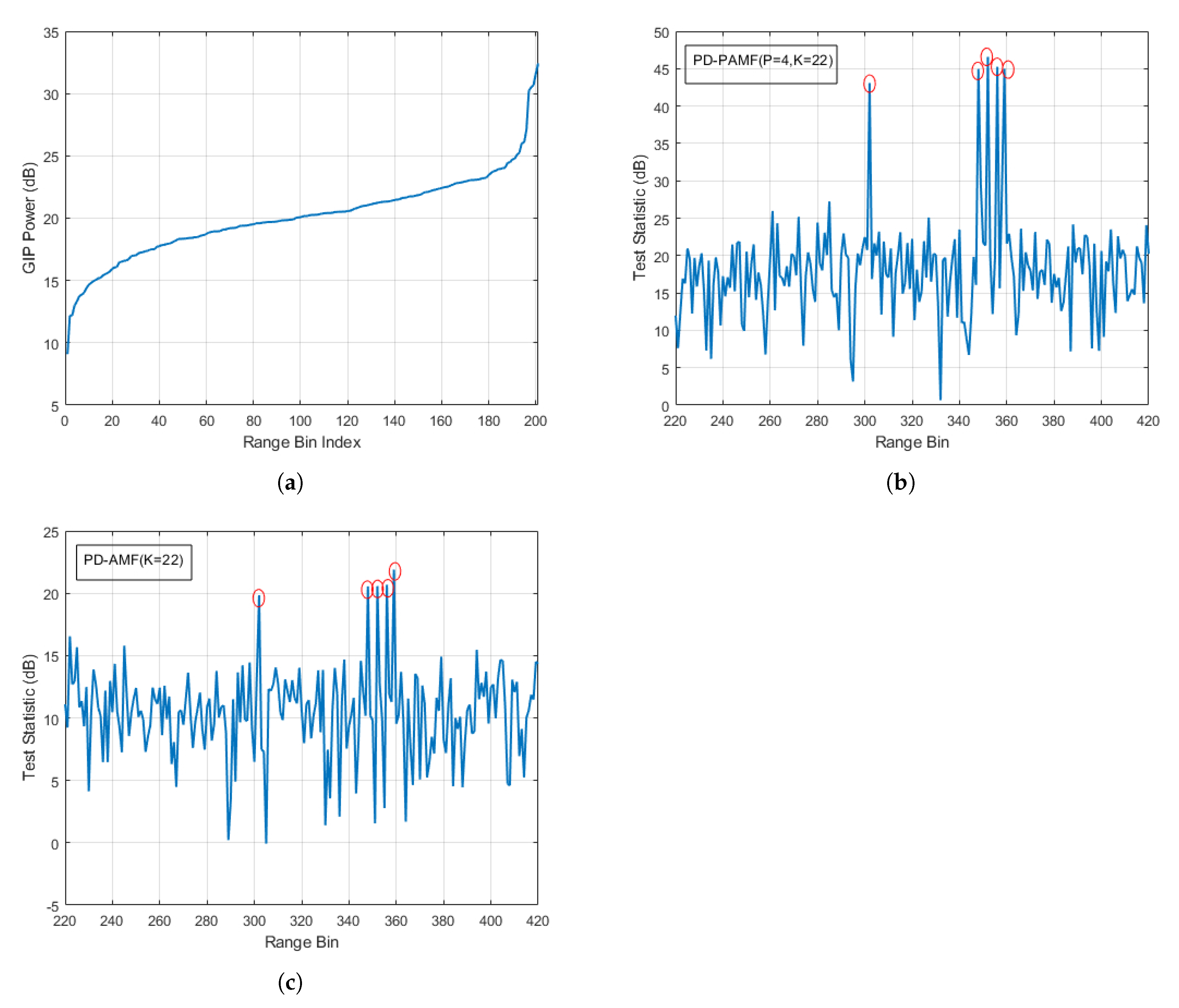
5.2.3. Third Test Case

Figure 11 is the results in test case 3. Figure 11a shows the plots of the sorted GIP value for each range bin. It can be observed that there are many strong scatterers which may include target signals and heterogeneous scatterers. Herein, the first 22 low-power range bins in Figure 11a are selected as training data for the detectors. Figure 11b,c show the detection results of the PD-PAMF using model order P = 4 and the PD-AMF, respectively. Both the proposed PD-PAMF and the PD-AMF accurately detect five moving targets. For the test statistics of the PD-PAMF, the target signals are at least 28 dB above the 15 dB mean value. Additionally, the highest background peak is 16 dB below the lowest target peak. However, compared with the result of Figure 10a, the use of the GIP algorithm only appears to improve the signal strength. For the test statistics of the PD-AMF, the target signals are 9 dB above the 10 dB mean value. However, the highest background peak is only 3 dB below the lowest target peak. Compared with the result in Figure 10b, GIP provides a significant performance improvement for the PD-AMF. It should be pointed out that the use of GIP will greatly increase the computational complexity. Compared with the detector combining PD-AMF with GIP, the processing time of the proposed PD-PAMF reduces by about 6.8 times. Especially, in the real-time application of GMTI radar systems, this is not worthwhile. Thus, the PD-PAMF detector outperforms the PD-AMF detector.

6. Discussion

Herein, we proposed a novel PD-PAMF detector for ground moving target detection. The results suggest a possibility of disturbance suppression by modelling an AR process of low order. In a dense signal environment, the proposed detector offers excellent detection performance while the PD-AMF detector fails to detect the moving targets, which are caused by the training data size and content. Compared with the PD-AMF, the detector combining PD-AMF with GIP can effectively detect targets. However, its processing time increases by about 6.8 times compared with the PD-PAMF, which is not worthwhile in real-time applications.

Compared with previous detectors [5,6,9,21], the proposed PD-PAMF detector has two main characteristics. First, it has lower requirements on the training data size and content in the range-Doppler domain. Even if the training data contain target signals and strong discrete scatters, the detector also shows excellent detection performance. Thus, it can be utilized in a dense signal environment. Second, it does not involve a large matrix inversion and the AR order is also low. Therefore, it is computationally simpler and more suitable for real-time applications.

Although there are important discoveries revealed by these studies, some limitations are also noteworthy. First, the PD-PAMF is based on the AR model for filtering. Therefore, the model cannot fit the disturbance well since the spatial sequence is short (i.e., channels are insufficient); then, the detector may be invalid. Second, the order of the AR model is unknown in practical application. Although there are many methods to determine the order of the AR model [30,31], it may be difficult to estimate in complex radar environments. Further improvement may be possible by adaptively selecting proper model orders for AR processes, which is a topic for future studies. Finally, the proposed PD-PAMF cannot detect targets with only along-track velocities since the phase differences among channels are insensitive to along-track velocities, which is also a common issue for STAP detectors. The issue may be addressed by a time-frequency analysis [37] or a bank of match filters in azimuth [38]. Furthermore, it is meaningful to analyse and evaluate the PD-PAMF performance in different realistic scenarios. Recently, video SAR is a new emerging SAR mode for moving target detection [39]. For the same scene of different frames, the disturbances are also highly relevant. It may be another important research topic in the future.

7. Conclusions

The limitations of training data and computational complexity are two main issues for STAP detectors in an airborne radar. To overcome them, this paper proposes a novel PD-PAMF detector that operates in the range-Doppler domain. Based on the PD-MF and the LDU decomposition of the disturbance covariance matrix, the theory of the PD-PAMF and its mathematical framework are introduced and the versatility of the PD-PAMF is improved by modifying the conventional model of multichannel signal. The key to the novel detector is to model the disturbance of the spatial sequence as an AR process for filtering. The AR coefficients are estimated from the spatial sequence of data for each range cell and further averaged over the K training data cells, which improves the data efficiency. Both PD-PAMF and PD-AMF detectors are examined with small training data size, large training data size, training data containing target signals, and the GIP strategy. The results show that, compared with the well-known PD-AMF technology, PD-PAMF can significantly improve the detection performance with less training data and is more tolerant to strong scatterers and moving target signals contained in the training data. In addition, since it does not involve a large inversion of the covariance matrix, the PD-PAMF also reduces the processing time.

References

1. Brennan, L.E.; Reed, L. Theory of adaptive radar. IEEE Trans. Aerosp. Electron. Syst. 1973, AES-9, 237–252. [Google Scholar] [CrossRef]
2. Reed, I.S.; Mallett, J.D.; Brennan, L.E. Rapid convergence rate in adaptive arrays. IEEE Trans. Aerosp. Electron. Syst. 1974, 6, 853–863. [Google Scholar] [CrossRef]
3. Kelly, E.J. An adaptive detection algorithm. IEEE Trans. Aerosp. Electron. Syst. 1986, AES-22, 115–127. [Google Scholar] [CrossRef] [Green Version]
4. Fuhrmann, D.R.; Kelly, E.J.; Nitzberg, R. A CFAR adaptive matched filter detector. IEEE Trans. Aerosp. Electron. Syst. 1992, 28, 208–216. [Google Scholar]
5. Ward, J. Space-Time Adaptive Processing for Airborne Radar; IEE Colloquium on Space-Time Adaptive Processing: London, UK, 1998. [Google Scholar]
6. Wang, H.; Cai, L. On adaptive spatial-temporal processing for airborne surveillance radar systems. IEEE Aerosp. Electron. Syst. 1994, 30, 660–670. [Google Scholar] [CrossRef]
7. Cerutti-Maori, D.; Klare, J.; Brenner, A.R.; Ender, J.H. Wide-area traffic monitoring with the SAR/GMTI system PAMIR. IEEE Trans. Geosci. Remote Sens. 2008, 46, 3019–3030. [Google Scholar] [CrossRef]
8. Da Silva, A.B.C.; Baumgartner, S.V.; Krieger, G. Training data selection and update strategies for airborne post-doppler stap. IEEE Trans. Geosci. Remote Sens. 2019, 57, 5626–5641. [Google Scholar] [CrossRef] [Green Version]
9. Ender, J.H. Space-time processing for multichannel synthetic aperture radar. Electron. Commun. Eng. J. 1999, 11, 29–38. [Google Scholar] [CrossRef]
10. Gelli, S.; Bacci, A.; Giusti, E.; Martorella, M.; Berizzi, F. Effectiveness of Knowledge-Based STAP in Ground Targets Detection with Real Dataset. In Proceedings of the International Conference on Radar Systems (Radar 2017), Belfast, UK, 23—26 October 2017; pp. 1–5. [Google Scholar] [CrossRef]
11. Rangaswamy, M.; Michels, J.H. A parametric multichannel detection algorithm for correlated non-Gaussian random processes. In Proceedings of the 1997 IEEE National Radar Conference, Syracuse, NY, USA, 13–15 May 1997; pp. 349–354. [Google Scholar]
12. Roman, J.R.; Rangaswamy, M.; Davis, D.W.; Zhang, Q.; Himed, B.; Michels, J.H. Parametric adaptive matched filter for airborne radar applications. IEEE Trans. Aerosp. Electron. Syst. 2000, 36, 677–692. [Google Scholar] [CrossRef]
13. Sohn, K.J.; Li, H.; Himed, B. Parametric Rao test for multichannel adaptive signal detection. IEEE Trans. Aerosp. Electron. Syst. 2007, 43, 921–933. [Google Scholar] [CrossRef]
14. Wang, P.; Li, H.; Himed, B. A new parametric GLRT for multichannel adaptive signal detection. IEEE Trans. Signal Process. 2010, 58, 317–325. [Google Scholar] [CrossRef]
15. Sohn, K.J.; Li, H.; Himed, B. Parametric GLRT for multichannel adaptive signal detection. IEEE Trans. Signal Process. 2007, 55, 5351–5360. [Google Scholar] [CrossRef]
16. Li, H.; Sohn, K.J.; Himed, B. The PAMF Detector is a Parametric Rao Test. In Proceedings of the Conference Record of the Thirty-Ninth Asilomar Conference on Signals, Systems and Computers, Pacific Grove, CA, USA, 30 October–2 November 2005; pp. 1311–1315. [Google Scholar] [CrossRef]
17. Chen, C.W. Performance assessment of along-track interferometry for detecting ground moving targets. In Proceedings of the 2004 IEEE Radar Conference (IEEE Cat. No.04CH37509), Philadelphia, PA, USA, 29 April 2004; pp. 99–104. [Google Scholar] [CrossRef]
18. Michels, J.H.; Himed, B.; Rangaswamy, M. Robust STAP detection in a dense signal airborne radar environment. Signal Process. 2004, 84, 1625–1636. [Google Scholar] [CrossRef]
19. Alfano, G.; De Maio, A.; Farina, A. Model-based adaptive detection of range-spread targets. IEEE Proc. Radar Sonar Navig. 2004, 151, 2–10. [Google Scholar] [CrossRef]
20. Melvin, W.L. A stap overview. IEEE Aerosp. Electron. Syst. Mag. 2004, 19, 19–35. [Google Scholar] [CrossRef]
21. Cerutti-Maori, D.; Sikaneta, I. A generalization of DPCA processing for multichannel SAR/GMTI radars. IEEE Trans. Geosci. Remote Sens. 2012, 51, 560–572. [Google Scholar] [CrossRef]
22. Kirk, J. Motion Compensation for Synthetic Aperture Radar. IEEE Trans. Aerosp. Electron. Syst. 1975, AES-11, 338–348. [Google Scholar] [CrossRef]
23. Zeng, L.; Liang, Y.; Xing, M.; Huai, Y.; Li, Z. A Novel Motion Compensation Approach for Airborne Spotlight SAR of High-Resolution and High-Squint Mode. IEEE Geosci. Remote Sens. Lett. 2016, 13, 429–433. [Google Scholar] [CrossRef]
24. Da Silva, A.B.C.; Baumgartner, S.V.; de Almeida, F.Q.; Krieger, G. In-Flight Multichannel Calibration for Along-Track Interferometric Airborne Radar. IEEE Trans. Geosci. Remote. Sens. 2020, 1–18. [Google Scholar] [CrossRef]
25. Gierull, C.H. Moving Target Detection with Along-Track SAR Interferometry; Technical Report 2002-084; Technical memorandum; Defence R & D Canada-Ottawa: Ottawa, ON, Canada, 2002. [Google Scholar]
26. Gierull, C.; Ottawa, D.R.D.C. Digital Channel Balancing of Along-Track Interferometric SAR Data; Technical memorandum; Defence R & D Canada-Ottawa: Ottawa, ON, Canada, 2003. [Google Scholar]
27. Therrien, C. On the relation between triangular matrix decomposition and linear prediction. Proc. IEEE 1983, 71, 1459–1460. [Google Scholar] [CrossRef]
28. Haykin, S. Adaptive Radar Detection and Estimation; WILEY-INTERSCIENCE: Hoboken, NJ, USA, 1992. [Google Scholar]
29. Akaike, H. A new look at the statistical model identification. IEEE Trans. Autom. Control 1974, 19, 716–723. [Google Scholar] [CrossRef]
30. Rissanen, J. Modeling by shortest data description. Automatica 1978, 14, 465–471. [Google Scholar] [CrossRef]
31. Marple, S.L., Jr.; Carey, W.M. Digital Spectral Analysis with Applications. J. Acounsti. Soc. Am. 1989, 86, 2043. [Google Scholar] [CrossRef] [Green Version]
32. Michels, J.; Himed, B.; Rangaswamy, M. Evaluation of the normalized parametric adaptive matched filter STAP test in airborne radar clutter. In Proceedings of the Record of the IEEE 2000 International Radar Conference [Cat. No. 00CH37037], Alexandria, VA, USA, 12 May 2000; pp. 769–774. [Google Scholar] [CrossRef]
33. Michels, J.H.; Rangaswamy, M.; Himed, B. Performance of parametric and covariance based STAP tests in compound-Gaussian clutter. Digit. Signal Process. 2002, 12, 307–328. [Google Scholar] [CrossRef]
34. Wang, P.; Li, H.; Himed, B. A parametric moving target detector for distributed MIMO radar in non-homogeneous environment. IEEE Trans. Signal Process. 2013, 61, 2282–2294. [Google Scholar] [CrossRef]
35. Ender, J.H.; Gierull, C.H.; Cerutti-Maori, D. Improved space-based moving target indication via alternate transmission and receiver switching. IEEE Trans. Geosci. Remote Sens. 2008, 46, 3960–3974. [Google Scholar] [CrossRef]
36. Allan, J.M.; Collins, M.J.; Gierull, C. Computational synthetic aperture radar (cSAR): A flexible signal simulator for multichannel SAR systems. Can. J. Remote Sens. 2010, 36, 345–360. [Google Scholar] [CrossRef]
37. Barbarossa, S.; Farina, A. Detection and imaging of moving objects with synthetic aperture radar. 2. Joint time-frequency analysis by Wigner-Ville distribution. Radar Signal Process. IEEE Proc. F 1992, 139, 79–88. [Google Scholar] [CrossRef]
38. Cristallini, D.; Pastina, D.; Colone, F.; Lombardo, P. Efficient Detection and Imaging of Moving Targets in SAR Images Based on Chirp Scaling. IEEE Trans. Geoence Remote Sens. 2013, 51, 2403–2416. [Google Scholar] [CrossRef]
39. Pu, W.; Wang, X.; Wu, J.; Huang, Y.; Yang, J. Video SAR Imaging Based on Low-Rank Tensor Recovery. IEEE Trans. Neural Networks Learn. Syst. 2020, 1–15. [Google Scholar] [CrossRef]
Figure 1. Acquisition geometry using a multichannel antenna.
Remotesensing 12 04017 g001
Figure 2. Post-Doppler parametric adaptive matched filter (PD-PAMF) detection architecture.
Remotesensing 12 04017 g002
Figure 3. Receiver Operating Characteristic (ROC) curves (a) AR(5), K = 2 N = 22; (b) AR(3), K = 11; and (c) one target in training data, PD-PAMF: AR(5), K = 11, PD-AMF: K = 2 N = 22.
Remotesensing 12 04017 g003
Figure 4. Probability of Detection versus SINR, AR(3), P F A = 10 2 , K = 11.
Remotesensing 12 04017 g004
Figure 5. Root Mean Square Error (RMSE) of velocity versus signal-to-interference-and-noise ratio (SINR), AR(3), P F A = 10 2 , K = 11.
Remotesensing 12 04017 g005
Figure 6. Computational complexity versus channels, K = 2 N, AR(1), AR(2), AR(3), AR(4), AR(5).
Remotesensing 12 04017 g006
Figure 7. SAR scene with five injected targets.
Remotesensing 12 04017 g007
Figure 8. Training data selection: (a) first test case, (b) second test case, and (c) third test case.
Remotesensing 12 04017 g008
Figure 9. Detection results with K = 11 and a moving window and a target signal (red circle): (a) PD-PAMF test statistics, AR(4), five targets in R = 302, 348, 352, 356, and 359 and (b) PD-AMF test statistics, no targets.
Remotesensing 12 04017 g009
Figure 10. Detection results with K = 2N = 22 and moving windows and a target signal (red circle): (a) PD-PAMF test statistics, AR(4), five targets in R = 302, 348, 352, 356, and 359 and (b) PD-AMF test statistics, two targets in R = 302 and 352.
Remotesensing 12 04017 g010
Figure 11. Detection results of the generalized inner product (GIP) with K = 2N = 22 and fixed windows and a target signal (red circle): (a) sorted GIP power; (b) PD-PAMF test statistic, AR(4), five targets in R = 302, 348, 352, 356, 356, and 359; and (c) PD-AMF test statistics, five targets in R = 302, 348, 352, 356, and 359.
Remotesensing 12 04017 g011