Quantification and Mapping of Satellite Driven Surface Energy Balance Fluxes in Semi-Arid to Arid Inter-Mountain Region

Abstract

Crop evapotranspiration (ET_c) estimates, on a regional scale, hold enormous potential in managing surface and groundwater resources. This is particularly important for the headwater state of Wyoming, which provides water to found major river basins of the US. In this study, METRIC (Mapping evapotranspiration at high resolution with internalized calibration), a satellite-based image processing model, was used to map and quantify daily, monthly, and seasonal ET_c and other energy balance fluxes, i.e., net radiation (R_n), sensible heat (H), and soil heat flux (G) dynamics for different land-use classes. Monthly and seasonal ETc estimated were further used to approximate regional water consumption patterns for different land-use types for nine irrigation districts in semi-arid to arid intermountain region of Big Horn Basin (BHB), Wyoming. The validation of METRIC retrievals against Bowen ratio energy balance system (BREBS) fluxes measured over three vegetative surfaces, viz. sugar beet in 2017, dry bean in 2018, and barley in 2019, indicated high accuracy. The pooled correlation observed between estimated (pooled) and measured instantaneous fluxes had R² values of 0.91 (RMSE = 0.08 mm h⁻¹, NSE = 0.91), 0.81 (RMSE = 49.6 Wm⁻², NSE = 0.67), 0.53 (RMSE = 27.1 Wm⁻², NSE = 0.53), and 0.86 (RMSE = 59.2 Wm⁻², NSE = 0.84) for ET_c, R_n, G, and H, respectively. The biggest discrepancy between measured and estimated monthly ETc values was observed during times when BREBS flux tower footprint was devoid of any crops or the crops at footprint were not actively transpiring. Validation results improved when comparisons were made on monthly scales with METRIC underestimating growing season ET_c in the range between 3.2% to 6.0%. Seasonal ETc by land-use type showed significant variation over the study area where crop ETc was 52% higher than natural vegetation ETc. Furthermore, it was found that, in the arid to semi-arid intermountain region of Wyoming, the contribution of irrigation to total seasonal ETc varied in the range of 73–81% in nine irrigation districts that fall within the study area. The high relative contribution of irrigation highlights the importance of identifying and quantifying ETc for improved management in irrigation system design and water allocation.

1. Introduction

The availability of freshwater resources for agroecosystems has been an important issue for the sustainability of agricultural production in the U.S. and around the world. This is particularly important to the arid to semi-arid regions of the western U.S.A, including Wyoming, where climatic variability, drought, and water scarcity are becoming a persistent challenge [1]. In the inter-mountain region of Wyoming, irrigated agriculture is the backbone of the state’s economy, representing an annual income of approximately $1.8 billion [2]. Irrigated agriculture accounts for 80–85% of total consumptive water use, with the state irrigating approximately 0.60–0.65 million hectares annually depending upon the surface and groundwater supplies. As Wyoming’s agricultural, municipal, industrial, and recreational/environmental water uses increase, the state’s limited water supplies have come under increased scrutiny. This has led to the scrutiny of surface and groundwater by the state and local governments, leading to the development of new regulatory approaches and groundwater policies. Although the Wyoming State Constitution decrees that all water inside its boundaries is the property of the state, several interstate water compacts and court decrees limit the amount of outgoing streamflow that Wyoming can deplete [3]. Wyoming is also a headwater state and provides water to four major river basins of the US. Wyoming’s land area drains into the Missouri-Mississippi River basin (approximately 72%), Green-Colorado River Basin (approximately 17%), Snake-Columbia River Basin (approximately 5%), and Great Salt Lake Basin (approximately 2%) [4]. Interstate compacts and decrees between upstream and downstream user states have placed some restrictions on the amount of streamflow Wyoming users can deplete. Under these circumstances, the management of water resources at the field, watershed, and regional scales is critical to sustained crop production and economic vitality in the region’s agro-ecosystem.

The efficient use of water resources in agriculture and to understand the response of agro-ecosystems to changing environment require the adequate quantification of crop evapotranspiration (ET_c; latent heat flux) and other surface energy balance fluxes (net radiation (R_n), soil heat flux (G), and sensible heat flux (H)) on both point and regional scales. ET_c, a combination of evaporation and transpiration fluxes, is an important component of the agro-ecosystem and plays a significant role in determining the mass and energy transfer between the hydrosphere, atmosphere, and biosphere by impacting the relationships between land-use/land cover change and microclimate/climate energy balance in the hydrologic cycle [5,6,7,8]. In agricultural settings, ET_c is directly related to plant biomass and contributes to the determination of crop irrigation water requirements, groundwater consumption, water allocation in a river basin, irrigation reservoirs, storage and conveyance system capacities, and water rights [9,10].

Although highly established and localized techniques, such as eddy covariance [11], Bowen ratio energy balance [5], lysimeter [12], etc., have been widely used for the continuous measurement of ET_c, their application beyond the local scale (watershed/regional scale) has become challenging because of the high cost of instrumentation, complexity, and effectiveness of the measurement. In general, the footprint of ET_c measurement by these methods is relatively smaller, which creates a significant bias at watershed/regional scales due to heterogeneity of the land surface and the complex nature of the heat transfer process governing the ET_c [13,14]. Another popular and easy method used to quantify crop ET_c is by adjusting the reference (potential) evapotranspiration (ET_r) with crop coefficients (K_c) using the Food and Agricultural Organisation (FAO) Irrigation and Drainage paper number 56 approach [10]. However, this approach over a regional scale does not consider the within-season spatial variation in crop growth stages (even for the same crop), management practices (irrigation, fertilization, etc), soil type, local climate variation, etc. increasing uncertainties in results [8]. Remote sensing-based estimation of ET_c using freely available satellite data in conjunction with meteorological data via surface energy balance techniques can provide the viable means to map-regional patterns of surface energy balance fluxes both spatially and temporally in a consistent and economically practical manner. Over time, different surface energy balance-based algorithms with varying complexities have been developed to quantify spatial and temporal dynamics of energy balance fluxes, e.g., surface energy balance algorithm for land (SEBAL) model [15], surface energy balance system (SEBS) model [14], surface energy balance index (SEBI) model [16], simplified surface energy balance index (S-SEBI) model [17], operational simplified surface energy balance (SSEBop) model [18], mapping evapotranspiration at a high-resolution with internalized calibration (METRIC) model [19], etc. All these models utilize multispectral data from visible and thermal sensors onboard different satellites to identify the differences in land surface characteristics and to estimate ET_c.

In this study, METRIC (mapping evapotranspiration at high resolution using internalized calibration), a satellite-based surface energy balance algorithm formulated by Allen et al. [19,20], based on the (surface energy balance algorithm for land) SEBAL model [15,21,22,23,24], was used to evaluate ET_c and other energy balance flux, viz. Rn, H, and G. Allen et al. [19] report the accuracy of METRIC to be heavily dependent upon choosing appropriate hot and cold pixel points (anchor pixels) within a given image during the calibration process, also know as calibration using inverse modeling at extreme conditions (CIMES). In this process, it uses an internal calibration procedure to estimate the near-surface temperature gradient (dT function) as an indexed function of radiometric surface temperature (Ts) for estimating the H component of the surface energy balance. This procedure further eliminates the need for atmospheric correction of Ts and albedo. Generally, a cold pixel is a well-irrigated field with full crop cover, transpiring actively and a dry pixel is a dry field with approximately zero ET_c. The selection of these extreme pixels is extremely important and requires careful consideration of maps of Ts, normalized difference vegetative index (NDVI), leaf ares index (LAI), surface albedo, land use, and image in true and false colors. Moreover, this procedure uses the hourly reference evapotranspiration (ET_r) to auto-calibrate the H calculation for each satellite image, which makes ET_c estimates more robust [20,25].

Since its introduction, METRIC has been applied worldwide to evaluate and estimate spatial and temporal variability of ET_c under different vegetative and climatic conditions at different spatial and temporal scales. In the US, METRIC has been extensively used to manage water use in cropland, riparian and forest vegetation [19,26,27,28,29,30], regulate water allocation in a river basin and water rights [9], and regulate groundwater withdrawal [31]. Outside the U.S., METRIC has been applied to several regions of the world [26,29,32,33]. For example, Allen et.al. [19] applied METRIC with Landsat images in Idaho, US to predict monthly and season ETc and reported the difference between METRIC estimated and lysimeter measured growing season ET_c to be less than 5%. They further used METRIC monthly and seasonal regional ETc estimates to quantify the net ground-water pumpage and total depletion of water from Bear River systems and Snake River aquifer systems to regulate water rights [9]. Likewise, Singh & Senay [34] tested the METRIC model using Landsat images over three Ameriflux cropland sites in the Mid-western United States. The daily ET_c from three flux sites had an average R² of 0.92 and an average RMSE of 0.93 mm d⁻¹. Singh et al. [35] used the METRIC model in conjunction with the wet METRIC (a modified version of METRIC) model for analyzing Landsat images in the mid-western United States. They reported that the model-estimated daily ET_c was in good agreement with eddy covariance measurements with an average R² of 0.91 and a standard error of 0.6 mm day⁻¹. Furthermore, Mokhtari et al. [36] reported that monthly ET_c estimated using the METRIC model falls within ±10% of the actual ET_c. Tang et al. [37] concluded that METRIC estimated instantaneous and daily ET_c values fall within 10–15% of the actual ET_c. They also mentioned that METRIC estimated seasonal ET_c was overestimated as compared to that of flux measurements. The METRIC model also showed a promising result in the study conducted on apple and olive orchards [38,39,40].

Unlike its applications over flat cropland areas, only limited studies have been focused on its application to mountainous terrain where there is significant relief and a wide range of slopes and aspects. Thus, a local modification of the algorithms is required. This includes the adjustment of the solar and thermal radiation estimates for slope, aspect, and elevation. Moreover, wind speed and aerodynamic roughness are adjusted to account for the impacts of drag due to undulating topography [19,33,41]. Therefore, the main goals of this study were: to (i) assess the performance of the METRIC algorithm to estimate ET_c and other energy balance fluxes using Landsat imagery with respect to measured surface energy balance variables from Bowen ratio energy balance system for the different vegetative surface in the intermountain region of Wyoming; (ii) quantify, map, and evaluate spatial and temporal distribution (daily, monthly and seasonal) of ET_c and other energy balance fluxes over the study region; and (iii) quantify the seasonal crop water use and percent contribution of irrigation toward ET_c for different vegetative surfaces and different irrigation districts within the study area.

2. Materials and Methods

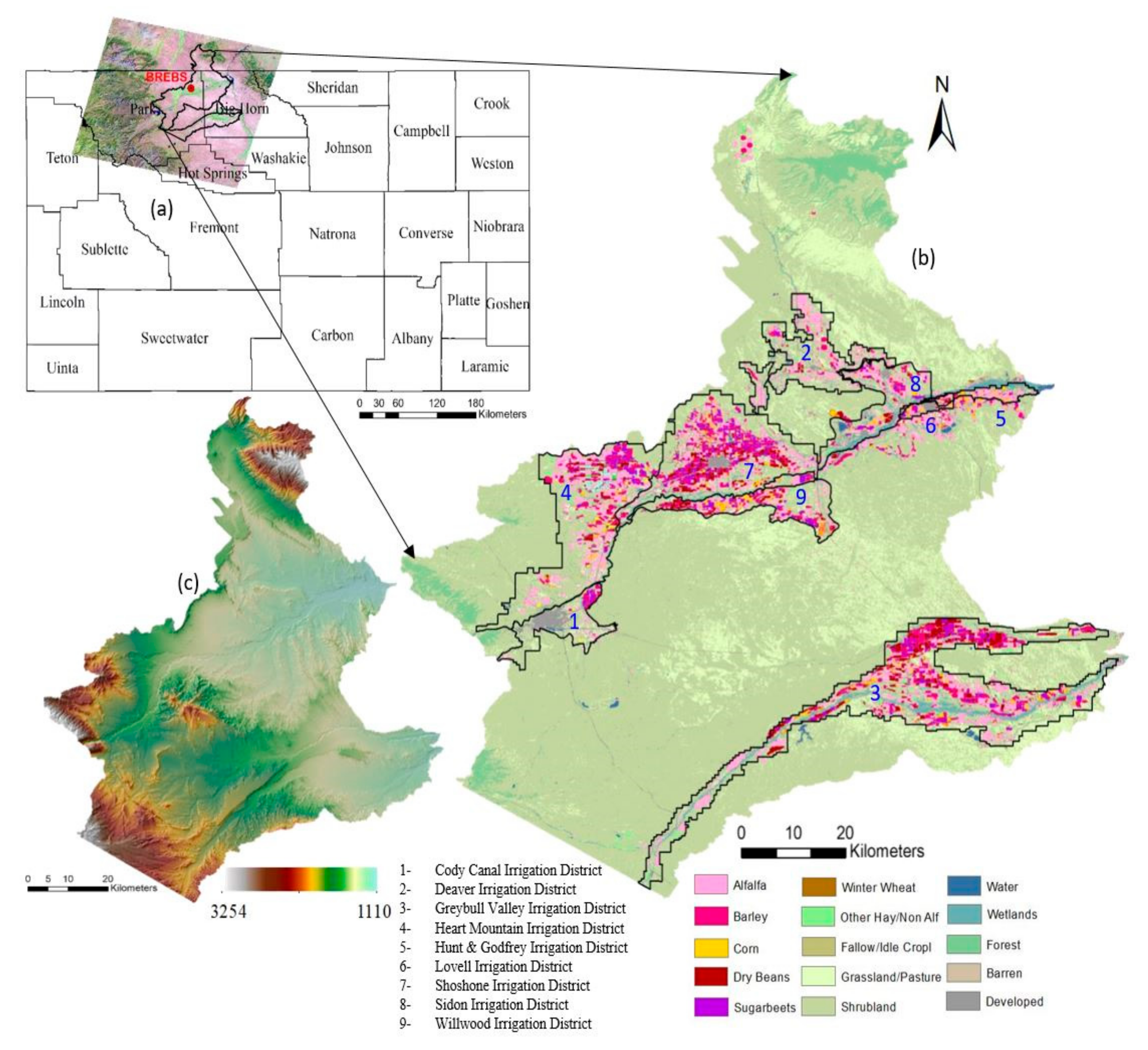
2.1. Study Area

The study area covers the arid to semi-arid region of the Big Horn Basin (BHB), Wyoming which lies in the coverage of Landsat Path: 37 and Row: 29 centered at 44.40°N, 108.52°W (Figure 1). Situated in the Rocky Mountain region of the Western United States, the BHB is dominated by mountain ranges and high elevation plains and covers the highly developed irrigation-based agricultural system within nine irrigation districts which are fed by three major rivers in the regions, namely the Shoshone River, Big Horn River, and Greybull River (Figure 1). The surface elevation of the study region varies from 1110 m to 3254 m above mean sea level. The major soil type in the study area is sandy loam, with a total study area of 7930 km². Annual average P over the study region can vary from over 639 mm in the high elevation mountainous regions to as low as 142 mm in the lower elevation agricultural plains, with an average of 235 mm compared to the state and national average (Contiguous US) of 406 and 762 mm, respectively [42].

In the inter-mountain region of Wyoming, the growing season is generally short due to a limited number of frost-free days in the year. Despite the limited season, the region provides an ideal environment to grow high-yielding and high-quality crops. Natural vegetation covers about 83% of our study area whereas the cropland area is limited to about 14%. Alfalfa is the major crop grown in terms of total acreage, followed by barley, sugar beet, dry bean, and maize, primarily under furrow irrigation with many growers switching to center pivot irrigation [43]. The growing season in the study area starts with the sowing of barley beginning mid-March, sugar beet in Mid April, maize and dry bean in mid to late May, and ends with harvesting that usually starts from August for barley, early September for dry bean, mid to late September for sugar beet until mid-November for Maize. Because of relatively low growing season precipitation (P) and low relative humidity (RH), disease incidence is minimal, and cool winter temperatures suppress insect and disease cycles and much acreage of the region is dedicated to producing certified seed, including dry beans. The natural vegetation comprises evergreen and deciduous forest, grassland, shrubland, and woody and herbaceous wetlands (Figure 1).

High-quality hourly and daily weather data including maximum and minimum air temperature (T_max and T_min), maximum and minimum relative humidity (RH_max and RH_min), wind speed at 2-m height (u₂), incoming solar radiation (Rs), and precipitation (P) were collected from the Wyoming Agricultural Climate Network (WACNet) weather station at the University of Wyoming Powell Research and Extension Center (PREC), located within the Landsat scene footprint [43]. The measured weather data were used to estimate alfalfa reference ET (ET_r), which is utilized in METRIC algorithm to internally calibrate (hourly ET_r) and upscale (daily ET_r) instantaneous ET_c to daily and periodic ET_c. Daily precipitation data are helpful to estimate bare soil evaporation and evaluate prior Landsat image-acquisition date precipitation. The ground-based windspeed values are used to calculate wind speed at blending height (200 m) needed during H calculation. Air temperature and RH values are utilized to calculate dew point temperature (T_dew) and vapor pressure which is then used to compute atmospheric transmissivity. Atmospheric transmissivity signifies the ability of Earth’s atmosphere to allow/pass incoming radiation from the sun and is required during calculation of R_n.

Table 1. Image acquisition date, spacecraft ID, and daily weather parameters measured at BREBS station, Powell Research and Extension Center, Wyoming. Daily weather parameters include minimum air temperature (T_min), maximum air temperature (T_max), minimum relative humidity (RH_min), maximum relative humidity (RH_max), wind speed (u₂), solar radiation (R_s), precipitation (P), and ASCE PM alfalfa-reference evapotranspiration (ETr).

Date	ID	Julian Date	Tmin (°C)	Tmax (°C)	RHmin (%)	RHmax (%)	u2 (ms−1)	Rs (W m−2)	P (mm)	ETr (mm d−1)
4 May 2017	L07	124	1.4	17.7	22.9	84.8	2.0	324.0	0	5.47
5 June 2017	L07	156	12.2	32.7	11.2	65.3	2.0	336.0	0	9.23
21 June 2017	L07	172	10.8	31.4	19.0	80.0	2.1	268.4	0.254	7.95
15 July 2017	L08	196	15.9	36.8	13.0	66.2	1.2	280.1	0	7.28
31 July 2017	L08	212	10.8	33.3	12.4	84.3	0.9	306.0	0	6.3
16 August 2017	L08	228	9.7	25.3	22.6	82.6	0.8	217.8	0	4.14
1 September 2017	L08	244	15.0	31.4	17.6	68.4	1.2	178.3	0	5.15
9 September 2017	L07	252	8.1	30.2	11.6	65.6	0.8	198.2	0	4.25
15 May 2018	L08	135	6.2	19.9	33.8	100	1.4	235.9	0	4.33
8 June 2018	L07	159	10.7	27.0	24.6	82.1	1.4	230.4	0	5.55
2 July 2018	L08	183	10.4	27.8	16.2	81.7	0.8	300.0	0	5.55
18 July 2018	L08	199	11.8	29.5	23.6	84.0	0.7	210.6	0.254	4.55
26 July 2018	L07	207	14.6	28.8	26.8	69.6	1.5	262.7	0	6.36
11 August 2018	L07	223	12.4	36.4	9.0	68.2	0.7	302.5	0	5.95
4 September 2018	L08	247	6.8	30.7	11.6	77.8	1.3	261.8	0	6.03
12 September 2018	L07	255	8.7	24.7	18.1	69.6	1.0	207.3	0	4.12
22 October 2018	L08	295	−0.2	21.6	16.8	74.0	0.9	151.5	0	2.49
3 June 2019	L08	154	8.9	27.3	20.3	84.4	1.1	301.2	0	5.97
13 July 2019	L07	194	13.3	33.4	20.8	82.5	0.9	300.5	0	6.26
21 July 2019	L08	202	12.0	27.5	21.8	57	1.9	332.8	0	7.63
14 August 2019	L07	226	9.5	28.3	19.4	77.8	1.2	298.5	0	6.01
15 September 2019	L07	258	8.6	29.1	13.9	80.7	1.9	192.3	0	5.99

outlines the average meteorological conditions at PREC on the Landsat image acquisition date.

Assessing the uncertainties in satellite estimated ETc using a ground-based measured ETc is an important and challenging task. While the objective of this study is to assess the performance of METRIC estimated ETc for the complex mountainous terrain, however, no ground-measured fluxes were available for those areas. In this study, the accuracy of METRIC estimated surface energy balance fluxes were assessed using the field measured dataset for different vegetation from Bowen ratio energy balance system (BREBS) located at the center of the study area at PREC (44.46°N, 108.45°W) in a large center pivot irrigation production field (14 ha) with a fetch distance of 180 m, 230 m, 223 m, and 160 m in the north, east, south, and west directions, respectively (Figure 2). The BREBS station was installed on a center-pivot field in June 2017 and continuously sampled the energy flux components and other microclimate variables every 60 s and averaged over 15-mi scales during both crop growing and non-growing seasons using a CR10X datalogger and AM416 relay multiplexer (Campbell Scientific, Inc., Logan, Utah). The BREBS measures ET as latent heat (LE; also known as ET_c) based on the energy balance equation as:

$$\mathrm{LE}= \frac{{\mathrm{R}}_{\mathrm{n}}-\mathrm{G}}{1+\mathsf{\beta }}$$

(1)

where β a is the Bowen ratio, which is defined as the ratio of sensible heat flux to latent heat flux [44]. The Bowen ratio is calculated from the differences in air temperature (T_air) and vapor pressure measured at two heights above the crop canopy. The systems measure T_air and RH using two platinum resistance thermometers and monolithic capacitive humidity sensors (REBS models THP04015 and THP04016, respectively) with resolutions of 0.0055 °C for temperature and 0.033% for relative humidity. The T_air and RH sensors are located at the center of two coaxial anodized aluminum radiation shield at two heights. It is important to note that a small bias in temperature and relative humidity measurements can cause incorrect estimation of gradients which can cause significant error in β and LE. Therefore, to minimize the impact of any bias, the system automatically exchanges the temperature and humidity sensors every 15 min at two heights above the canopy. Additionally, aluminum housing units for T_air and RH sensors face the north direction to avoid any impact of direct sunlight on T_air and RH measurements. The system is designed to measure all the components of radiation balance, i.e., incoming and outgoing shortwave and longwave radiation, from which R_n is calculated. The R_n is measured using a REBS Q*7.1 net radiometer that is installed 3 m above the crop canopy using the tripod assembly. To eliminate the effect of reflection of heat and radiation other instruments installed on the tripod and to capture the R_n at the vegetation surface all the R_n measurements are taken away from the tripod station. Other radiation balance components, i.e., incoming and outgoing shortwave and longwave radiation are measured using the REBS models THRDS7.1 double-sided total hemispherical radiometer. The P is recorded using a model TR-525 tipping bucket rain gauge with 0.1 mm resolution. Wind speed and direction above the canopy at 3 m height are measured using a model 034B cup anemometer. The G is measured using three REBS HFT-3.1 heat flux plates and three soil thermocouples installed in close proximity, 0.06 m below the soil surface under the net radiometer assembly. One soil temperature and one SMP1R surface soil moisture sensor were also installed nearby of heat flux plated to G correction. Detailed information on BREBS functioning and instrumentation is provided by Irmak [5]. In this study, the estimated fluxes from METRIC model were validated for three irrigated vegetative surfaces i.e., sugar beet in 2017, dry bean in 2018, and barley in 2019. These crops were selected based on their high acreage, high economic value, and high irrigation demand in the intermountain region of Wyoming. In 2017, sugar beet cultivar 9418RR was planted on 8 May at 0.3 m plating depth with a planting density of 118,600 seeds per hectare and harvested on 13 October. In 2018, dry bean cultivar La Paz was planted on 5 June at 0.05 m soil depth and 0.56 row spacing at a seeding rate of 222,395 seeds per hectare and harvested on 10 September. In 2019, barley was planted on 5 April at a target planting density of 850,000 plants per hectare on 0.19-row spacing and harvested on 14 August.

2.2. Satellite Datasets and Image Processing

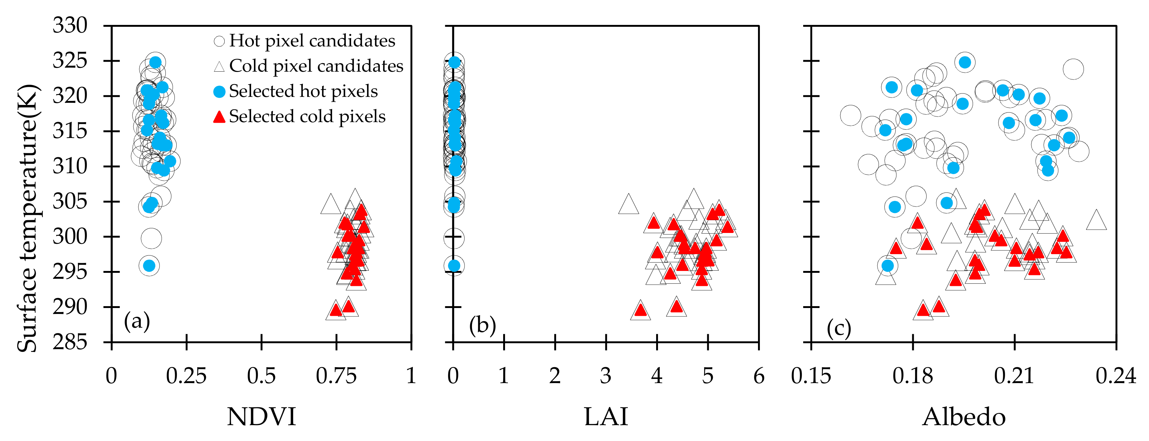
A total of 22 cloud-free and geo-rectified Landsat 7-Enhanced Thematic Mapper Plus (ETM⁺) and Landsat 8-Operational Land Imager (OLI) and Thermal Infrared Sensors (TIRS) images (Path: 37 and Row: 29) were obtained from the US Geological Survey (USGS) (https://earthexplorer.usgs.gov/) for 2017, 2018, and 2019 growing seasons (Table 1). Landsat satellite imagery was preferred over other contemporary satellites because it collects thermal data and has a temporal and spatial resolution of 16 days and 30 m by 30 m, respectively making it easier to map individual agricultural fields. The scan line correction for Landsat 7 was carried out on final instantaneous images using the natural neighborhood interpolation tool of ArcGIS 10.6.1. This tool finds the closest subsets of missing pixels from the pixels surrounding the query point to interpolate a value. It is important to note that the pixels corresponding to the BREBS station location did not have any scan line error. The land use map/cropland data layer (CDL) of the study area for 2017, 2018, and 2019 were obtained from the USDA National Agriculture Statistical Service (NASS). The CDL is a georeferenced raster layer created using moderate resolution satellite imagery and extensive agricultural ground truth. METRIC optionally uses a land-use map to improve the parameterization and estimation of the roughness length for momentum transfer [19,20]. Roughness length for momentum transfer is the height above the plant canopy at which windspeed extrapolates to zero because of form drag of air as well as skin layer friction in between air molecules and surface terrain. The CDL layers were also used to extract water use information of different vegetative surfaces for different irrigation districts in the study regions. Irrigation district boundaries shapefiles were collected from the Wyoming Water Resources Data System (WRDS) and State Climate Office (SCO). The digital elevation model (DEM) provides data on the relief of the earth’s surface in the form of points of elevation. METRIC requires DEM in mountainous terrain where parameters like temperature, pressure, and solar elevation angle vary by slope and aspect. These data were acquired from USDA geospatial data gateway with spatial resolution same as that of Landsat image.

ERDAS imagine (Leica Geosystems Geospatial Imaging, LLC, Englewood, CO, USA) graphical model maker tool was used for geospatial processing of Landsat images. Firstly, the digital numbers (DN) of the images were converted to top of atmosphere radiance and reflectance values using the procedure outline in Landsat 7 and 8 data users’ handbook. Normalized difference vegetation index (NDVI) and soil adjusted vegetation index (SAVI) were computed using reflectance from red and near-infrared bands [45,46]. Leaf area index (LAI) was computed using the empirical equation provided by Bastiaanssen [15], which utilizes SAVI value. Likewise, the solar incidence angle was computed for each pixel of the image using Duffie and Beckman [47] model that considers slope and aspect for each pixel. The slope and aspect of each pixel were computed using DEM. Surface albedo was calculated by integrating the at-surface band reflectance using weighting coefficients [48,49,50]. Surface temperature (Ts) was computed using a modified Planck equation with atmospheric and surface emissivity correction [20]. A neutral-stability-condition atmosphere lapse rate at 6.5 K km⁻¹ in flat terrain and 10 K km⁻¹ in mountainous terrain was considered while calculating DEM corrected Surface temperature (T_s-dem). Likewise, lapse rate change of 2000 m was considered keeping in mind the elevation data of the study area. Moreover, momentum roughness (Z_om), wind speed, and atmospheric pressure were adjusted as mentioned by Allen et al. [20] for use in the mountain model of METRIC.

2.3. METRIC Model

METRIC utilizes multispectral raster images to estimate the energy balance at each pixel of an image and is primarily based upon the principle of energy conservation, i.e., energy arriving at the surface must equal the energy leaving the surface for the same period.

$${\mathrm{R}}_{\mathrm{n}}=\mathrm{LE}+\mathrm{G}+\mathrm{H}$$

(2)

where net radiation (R_n) is the total energy available at the earth surface, soil heat flux (G) is the rate of conductive heat exchange between soil and vegetation, sensible heat flux (H) is the rate of convective and conductive heat exchange between plant canopy and the surrounding air due to temperature difference, and Latent heat (LE) is the instantaneous residual energy available for evapotranspiration which is computed by subtracting G and H from R_n. Figure 3 shows the flowchart of energy balance components and other intermediate parameters estimation by METRIC.

2.3.1. Net Radiation (R_n)

R_n is calculated by subtracting incoming and outgoing radiant fluxes at the top-of-the-atmosphere as:

$${\mathrm{R}}_{\mathrm{n}} = {\mathrm{R}}_{\mathrm{s}}\downarrow - \mathsf{\alpha }{\mathrm{R}}_{\mathrm{s}}\downarrow + {\mathrm{R}}_{\mathrm{L}}\downarrow - {\mathrm{R}}_{\mathrm{L}}\uparrow - \left(1 - {\mathsf{\epsilon }}_{\mathrm{o}}\right) {\mathrm{R}}_{\mathrm{L}}\downarrow$$

(3)

where R_s↓ is the incoming shortwave radiation (W m⁻²), R_L↓ is the incoming longwave radiation (W m⁻²), R_L↑ is the emitted outgoing longwave radiation (W m⁻²),$\mathsf{\alpha }$ is surface albedo (dimensionless) and ε_o is the surface thermal emissivity (dimensionless). The term ((1 − ε_o) R_L↓) in Equation (3) represents a fraction of incoming longwave radiation that is reflected from the earth’s surface. These intermediate parameters of long and short-wave radiation are computed as per Allen et al. [20] and are a function of satellite images, albedo, atmospheric transmissivity, DEM, ground-based weather data, and satellite estimated surface temperature. Surface emissivity (ε_o) was computed using LAI in an empirical equation formulated by Tasumi [51].

2.3.2. Soil Heat Flux (G)

G was empirically calculated as a G/R_n fraction using vegetation indices and surface temperature [51].

$$\frac{\mathrm{G}}{{\mathrm{R}}_{\mathrm{n}}} = 0.05 + 0.18 \times {\mathrm{e}}^{-0.521\mathrm{LAI}} \left(\mathrm{LAI} \ge 0.5\right)$$

(4)

$$\frac{\mathrm{G}}{{\mathrm{R}}_{\mathrm{n}}} = \frac{1.80 \times \left( {\mathrm{T}}_{\mathrm{s}} – 273.15\right)}{{\mathrm{R}}_{\mathrm{n}}}+0.084 (\mathrm{LAI} < 0.5)$$

(5)

where T_s is the surface temperature in Kelvin and LAI (dimensionless) is the leaf area index.

2.3.3. Sensible Heat Flux (H)

H is a function of aerodynamic observations such as u₂, vegetation type and roughness, and surface to air temperature differences ${(\mathrm{T}}_{\mathrm{s}}-{\mathrm{T}}_{\mathrm{a}})$. H is determined using an one-dimensional aerodynamic function within METRIC [15,20] as:

$$\mathrm{H} = \frac{{\mathsf{\rho } \times \mathrm{C}}_{\mathrm{p}} \times \mathrm{dT}}{{\mathrm{r}}_{\mathrm{ah}}}= \frac{{\mathsf{\rho } \times \mathrm{C}}_{\mathrm{p}}{ \times (\mathrm{T}}_{\mathrm{s}} -{ \mathrm{T}}_{\mathrm{a}})}{{\mathrm{r}}_{\mathrm{ah}}}$$

(6)

where $\mathsf{\rho }$ is the air density (kg m⁻³), C_p is the specific heat of the air (1004 J kg⁻¹ K⁻¹), dT is the near-surface air temperature difference ${(\mathrm{T}}_{\mathrm{s}}-{\mathrm{T}}_{\mathrm{a}})$ between two reference heights Z₁ and Z₂, ${\mathrm{T}}_{\mathrm{s}}$ is the surface temperature (K), ${\mathrm{T}}_{\mathrm{a}}$ is the air temperature (K), and r_ah is the aerodynamic resistance to heat transfer (s m⁻¹) over the vertical distance. METRIC utilizes the internal calibration procedure at extreme conditions following surface energy balance algorithms for land (SEBAL) to estimate the dT function. The radiometric temperature available in Landsat thermal band is generally different from the aerodynamic temperature of the surface because of the difference in thermal sensor view angle, land use type and cover fraction, and the surface roughness length of heat and momentum [19]. Therefore, to compensate for uncertainties in the estimation of Ts from satellite, dT function is established for two extreme conditions present in the image viz: cold and hot anchor pixels and is estimated assuming a linear relationship between dT and T_s-dem [15,19,20,24].

dT = b + aT_s-dem

(7)

where T_s-dem is DEM adjusted surface temperature (T_s), a is the slope, and b is the intercept of the plot between dT and T_s-dem for a given satellite image.

Generally, a cold pixel is a well-irrigated field with full crop cover transpiring at potential evapotranspiration rate and a dry pixel is a dry field with approximately zero ETc. Hot and cold pixels are the evaporative extremes of the Landsat scene being analyzed and selection of these extreme pixels is extremely important in the METRIC processing. Therefore, to select the appropriate hot and cold anchor pixels, the maps of NDVI, surface albedo, LAI, Ts, land use, and maps of the image in true and false colors were taken into consideration.

Figure 4 provides a general overview of the hot and cold pixel selection procedure in the study. Cold pixel candidates were selected from the well-irrigated densely vegetated area with NDVI between 0.76 and 0.84, mid season LAI greater than 3 or 4 m² m⁻², surface albedo between 0.18 to 0.24, and a lower surface temperature. Similarly, the hot pixel candidates were selected from the bare agricultural field with NDVI less than 0.20, surface albedo between 0.17 to 0.23, and relatively higher surface temperature. Final selection of the anchor hot and cold pixel for each image was made using the candidate pixels already selected. Tasumi [51] and Tasumi et al. [52] estimated cold pixels to have ET_c rates of about 1.05 times the reference evapotranspiration of alfalfa crop (ETr) except during early and late growing season. To account for any residual evaporation and wetting events before image acquisition, METRIC approximates LE at the hot pixel to be 0.1 [20]. A bare soil evaporation model on a daily time step was used to adjust LE_hot-pixel h.igher than 0.1 in situations with residual soil evaporation from antecedent rainfall. Moreover, the cold and hot pixels were selected within a 20–25 km radius of the meteorological station to counter heterogeneity in weather variables over the Landsat image.

Sensible heat is estimated for both the selected hot and cold pixel using the energy balance equation in respective pixels.

$${\mathrm{H}}_{\mathrm{hot}}={\left({\mathrm{R}}_{\mathrm{n}}-\mathrm{G}\right)}_{\mathrm{hot}}-{\mathrm{LE}}_{\mathrm{hot}}$$

(8)

$${\mathrm{H}}_{\mathrm{cold}}={\left({\mathrm{R}}_{\mathrm{n}}-\mathrm{G}\right)}_{\mathrm{cold}}-1.05\times \mathsf{\lambda }\times {\mathrm{ET}}_{\mathrm{r}}$$

(9)

where λ in H_cold computation refers to latent heat of vaporization (JKg⁻¹). The temperature gradient (dT) is computed for both cold and hot pixels before the final H is calculated.

$$\mathrm{At} \mathrm{cold} \mathrm{pixel}, {\mathrm{dT}}_{\mathrm{cold}} = \frac{{\mathrm{H}}_{\mathrm{cold}} \times { \mathrm{r}}_{\mathrm{ah}-\mathrm{cold}}}{{{\mathsf{\rho }}_{\mathrm{cold}} \times \mathrm{C}}_{\mathrm{p}}}$$

(10)

$$\mathrm{At} \mathrm{hot} \mathrm{pixel}, {\mathrm{dT}}_{\mathrm{hot}} = \frac{{\mathrm{H}}_{\mathrm{hot}} \times { \mathrm{r}}_{\mathrm{ah}-\mathrm{hot}}}{{\mathsf{\rho }}_{\mathrm{hot}}{ \times \mathrm{C}}_{\mathrm{p}}}$$

(11)

The aerodynamic resistance to the transfer of the heat from the evaporating surface to the air above the canopy is calculated as given by Bastiaanssen et al. [15].

$${\mathrm{r}}_{\mathrm{ah}} = \frac{1}{{\mathrm{k} \times \mathrm{u}}_{*}} \ln \left(\frac{{\mathrm{Z}}_2}{{\mathrm{Z}}_1}\right)$$

(12)

where z₁ and z₂ are lower and upper reference heights (m) above zero plane displacement (d) of the vegetation and are assigned to be 0.1 m and 2 m respectively [15]. ${\mathrm{u}}_{*}$ is the friction velocity (m s⁻¹) computed during the first iteration of H and k is the Von Karman’s constant (0.41). The ${\mathrm{u}}_{*}$ at the first iteration, is defined by the relation:

$${\mathrm{u}}_{*} = \frac{\mathrm{K} \times { \mathrm{U}}_{200}}{\ln \left(\frac{200}{{\mathrm{Z}}_{\mathrm{om}}}\right)}$$

(13)

where U₂₀₀ is the wind speed at the blending height (200 m) above the weather station, z_om (m) is the momentum roughness length calculated using a land-use map for each image pixel. z_om is calculated as a function of LAI [51].

z_om = 0.018 × LAI

(14)

The sensible heat flux (H) is then calculated for each pixel using Equation (6). However, this event is the first estimation of H and is calculated assuming neutral atmospheric conditions. To counter unstable atmospheric conditions, H is computed through the number of iterations until r_ah is stabilized. At each iteration, values for dT_cold, dT_hot, air temperature, air density, r_ah, U_*, and H is corrected and is continued until successive values for dT_hot and r_ah at the hot pixel have stabilized. Usually, stability is achieved after 4–5 iterations. The Monin–Obukhov length (L) is used to stabilize the atmosphere (boundary layer) where turbulence is generated by the buoyancy effect of surface heating. The value of L is zero for neutral, positive for stable, and negative for unstable atmospheric conditions.

$$\mathrm{L} = \frac{{\mathsf{\rho } \times \mathrm{C}}_{\mathrm{p}}\times { \mathrm{u}}_{*}{}^3\times { \mathrm{T}}_{\mathrm{s}}}{\mathrm{K}\times \mathrm{g}\times \mathrm{H}}$$

(15)

where g is the gravitational constant (9.8 ms⁻²).

2.3.4. Estimation of Instantaneous, Daily, Monthly and Seasonal Crop Evapotranspiration (ET_c)

Instantaneous ET (ET_inst) at the time of Landsat overpass is computed as residual of the surface energy balance by subtracting instantaneous G and H are from R_n as:

$${\mathrm{ET}}_{\mathrm{inst}} = \frac{3600 \times \left({\mathrm{R}}_{\mathrm{n}}-\mathrm{G}-\mathrm{H}\right)}{{\lambda \times \mathsf{\rho }}_{\mathrm{w}}}$$

(16)

where ${\mathsf{\rho }}_{\mathrm{w}}$ is the density of water (~1000 kgm⁻³). METRIC utilizes reference ET fraction (ET_rF) value to compute daily and periodic ET_c [20]. ET_rF (dimensionless) is calculated for each pixel as a ratio of ET_inst to the reference ET values at the time of image acquisition.

$${\mathrm{ET}}_{\mathrm{r}}\mathrm{F} = \frac{{\mathrm{ET}}_{\mathrm{inst}}}{{\mathrm{ET}}_{\mathrm{r}}}$$

(17)

where ETr is the alfalfa reference evapotranspiration calculated using the standardized ASCE Penman–Monteith equation [53] on an hourly basis. It is assumed that ET_rF (equivalent to crop coefficient) values remain constant throughout the day and the use of it minimizes the impact of advective heat on ETc [54]. The daily evapotranspiration (ET₂₄) rate (mm d⁻¹) for each image pixel is then computed as:

ET₂₄ = ET_rF × ET_r-24

(18)

where ET_r-24 is 24-h ET_r and is calculated by summing hourly ET_r values over the day of image. To estimate periodic ET_c values, both linear and cubic spline methods of interpolation were employed. Linear interpolation [55] was done by interpolating ET_rF between successive image dates. The interpolated values were then multiplied by ET_r-24 to obtain ET_24, which is then summed up on monthly and seasonal baisis. On the other hand, cubic spline [19] is reported to get a smooth and curvilinear bend as of the typical crop coefficient curve of annual crops [56]. Rather than taking all the data points at once to fit one polynomial, spline interpolation fits a polynomial function between two adjacent data points. For example, 4 images (data points) will have three polynomials fitted in between. A third-degree polynomial (cubic polynomial) is used to get a smooth fit between each spline. Thus, cubic spline interpolation requires two images on either side of the month and at least one ET_rF image per month in a growing season. As such, it requires at least 5 images to interpolate for a month. Likewise, synthetic points (ET_rF_synthetic) were computed for the beginning and end of the growing season (ET_c is dominated by evaporation) to be able to start and end the interpolation. Daily actual evaporation (E_a), estimated using the soil water balance method [10], and ET_r were used to calculate the synthetic points.

$${\mathrm{ET}}_{\mathrm{r}}{\mathrm{F}}_{\mathrm{synthetic}} = {{\displaystyle \sum }}_{1\mathrm{st} \mathrm{day} \mathrm{of} \mathrm{summation}}^{\mathrm{last} \mathrm{day} \mathrm{of} \mathrm{summation}}\left(\frac{{\mathrm{E}}_{\mathrm{a}}}{{\mathrm{ET}}_{\mathrm{r}}}\right)$$

(19)

$${\mathrm{ET}}_{\mathrm{month}} = {{\displaystyle \sum }}_{1\mathrm{st} \mathrm{day} \mathrm{of} \mathrm{month}}^{\mathrm{last} \mathrm{day} \mathrm{of} \mathrm{month}}\left(\left({\mathrm{ET}}_{\mathrm{r}}{\mathrm{F}}_{\mathrm{i}}\right)\times \left({\mathrm{ET}}_{\mathrm{r}}{24}_{\mathrm{i}}\right)\right)$$

(20)

where ET_month (mm) is the monthly cumulative ET_c from day 1st to last day of the month, ET_rF_i is the interpolated ET_rF for a month and ET_r24i is the 24-h ET_r for a month. Seasonal estimates of ET_c were then obtained by summing up the monthly ET_c values. The METRIC estimated instantaneous and periodic fluxes were compared with BREBS measured fluxes. Root mean square error (RMSE) and Nash–Sutcliffe’s efficiency (NSE) were used as the main criterion to judge the accuracy and reliability of the METRIC model for estimating ET_c and other surface energy fluxes.

$$\mathrm{RMSE}= \sqrt{\frac{{{\displaystyle \sum }}_{\mathrm{i}=1}^{\mathrm{n}}{\left(\mathrm{O}-\mathrm{P}\right)}^2}{\mathrm{n}}}$$

(21)

$$\mathrm{NSE}=1-\left( \frac{{{\displaystyle \sum }}_{\mathrm{i}=1}^{\mathrm{n}}{\left(\mathrm{O}-\mathrm{P}\right)}^2}{{{\displaystyle \sum }}_{\mathrm{i}=1}^{\mathrm{n}}{\left(\mathrm{O}-{\mathrm{O}}_{\mathrm{mean}}\right)}^2}\right)$$

(22)

where O and P is the observed and METRIC predicted surface energy balance fluxes, O_mean is the mean of observed energy balance fluxes, and n is the number of observations.

3. Result and Discussions

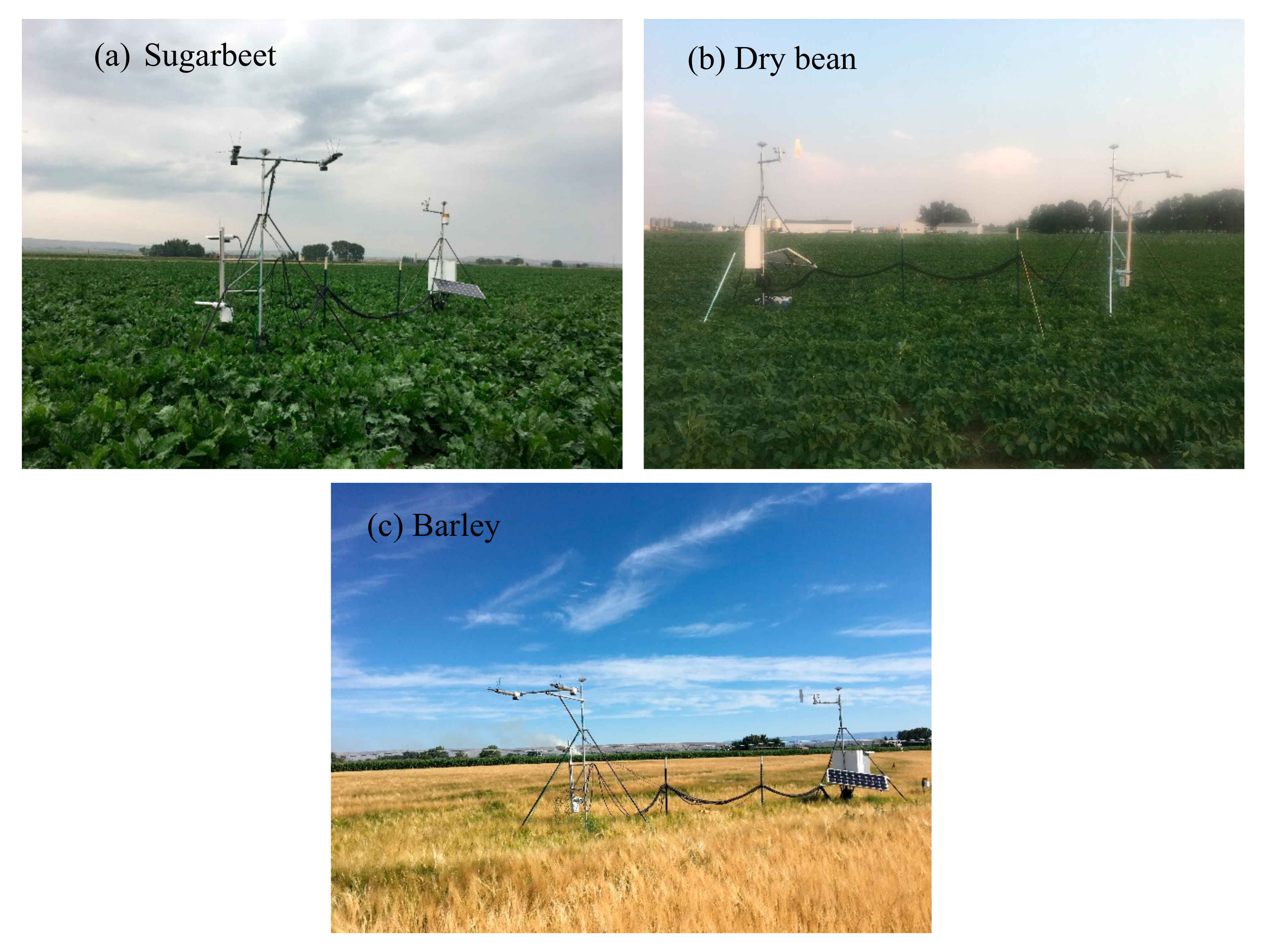
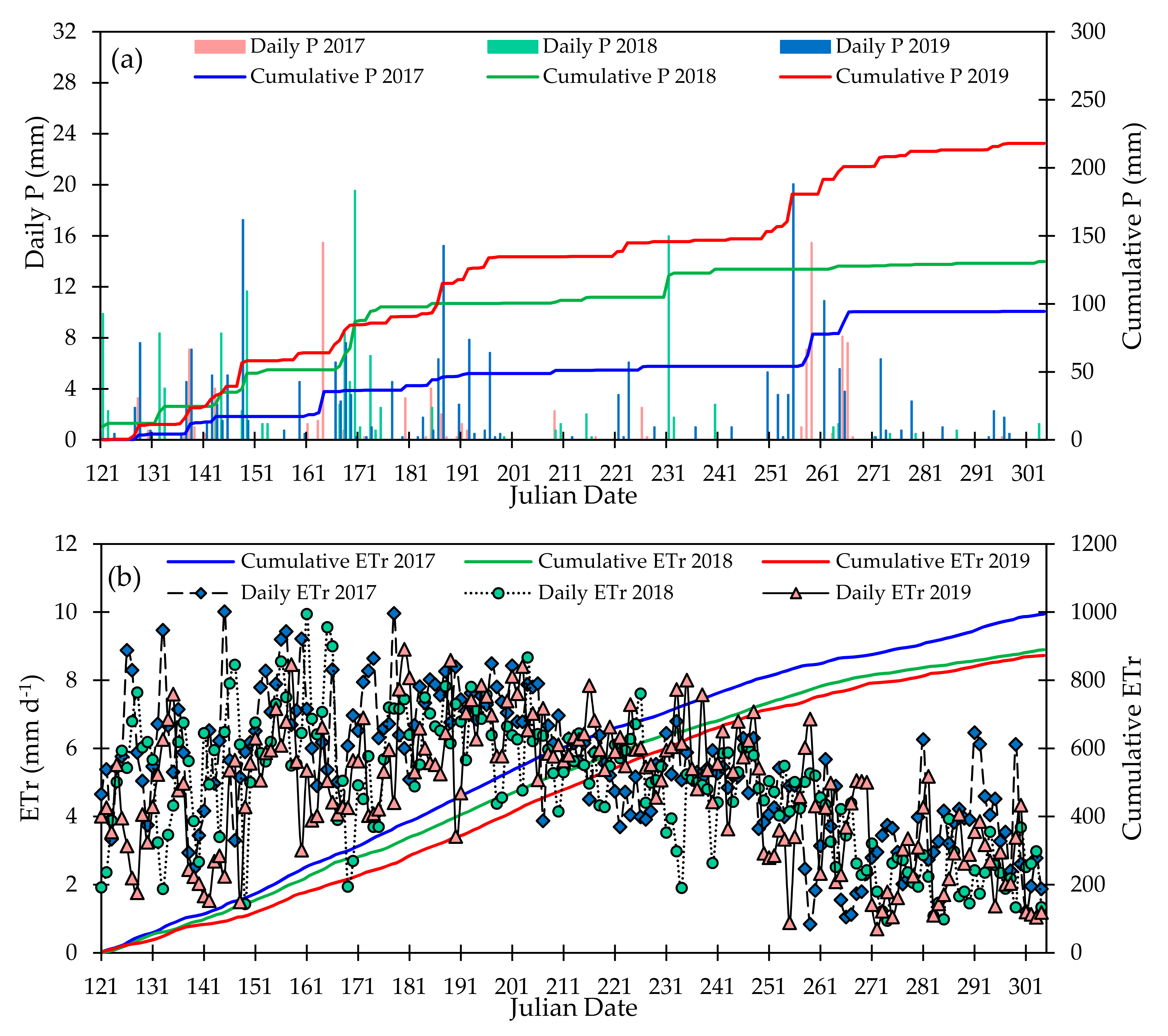
3.1. Weather Conditions

Figure 5 represents daily and cumulative P and ET_r during 2017, 2018, and 2019 growing seasons (May to September). Substantial variations were observed in weather variables during each of the three years. Compared to long-term average values, 2017 had below normal precipitation and higher ETr. A total of 32 and 30 precipitation events occurred in 2017 and 2018, respectively, compared to 56 events in 2019. The total seasonal P of 94 mm, 128 mm, and 20817 mm was observed in 2017, 2018, and 2019, respectively. Likewise, September 2017 (40 mm), June 2018 (48 mm), and May 2019 (58 mm) were the months receiving highest cumulative precipitation in their respective years. Greater evaporative demand existed in 2017 and 2018 compared to 2019. The ETr ranged from 0.84 to 10.01 mmd⁻¹, 1.23 to 9.94 mmd⁻¹, and 0.70 to 8.9 mmd⁻¹, with an average of 5.7 mmd⁻¹, 5.4 mmd⁻¹, and 5.2 mmd⁻¹ for 2017, 2018, and 2019, respectively. Cumulative ETr was highest in 2017 (883 mm) followed by 2018 (820 mm), and 2019 (794 mm) growing season. The month of July observed highest ET_r (224 mm in 2017, 196 mm in 2018, and 198 mm in 2019) in each of the growing season. Likewise, the month of May witnessed some days with relatively higher ET_r (Figure 5b).

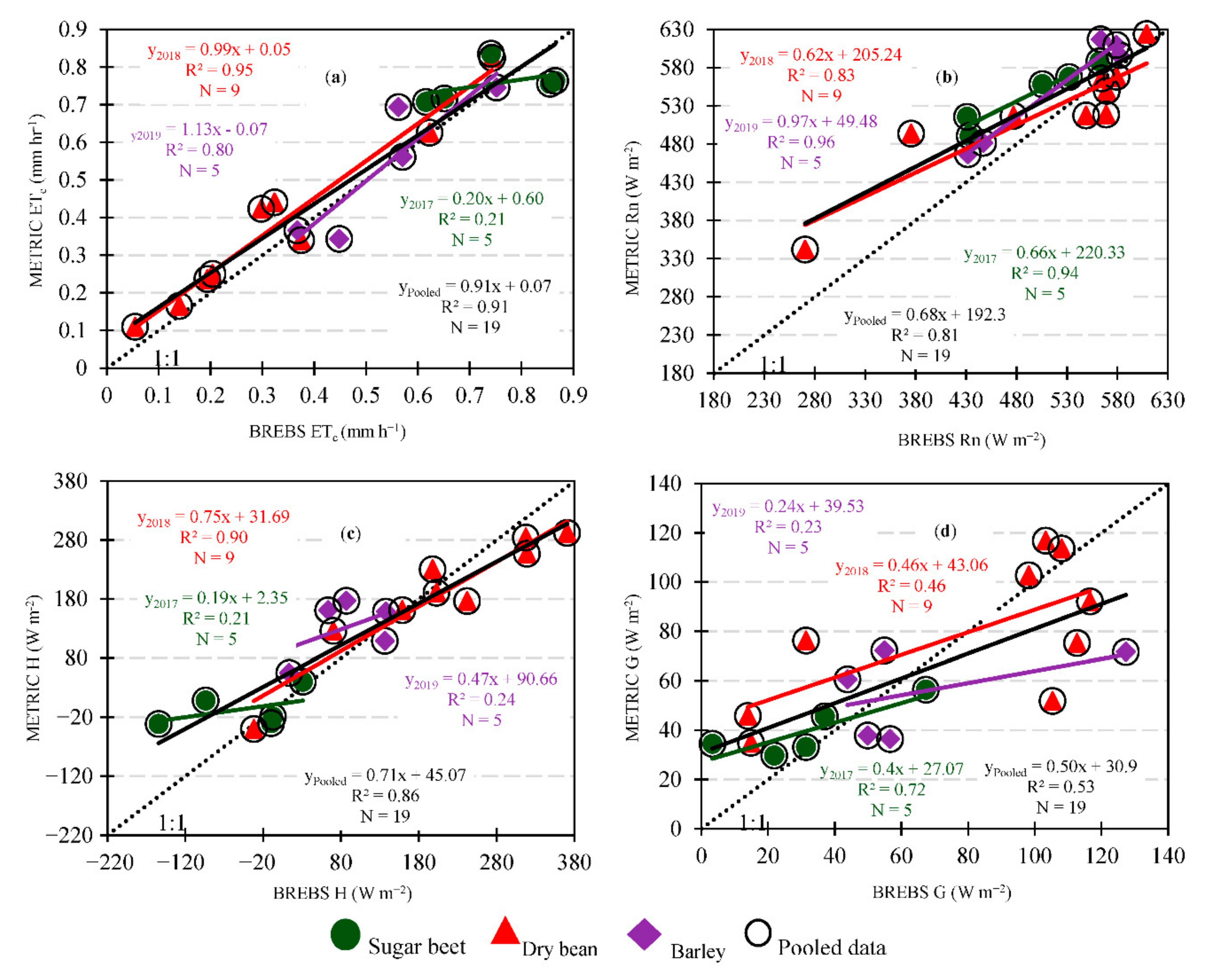
3.2. Comparison of METRIC Estimated and Measured Surface Energy Balance Fluxes

Several uncertainties may be associated with the satellite retrievals of energy balance systems including sensor pixel scale, sensor accuracy, etc. Thus, a comparison of satellite retrievals with ground-based measurements becomes inevitable to garner confidence on the final output being accurately estimated. Figure 6 reflects the evaluation of estimated vs. measured instantaneous surface energy balance fluxes at the BREBS flux tower footprint in Powell Research and Extension Center, Powell, WY. The BREBS values were retrieved at satellite overpass time (11:00 A.M. MST) to compare with corresponding METRIC determined energy balance components. A total of five different data points from the 2017 growing season (July–September), nine different data points from the 2018 growing season (May–October), and five different data points from the 2019 growing season (June–September) along with the pooled data from all the growing seasons were used in the analyses. Similarly,

Table 2. Statistical comparison between METRIC estimated and BREBS measured crop evapotranspiration (ET_c, mm h⁻¹), net radiation (R_n, Wm⁻²), soil heat (G, Wm⁻²), and sensible heat (H, Wm⁻²) for 2017, 2018, 2019, and pooled data from all the growing seasons (N = number of data points, R² = coefficient of determination, SD = standard deviation, S = slope, RMSE = root mean square error, NSE = Nash-Sutcliffe’s efficiency).

Flux	Year	Surface	N	R2	Avg. BREBS	Avg. METRIC	SD BREBS	SD METRIC	S	RMSE	NSE
ETc	2017	Sugarbeet	5	0.21	0.75	0.76	0.11	0.05	0.20	0.09	0.20
	2018	Dry Bean	9	0.95 *	0.33	0.38	0.23	0.23	0.99 *	0.07	0.89
	2019	Barley	5	0.80 *	0.54	0.54	0.15	0.18	1.1 *	0.08	0.67
	Pooled		19	0.91 *	0.49	0.52	0.25	0.24	0.91 *	0.08	0.90
Rn	2017	Sugarbeet	5	0.94 *	492.8	544.3	58.8	40	0.66 *	55.3	0.95
	2018	Dry Bean	9	0.83 *	506.9	522	113.2	77.9	0.62 *	52.7	0.76
	2019	Barley	5	0.96 *	520.5	554.5	74.7	73.8	0.97 *	36.2	0.70
	Pooled		19	0.81 *	506.8	536.4	88.4	66.9	0.68 *	49.6	0.67
G	2017	Sugarbeet	5	0.72	32.2	39.9	23.4	11	0.4	15.7	0.44
	2018	Dry Bean	9	0.46 *	78.3	78.8	44.2	29.9	0.46 *	30.8	0.46
	2019	Barley	5	0.23	66.5	55.8	34.3	17.6	0.24	29.1	0.1
	Pooled		19	0.53 *	63.04	62.5	40.5	28	0.50	27.1	0.53
H	2017	Sugarbeet	5	0.21	−46.9	−6.4	75.4	30.5	0.19	72.5	−0.15
	2018	Dry Bean	9	0.90 *	205.1	186.4	127.9	102	0.75	46.8	0.85
	2019	Barley	5	0.24	87.6	132	52.3	50	0.47	64	−0.87
	Pooled		19	0.86 *	107.8	121.4	143.7	109.9	0.71 *	59.2	0.82

* The correlation between measured and estimated flux is significant and slope of the regression line was significantly different from zero (p = 0.05).

provides a statistical comparison between METRIC estimated and BREBS measured energy balance components. The R², RMSE, and NSE were used to assess the error associated with each component. The following section discusses the comparison of METRIC estimated instantaneous energy balance fluxes (R_n, G, H, and ET_c) of the pixel corresponding to the geographic location of the BREBS towers.

3.2.1. Instantaneous ET_c (ET_inst)

Figure 6a indicates a good correlation between METRIC estimated and BREBS measured ET_inst with R² values ranging between 0.21 to 0.95 and slopes between 0.2 to 1.13. For pooled data points, the linear regression model explains 91% of all the variance in the estimated ET_inst values. The slope of the regression coefficient of pooled data (0.91) close to unity (p-value < 0.05) indicates a strong fit and low systematic error between modeled and measured ET_inst. The average ET_inst for all data points over three vegetative surfaces was 0.52 mm h⁻¹ (355 W m⁻²) as compared to the BREBS measurement of 0.49 mm h⁻¹ (336 W m⁻²), with pooled RMSE of 0.08 mm h⁻¹ and NSE of 0.90. Table 2 represents a comparison of METRIC estimate ET_inst with BREBS measurement for individual surfaces. Overall, a good correlation was observed between measured and estimated ET_c for all three vegetative surfaces, with R² ranging from 0.21 for sugar beet in 2017 to 0.95 for dry bean in 2018. A relatively lower R² (0.21), slope (0.20) and NSE (0.21) for 2017 ET_inst indicate low performance of the model (Table 2). The regression analysis showed that the correlation is not significant and slope of the regression line was significantly different from unity (p-value > 0.05). The BREBS tower was installed on June 2017 which resulted only handful of images (5) in mid to late growing season for analysis in 2017. This resulted in a skewness of data and errors in one direction causing lower NSE, R², and slope values. On the other hand, 2018 and 2019 had images spread across the growing season. A comparison of the individual vegetation surfaces revealed that the METRIC model overestimated ET_inst by 1.4%, 15.8%, and 0.4% for 2017, 2018, and 2019, respectively, as compared to BREBS measurements (Table 2). Higher overestimation in 2018 is due to the fact that three out of the nine images were analyzed before planting and after harvest when only crop residue was available at the surface. For example, the combined overestimation of 41% was observed for the three images when only crop residue was available at the surface compared to 9.8% when the image was analyzed within the growing season. Variation in crop residue at the surface can alter the surface temperature which may result in more variation in ET_c available at the surface [13,57]. A similar improvement in results was reported by Allen et al. [19]. They compared METRIC estimated ET_c with lysimeter measured ET_c using eight Landsat images acquired from April to September and reported 30% averaged absolute differences for sugar beet crop (R² = 0.82). When they omitted one image date of drying bare soil following P, the average absolute difference was only 14%. The maximum difference in ET_inst of 0.13 mm h⁻¹ was observed in 2019 on 21 July, which could attribute to the continuous P events from 14 July to 17 July which resulted in increased soil surface moisture and decreased surface temperature, thus resulting in higher bias from the measured data [58].

3.2.2. Net Radiation (R_n)

METRIC estimated R_n had an R² value of 0.83 to 0.96 and a slope of 0.62 to 0.97 when compared with corresponding BREBS fluxes (Figure 6b). The average METRIC estimated R_n for the pooled dataset was 507 W m⁻² (SD = 88 W m⁻²) compared to BREBS measured R_n of 537 W m⁻² (SD = 67 W m⁻²). The RMSE value for R_n was found to be ranging from 36.2 to 55.3 W m⁻² and NSE between 0.70 to 0.95 (Table 2). Pooled data points had R² of 0.81, slope of 0.68, RMSE value of 49.6 W m⁻², and NSE of 0.67 (Figure 6b). Table 2 indicates the average R_n to be overestimated by 10.5%, 3%, 6.5%, and 5.8% for 2017, 2018, 2019, and pooled data points, respectively. Similar observations were made by Singh et al. [35], who used METRIC model in conjunction with wet-METRIC (a modified version of METRIC) model for analyzing Landsat images in the three sites of Mid-western United States. They reported model-estimated net radiation (R_n) to be within −12%, −11.4%, and −6.3% of the eddy covariance measurement for three different study sites with R² of 0.95. R_n is a very complex variable and varies with the complexity of the underlying surface heterogeneity. For example, a heterogeneous surface influences the surface radiation properties, e.g., surface albedo and emissivity, and thereby impacts the fraction of photosynthetically active radiation absorbed crop transpiration rate and surface energy budgets. For example, as observed from Figure 6b, the maximum variation in R_n was observed on 12 September and 22 October 2018, when only crop residue was available at the surface. Horton et al. [57] reported that crop residue that alters surface evaporation and soil moisture content can affect both the shortwave albedo and longwave emissivity, and hence R_n.

3.2.3. Sensible Heat Flux (H)

Figure 6c and Table 2 represent the comparison of METRIC derived H with BREBS measured H along with statistical analysis. Overall good correlation was observed between METRIC estimated H and BREBS measured instantaneous H values with R² between 0.21 to 0.9 while the value for slope was between 0.19 to 0.75 (Figure 6c). When pooled data were taken into consideration, R² value was 0.86 with a slope of 0.71. Lower RMSE value was observed in 2018 (46.8 W m⁻²) as compared to 2017 (72.5 W m⁻²) and 2019 (64 W m⁻²) image dates (Table 2). However, when pooled data points were considered, the average METRIC estimated H was 121 W m⁻² which is 12.6% higher than field measurements (average H = 107 W m⁻²) with RMSE 59.2 W m⁻² and NSE of 0.82 (Table 2). A negative NSE during 2017 (−0.15) and 2019 (−0.87) indicates the model had less predictive skill during those periods. The partitioning of available energy (R_n-G) to LE for each satellite date revealed some image dates where advection is prominent (LE/(R_n-G) > 1) (data not shown). For example, negative values of Hwere observed for both METRIC estimated H and BREBS H, especially in 2017 on 15 July, 31 July, 1 September, and 9 September (Figure 6c). This indicates the movement of energy from the air to the plant canopy and additional energy being used by the crop to meet the high ET demand on that day. This may be due to the already harvested barley field surrounding the BREBS sugar beet field that acted as a source for advective heat. In addition, natural vegetation covers about 83% of our study area surrounding the cropland which also acted as a source of advective heat. However, compared to 2017, in 2018 and 2019, the ratio of LE/(R_n-G) was observed to be less than 1 on most image dates; this may be due to higher P and lower T_air in 2018 and 2019, where the average P was 19 mm and 81 mm higher than 2017 and average T_air was 0.50 °C and 0.74 °C lower than 2017, which reduce the effect of advective heat from surrounding areas. On average, H was better estimated during 2018 image dates where average METRIC estimated H differed from BREBS H by −9.1% as compared to 2017 (−86.4%) and 2019 (50.8%) image dates (Table 2). Poor estimation of H in 2017 and 2019 can be associated with the irrigation and P events that occurred before Landsat overpass time. This created difficulty in choosing a suitable hot pixel candidate having LE approximately zero [35,59]. Similar observations were made by Singh et al. [35] who reported estimated and measured sensible heat had predictive error and R² value of 48.3% (R² = 0.73), 15.2% (R² = 0.71), and −2.4% (R² = 0.03) for three different sites in the Mid-western United States. Kilic et al. [60] reported RMSE of 46.5 W m⁻² and 31.5 W m⁻² in H during the 2005 and 2006 growing seasons in Southeast Nebraska, similar to the RSME in this study in 2017.

3.2.4. Soil Heat Flux (G)

G is one of the key components in the surface energy budget used to estimate the available energy to be partitioned into H and LE. A moderate correlation was observed between METRIC estimated G and BREBS measured G with R² in between 0.23 to 0.72 and slope in between 0.24 to 0.46 (Figure 6d). Pooled G data points had R² of 0.53 and a slope of 0.5 (Figure 6d). METRIC estimated average G differed by 23.9%, 0.75%, −16.1%, and −0.8% for 2017, 2018, 2019, and pooled data, respectively, when compared with BREBS fluxes (Table 2). The RMSE value for the growing seasons ranged between 15.7 to 30.8 W m⁻² while pooled data points had RMSE of 27.1 W m⁻² (Table 2). Likewise, NSE value for the growing seasons considered ranged between 0.1 and 0.46 while pooled data points had NSE of 0.53 (Table 2). In general, G is a relatively small component in energy balance, and its estimation via model is usually difficult because of changes occurring in soil properties such as in conductivity, temperature, and heat capacity with a change in moisture and vegetation of soil. Singh et al. [35], in their study in mid-west USA, reported estimated and measured soil heat flux (G) differing by 16.5%, −6.6%, and −30.3% for three different sites. The same study showed a low R² value of 0.03, 0.36, and 0.33 for soil heat flux. Similar results were found by Irmak et al. [61], who reported a higher RMSD of 48.6 W m⁻² in 2005 on irrigated continuous maize at three sites near Mead, Nebraska. They used a different remote sensing model to predict G at the Mead and Clay Center locations, and the reported difference in G ranged from 36.3 to 62.6 W m⁻² due to differences in soil properties, measurement of G (sensor depth and distance between sensors), and surface conditions at the different locations.

It is important to note that there are many sources of uncertainties associated with the comparison of BREBS measured and modeled fluxes including model algorithm (model assumptions), tower observations (systematic and unsystematic bias), scaling issues (flux footprint), and management practices. For example, BREBS assumes the eddy diffusivities of heat and water vapor to be equal. Studies [62,63] have revealed that these diffusitives may not be equal in some cases resulting a force closure of surface energy budget. Likewise, Barr et al. [62] reported that BREBS favoured prediction of LE as compared to H. The potential effect of condensation in the surface energy balance fluxes is small and has not been considered in this research. Condensation is more pronounced during the night time when RH is at 91–99% and the leaves are cooler than the surrounding air and approaches dew point temperature [64]. Careful analysis of average hourly RH data from BREBS indicated RH barely goes above 90% in the actice growing season where most of the staelite images were collected (data not shown). A similar oberevation was made by Sharma [65] in the semi-arid grass land region of New South Wales, Australia where it was reported that dew fall amounted to 8.7% of ET_c in winter, 4.7% of ET_c in autumn, 1.6% of ET_c in spring season, and as low as 1% of actual or pan evaporation in warmer months.

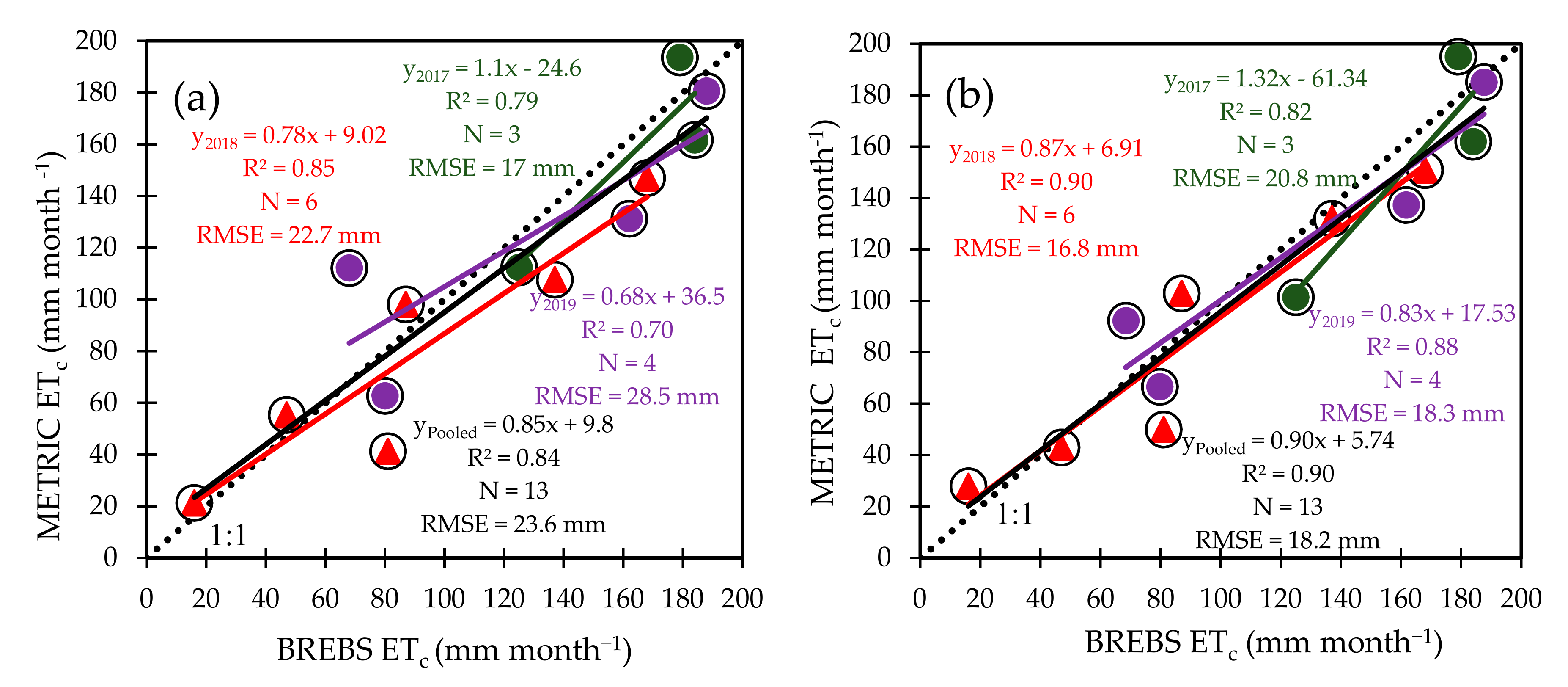
3.3. Comparison of METRIC Estimated and BREBS Measured Monthly ET_c

METRIC estimated monthly ET_c values during 2017 (3 data points), 2018 (6 data points), and 2019 (4 data points) growing seasons were obtained employing linear and cubic spline interpolation method. Cubic spline interpolation observed a better correlation between estimated and measured monthly values with high R² ranging from 0.82 to 0.9, slope between 0.83 to 1.32, and RMSE in between 16.8 to 20.8 mm (Figure 7b). On the other hand, linear interpolation had moderate R² in between 0.7 to 0.85, slope between 0.68 to 1.1, and RMSE in between 17 to 28.5 mm (Figure 7a). Pooled data (13 data points) for cubic spline had R² and slope at 0.9 and RMSE at 18.2 mm, whereas for linear interpolation the values were at 0.84, 0.85 and 23.6 mm for R², slope and RMSE respectively (Figure 7a,b). Cubic spline interpolation underestimated seasonal ET_c by 6%, 5.4%, and 3.2%, while linear interpolation underestimated seasonal ET_c by 4%, 12%, and 2% during 2017, 2018, and 2019 growing seasons (

Table 3. Statistical comparison between METRIC estimated (via linear and cubic spline interpolation) and BREBS derived monthly and seasonal ETc during 2017, 2018, and 2019 growing seasons.

Year	Month	Surface	BREBS ETc	METRIC ETc (C. Spline)	METRIC ETc (Linear)	% Error (C. Spline)	% Error (Linear)
2017	July	Sugarbeet	179	195.1	193.7	9	8.2
2017	August	Sugarbeet	184	162	161.7	−12	−12.1
2017	September	Sugarbeet	125	101.5	112.5	−18.8	−10
2017	(July–September)	Sugarbeet	488	459	468	−6	−4
2018	May	Dry bean	47	43	55.4	−8.5	18
2018	June	Dry bean	81	50	41.3	−38.3	−49
2018	July	Dry bean	137	132	107.7	−3.6	−21.4
2018	August	Dry bean	168	151	147	−10.1	−12.5
2018	September	Dry bean	87	103	98.1	18.4	12.8
2018	October	Dry bean	16	28	21.4	75	33.4
2018	(May–October)	Dry bean	536	507	471	−5.4	−12
2019	June	Barley	161.7	137.4	131.3	−15.1	−19
2019	July	Barley	187.6	185.1	180.7	−1.3	−3.9
2019	August	Barley	68.4	92.3	112.2	34.9	65
2019	September	Barley	79.7	66.7	62.8	−16.4	−21
2019	(June–September)	Barley	497.5	481.5	487	−3.2	−2

). The biggest discrepancy between measured and estimated monthly ET_c values was observed during times when the BREBS flux tower footprint was devoid of any crops or the crops at footprint were not actively transpiring (Table 3). During the 2018 growing season, METRIC estimation of monthly ET_c values ranged between −49% (underestimation) in June (dry bean at BREBS footprint planted on 5 June) to 75% (overestimation) in October (dry bean at BREBS footprint harvested on 10 September) (Table 3). Allen et al. [19], in a study regarding sugar beet, observed estimated periodic ET_c differing by −28% on 7 July to 107% on 4 May as compared to lysimeter measured ET_c. However, this difference in data decreased to less than 1% when cumulative ET_c values for the growing season were compared. Similarly, Allen et al. [19], considering an irrigated meadow, observed METRIC estimated monthly ET_c to be ±16% of the lysimeter measurement. However, in the same study, the difference was reduced to 4% when METRIC estimated and lysimeter measured growing season ET_c (July to October) was considered. This decrease in the difference between estimated and measured growing season ET_c values can be linked with the error associated being randomly distributed (monthly ET_c values being both over and underestimated) tending to cancel while computing a cumulative growing season value [19]. However, both interpolation methods performed well, with cubic interpolation performing slightly better than linear interpolation, owing to its lower and consistent RMSE and % error. Therefore, in this study, cubic interpolation estimated ETc values were used to quantify and map the seasonal ETc and for other analysis. Further quantification and mapping of periodic ET_c in this study was done using cubic spline interpolated images.

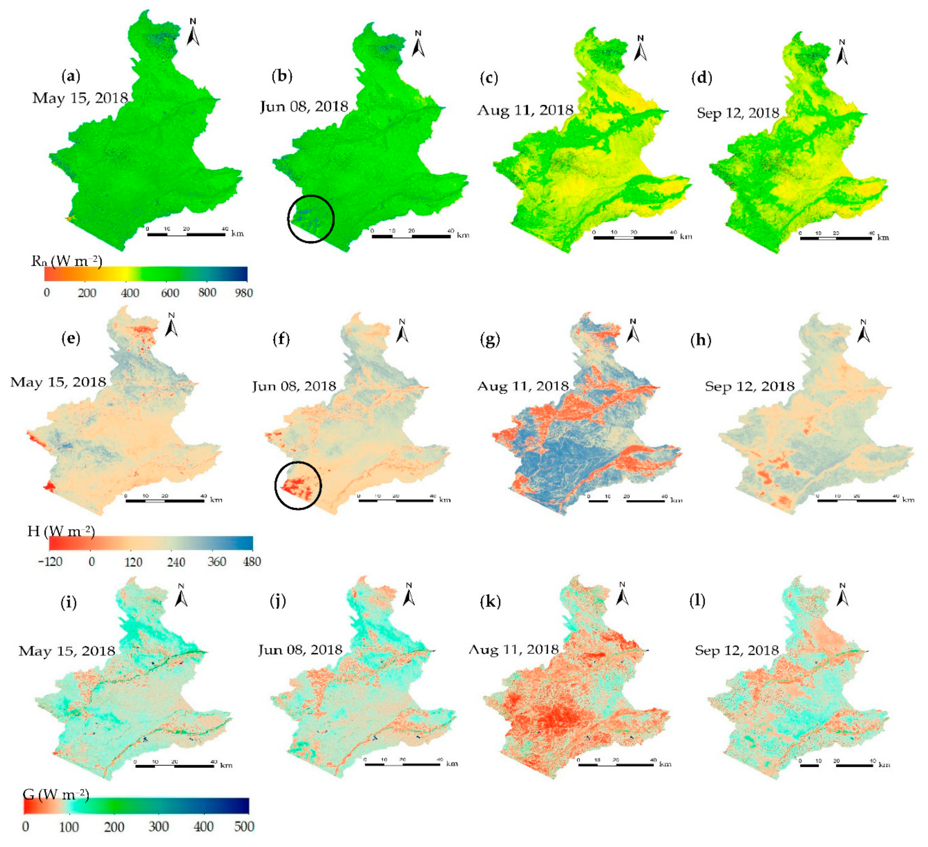
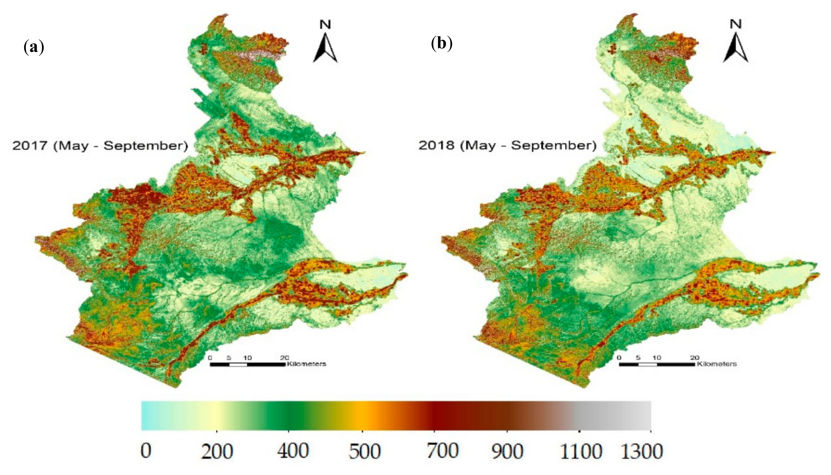
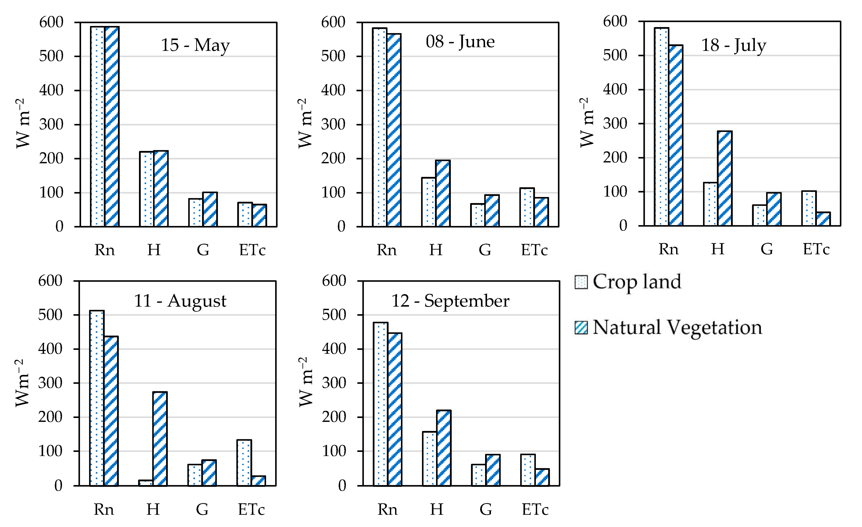
3.4. Mapping Spatio-Temporal Variation of Surface Energy Balance Components

Satellite images, unlike traditional and conventional methods of measurement, provide an excellent means to determine and map the spatial and temporal variation of surface energy balance fluxes and vegetative indices. The spatial (space) and temporal (time) variability on a regional scale is a function of topography, weather parameters, climate, soil characteristics, land-use type, and management practices.

3.4.1. Spatio-Temporal Variation of Net Radiation (Rn), Sensible Heat (H), and Soil Heat (G) Flux

Figure 8 depicts the early, mid, and late-season Spatio-temporal variability of Rn, H, and G for 2018 crop growing season. In general, the intensity of R_s and thus the R_n increases gradually after the March equinox and starts decreasing when the September equinox is reached [66]. A similar pattern is observed in our case where a higher R_n value is observed from May to August. Clouded parts in the images over estimates Rn value as evidenced in the 8 June image where the Rn climbed up to 980 W m⁻². As more and more energy gets partitioned into ET_c, the H value decreases (occasionally negative) as the growing season moves forward. Negative sensible heat estimation occurred occasionally when the temperature and vapor pressure of surrounding air were higher as compared to plant surface temperature and air vapor pressure surrounding the plant, resulting in a flow of heat from surrounding air to the plant. Clouded parts in the image can cause a drastic reduction in the value of H, obvious in 8 June image in Figure 8f, where the H value hovered around −125 W m⁻². Similarly, lower soil heat value was estimated for cropland during mid-season because of higher LAI and NDVI during this time. High ground cover decreases the conduction of R_n to the soil surface. The opposite happens during the early season when crops have less effective ground cover. Similarly, a lower soil heat value at the end of the growing season indicated less availability of net radiant energy. The overestimation of G value can be apparent in clouded parts of the images. A higher G value reaching up to 500 W m⁻² is from the open water area of the image. Unlike land surface, G is a larger and more important component for water bodies [67].

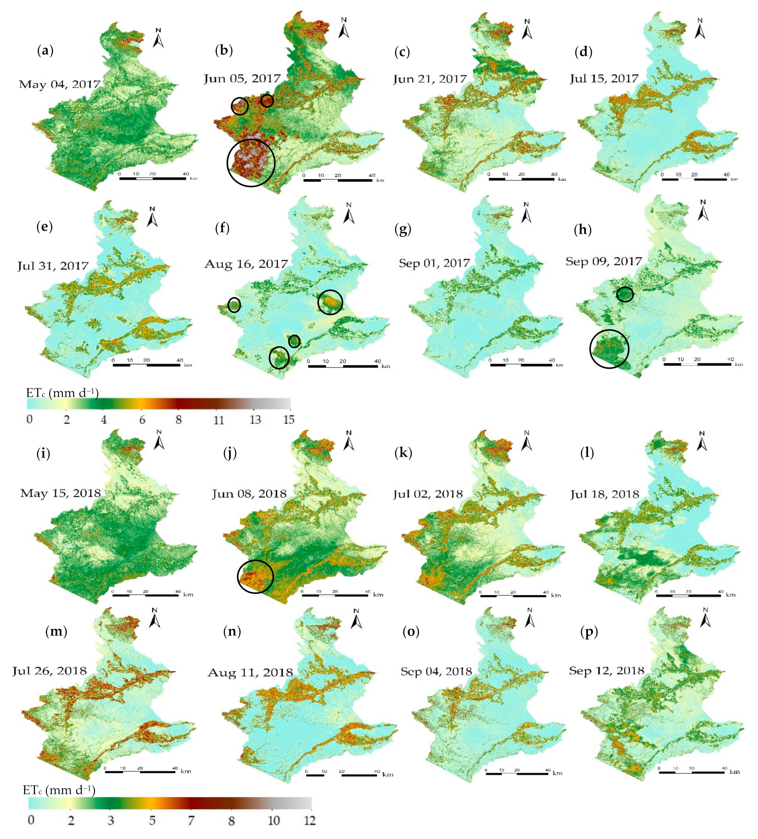
3.4.2. Spatio-Temporal Variation of Evapotranspiration (ET_c)

In METRIC, ET_c is estimated as a residual of the surface energy balance fluxes and occurs through energy exchange at vegetation surface via H or R_n. In general, ET_c is a function of weather parameters, crop characteristics, soil properties, and crop cultivation and management practices. Figure 9 shows the spatial distribution of daily ET_c for Landsat overpasses at scattered times in the 2017 and 2018 growing seasons. Over the production crop areas, the ET_c rate was low during the beginning of the crop season and increased as the season moved forward. During the late season, as plants approached physiological maturity, the ET_c rate declined. On the contrary, higher ET_c was observed over the natural vegetation early in the season (May and June) and strats decrasing as the season progressed. During the early season, evaporation dominates the ET_c while as the season progresses, transpiration forms the major part of ET_c. Most of the variability in ET_c was due to the diverse cropping systems and agronomic practices across the study area. Clouded parts of the image, depending upon the cloud thickness, will experience an overestimated ET values, reaching up to 14.8 mm (5 June 2017) in this study.

3.5. Mapping Spatio-Temporal Variation of Cumulative Seasonal Evapotranspiration

Figure 10 reflects the spatio-temporal variation of cumulative seasonal ET_c during the 2017 and 2018 (May–September) growing season periods. The METRIC estimated average growing season ET_c for cropland was 644 mm and 575 mm for 2017 and 2018, respectively. Similarly, the METRIC estimated average growing season ET_c for natural vegetation was 311 mm and 275 mm for 2017 and 2018, respectively. Natural vegetation suffers from water scarcity during the majority of the growing season which leads to a lower ET_c rate. On the other hand, P is accompanied by frequent irrigation in the cropland which causes crops to transpire more. A Higher ET_c rate was observed in 2017 because of the even distribution of the total P amount (144 mm from March–September) during the growing season. On the other hand, the 2018 growing season experienced uneven distribution of total P amount (158 mm from March to September) where most of the P was observed during May (49 mm) and June (49 mm). A higher cumulative ET_c is evident on the conifer forested part (top right and bottom left) of the image. Brown patches (a higher ET_c estimation as compared to surrounding vegetation) seen in the naturally vegetated area are due to cloud masses present in some images. However, cloud masking was performed to estimate seasonal ET_c for natural vegetation.

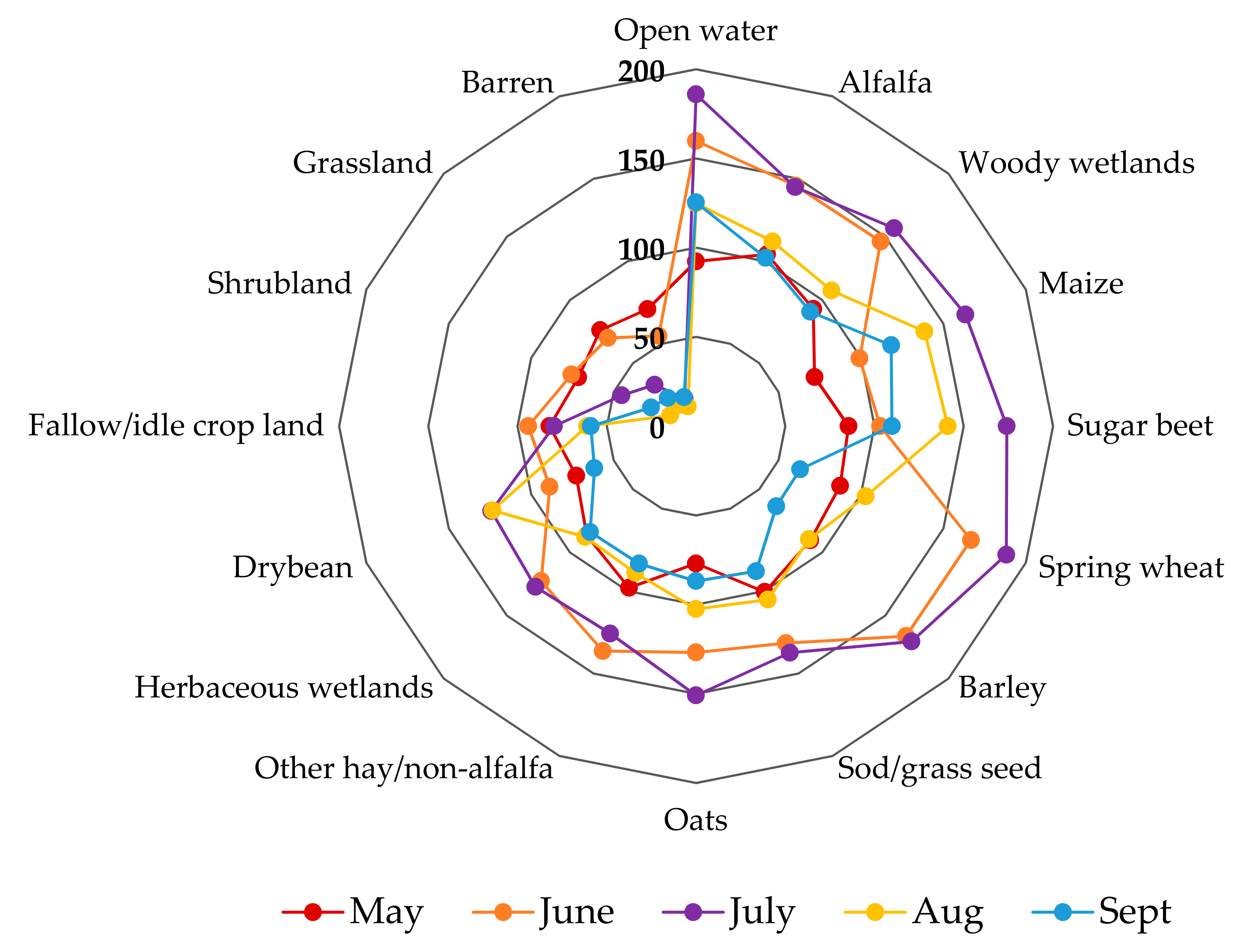
3.6. Comparison of METRIC Estimated Mean Monthly Evapotranspiration for Different Land Cover Type

Monthly ET_c is the summation of the amount of water lost from a cropped surface during each day of the month. Monthly and seasonal ET_c estimates are valuable in determining the irrigation, storage, and conveyance capacities of an irrigation system. Figure 11 shows the METRIC estimated mean monthly ET_c rate for sixteen different land cover type viz. alfalfa, dry bean, sugar beet, barley, Maize, Oats, other hay/non-alfalfa, sod/grass seed, spring wheat, fallow/idle crop, barren, open water, shrubland, grassland, woody wetlands, and herbaceous wetlands during 2018 growing season (May–September). While estimating periodic ET_c rate for each landcover type, the clouded part seen on some of the images were cropped out. The monthly ET_c estimates for crops exhibited a bell-shaped ET_c curve. This implies monthly ET_c rate will be lower during the beginning and end of the growing season and higher during mid-season when plants have good canopy cover to transpire at their potential rates. Early planting date (starts mid-March) for barley means it reached its peak growth during the period from June to July resulting in a higher ETc rate during those months. The monthly ET_c values from the barley field start decreasing by August as the crop reaches physiological maturity. The harvesting of barley starts from early August and can last until Mid-August. Monthly ET_c values observed from barley fields after harvesting accounts to surface residue ET_c and soil evaporation. Dry bean, sugar beet, and maize had the highest ET_c rate during July and August which coincides with the peak growth and flowering stage of these crops. Dry bean fields experienced lower monthly ET_c values as compared to fields of Maize and sugar beet (Figure 11). Dry bean tends to have less dense vegetation and a shorter growing span, resulting in a lower rate of cumulative ET_c. Unlike dry bean, sugar beet and maize field had considerably higher ET_c values until September. Maize and sugar beet have fair vegetation cover until September and subsequently senesce prior to harvest in October. In Wyoming, alfalfa is grown primarily for hay under irrigation. Alfalfa fields have higher ET_c values in May as compared to other crops as it is planted by early-August of the previous year and is already established by winter. Likewise, alfalfa has a longer growing season, a deep root system, and a dense canopy of vegetation that results in higher cumulative seasonal ET_c values as compared to other crops. Alfalfa is normally harvested 2–3 times a year with the most active harvesting period between June to September that results in fluctuation of monthly ET_c values during this period. As expected, the naturally vegetated areas had lower average monthly ET_c values as compared to those of crop fields.

Similarly, Figure 11 indicates open water evaporation (E_water) to be greater than wetland ET (ET_wetland) in the study area. E_water − ET_wetland was less during early (May) and late growing season (October). However, the difference increased considerably during the mid-season summer and fall images (June, July, August, and September). This increase in the difference in mid-season can be associated with vegetation senescence (resulting in low ET_wetland) in the wetland region. On the other hand, water has high specific heat and heat capacity that induces it to absorb and store thermal energy. The storage of thermal energy in the water body is greater in summer and fall as more radiant energy is available. The greater release of stored heat in summer and fall from open water increases the net energy available for evaporation. The E_water − ET_wetland value was much higher for herbaceous wetlands (E_water − ET _{herbaceous-wetland} = 33.7%) as compared to woody wetlands (E_water − ET_{woody-wetland} = 15%). Stannard et al. [68] used eddy covariance to measure ET_wetland rates from two wetland sites and BREBS to measure E_water rate from two open water sites for three years and reported overall E_water to be 20% greater than overall ET_wetland. Their study also reported E_water − ET_wetland to have a lower difference from late June to early August, while the difference increased during late summer.

The majority of the study area in this study is under natural vegetation (about 83%). A comparison was done to assess METRIC estimated surface energy balance fluxes between cropland and natural vegetation (Figure 12). For that, average flux across the study area on five different image acquisition dates comprising early (15 May), mid (8 June, 18 July, and 11 August), and late-season (12 September) during the 2018 growing season were considered. Natural vegetation had comparatively lower R_n values (up to 15% lower) as compared to cropland as the growing season progressed. The difference in the net radiation values can be associated with the variation in surface albedo value. As the growing season progresses, the bare soil in the naturally vegetated area is dry (because of water stress) and has higher albedo values (dry soil albedo was reported to be around 0.31 by Idso et al. [69]) causing a decline in R_n. However, during the early season, the soil in the natural vegetation area is wet (because of possible precipitation and snow cover) with lower albedo values (wet soil albedo was reported to be be around 0.14 by Idso et al. [69]) causing the R_n to be similar or sometimes greater than that of cropland, as evidenced in May in our study area. Natural vegetation can also have lower albedo value due to the effect of shading that might happen in taller vegetation like forest and woody wetlands. As compared to cropland, naturally vegetated areas had higher H value (up to 94% higher in mid-season). A huge proportion of R_n energy is used up by crops in the ET_c process, thus lowering the H and G estimates in cropland. Natural vegetation, on the other hand, have a lower ET_c rate, and the net available energy is partitioned more into H and G. Lower H values in cropland during mid-season indicate crops transpiring at a higher rate whereas higher sensible heat values for crops at the end and beginning of growing season indicate lowering ET_c rate. Higher ET_c rate in the early season lowered the H value whereas lower ET_c rate during the mid-season resulted in a higher H. Lower H values at the end of the growing season is caused by the decline in net available radiant energy [58]. G has a reciprocal relationship with high ground cover (shading or insulation effect) and leaf area index and a direct proportional relationship with albedo. These factors cause a significant difference between crop land and natural vegetation G. The decreasing G value at the end of the growing season in the natural vegetation area reflects less availability of R_n energy. During the early season, the ET_c rate from the cropland can be similar or in some cases less than that of natural vegetation as evidenced during the month of May in this study. The precipitation received early in the growing season helps natural vegetation induce new growth and thus transpire more. However, as the season progresses, the natural vegetation could suffer from water stress, resulting in a lower ET_c rate as compared to that of cropland, where P gets accompanied by irrigation.

3.7. Irrigation District Average Water Consumption

One of the main objectives of this study is to use satellite estimated ET_c to quantify the average crop water use and crop water use for different cropping systems for different irrigation districts within the study area.

Table 4. Average crop evapotranspiration (ET_c), seasonal precipitation (P), and percent of irrigation-based ET_c for 2017 and 2018 crop growing season over nine irrigation districts in the study region.

	Irrigation District	Year	Avg. ETc (mm)	A (km2)	Area Wise Total ETc (km3)	P (mm)	Area Wise Total P (km3)	Irrigation (ETc-P) (km3)	% of Irrigation Contributing to ETc
1	Cody Canal	2017	699	157	0.11	158	0.02	0.08	77
		2018	653	157	0.10	204	0.03	0.07	69
2	Deaver	2017	666	277	0.18	117	0.03	0.15	82
		2018	610	277	0.17	158	0.04	0.13	74
3	Greybull Valley	2017	609	1284	0.78	125	0.16	0.62	79
		2018	587	1284	0.75	162	0.21	0.54	72
4	Heart Mountain	2017	713	584	0.42	146	0.09	0.33	80
		2018	665	584	0.39	197	0.11	0.27	70
5	Hunt & Godfrey	2017	717	51	0.04	124	0.01	0.03	83
		2018	658	51	0.03	177	0.01	0.02	73
6	Lovell	2017	678	30	0.02	121	0.00	0.02	82
		2018	658	30	0.02	164	0.00	0.01	75
7	Shoshone	2017	620	538	0.33	125	0.07	0.27	80
		2018	606	538	0.33	167	0.09	0.24	72
8	Sidon	2017	637	207	0.13	121	0.03	0.11	81
		2018	628	207	0.13	151	0.03	0.10	76
9	Willwood	2017	642	196	0.13	124	0.02	0.10	81
		2018	673	196	0.13	153	0.03	0.10	77

presents the average ET_c, P, and percent of irrigation-based ET_c for 2017 and 2018 crop growing seasons over nine irrigation districts in the study region. For this analysis, monthly P values for 2017 and 2018 for each irrigation district were extracted from gridded 4-km monthly parameter-elevation regression on independent slope model (PRISM) dataset [70] obtained from the PRISM Climate Group website. Within the study region, the area of each irrigation district varies from 51 Km² for the Hunt and Godfrey irrigation district to 1284 Km² for the Greybull Valley irrigation district. No significant difference was observed in seasonal crop ET_c among the irrigation districts, with average ET_c (average of two years) ranging from 598 mm in Greybull Irrigation District to 689 mm in Heart Mountain irrigation district. The seasonal ET_c for 2017 was approximately 34 mm greater than 2018, except for the Will Wood irrigation district where greater ET_c was observed for 2018. This may be due to higher precipitation P and lower T_air in 2018 where average precipitation P was 19 mm higher than 2017 and average T_air was 0.50 °C lower than 2017. To understand the amount of ET contributed by irrigation, irrigation volumes for each irrigation district were calculated by subtracting the average seasonal P from ET_c (ET_c − P) for each irrigation district, assuming other variables such as streamflow and change in soil moisture are negligible. This assumption is valid considering the semi-arid to arid intermountain region of Wyoming, where seasonal precipitation is generally less than 200 mm. The results indicated that, in 2017, an average of 81% (maximum of 83% in Hunt and Godfrey irrigation district and minimum of 79% in Greybull irrigation district) and, in 2018, an average of 73% (maximum of 77% and minimum of 69%) of ET_c is contributed by irrigation only.

To further understand the dynamics of seasonal ETc from different vegetative surfaces, ET_c and percent irrigation contribution to ET_c for four major crop types within each irrigation district were analyzed (refer Supplementary Materials, Tables S1–S9). For both years, higher ET_c was observed for alfalfa followed by sugar beet, and the lowest ET_c was observed for dry bean in all irrigation districts. The percent irrigation contribution to ET_c (ET_c-P) varies from 60% for dry beans in the Heart Mountain irrigation district in 2018 to a maximum of 83% for alfalfa in Lovell and Deaver irrigation districts in 2017. This information could be very useful for irrigation district personnel, water managers, decision-makers, policymakers, and state and federal water regulatory agencies for quantification/re-evaluation of the overall distribution of evaporative losses for a given irrigation district relative to available water resources for evaluating various management practices.

4. Summary and Conclusions

Estimates of ET_c represent a key component of water management in croplands, naturally vegetated areas, open water sources, wetlands, and riparian basins. Today, determining short term and long term ET_c rates to guide water resource-based policy and decision making has become a necessity. In the face of population increment and water scarcity around the globe, the importance of ET_c has grown many folds. A total of 22 cloud-free Landsat 7-ETM+ and Landsat 8–OLI and TIRS images were analyzed using a satellite-based energy balance model, namely mapping evapotranspiration with internalized calibration (METRIC). The study was carried out for 2017, 2018, and 2019 growing season period in the semi-arid to arid intermountain region of Wyoming (Path/Row: 37/29). The accuracy check of METRIC estimates was done by comparing estimated instantaneous and periodic fluxes with respective Bowen ratio energy balance system (BREBS) measured fluxes. The BREBS station was installed on a center pivot irrigation field and had sugar beet in 2017, dry beans in 2018, and barley in 2019 growing season. The correlation observed between estimated and measured instantaneous energy balance fluxes (pooled data points) had R² values of 0.91 (RMSE = 0.08 mm h⁻¹, NSE = 0.91), 0.81 (RMSE = 49.6 W m⁻², NSE = 0.67), 0.53 (RMSE = 27.1 W m⁻², NSE = 0.53), and 0.86 (RMSE = 59.2 W m⁻², NSE = 0.84) for ET_c, R_n, G, and H respectively. Likewise, estimated instantaneous energy balance fluxes (pooled data points considered) differed with BREBS fluxes by 5.7%, 5.8%, −0.8%, and 12.6% for ET_c, R_n, G, and H, respectively. Cubic spline interpolation performed a bit better as compared to linear interpolation, and a comparison of estimated and measured monthly ET_c values (pooled data) for cubic spline had R² and slope of 0.9 and RMSE of 18.3 mm with growing season ET_c underestimated in the range between 3.2 to 6.02%. A spatio-temporal distribution maps of instantaneous energy balance fluxes and seasonal ET_c showed an anticipated variation across the study area as the plant growth stage and surface condition changed. In addition, mean monthly ET_c values estimated across the study area for different land cover types showed a substantial variation throughout the growing season as climate and crop growth stages differed. Furthermore, it was found that, in the arid to semi-arid intermountain region of Wyoming, the contribution of irrigation varied in the range of 73–81% of the total seasonal ET_c in nine irrigation districts that fall within the study area. The high relative contribution of irrigation highlights the importance of identifying and quantifying ET_c for improved management in irrigation system design and water allocation.

In this study, METRIC algorithms performed reasonably well, particularly in estimating cumulative ET_c for the entire growing season. However, the model performance was poor during the early and late growing season when fields had little active leaf area, with METRIC estimated ET_c values were within 10% of the BREBS measured values. A companion paper to the research compared the performance of four surface energy balance models viz. METRIC, SEBAL, SEBS, and S-SEBI in estimating the ETc in the intermountain region of Wyoming. The METRIC model can be an important tool in quantifying and mapping surface energy balance components especially in places where quality hourly weather data are available. Accurate hot and cold pixel selection during sensible heat calculation is a defining moment of the METRIC algorithm. A selection error can result in an undesired outcome. The selection of hot pixels was an arduous task, especially when P events occurred prior to Landsat overpass time, raising the LE value. Similarly, the estimation of negative reference ET fraction (ET_rF) in some naturally vegetated and deserted areas was observed altering ET_c estimation for those surfaces. Thus, further research work on securing accurate hot pixels during prior P events, controlling wayward estimations during the early and late growing season, and minimizing the estimation of negative reference ET fraction in naturally vegetated and deserted areas can provide important support for a more accurate estimation of instantaneous and periodic fluxes. Furthermore, future research will also focus on multi-sensor data fusion to increase the temporal variation and thereby reduce the uncertainties in ET_c estimations.

References

1. Sharma, V.; Nicholson, C.; Bergantino, A.; Irmak, S.; Peck, D. Temporal Trend Analysis of Meteorological Variables and Reference Evapotranspiration in the Inter-mountain Region of Wyoming. Water 2020, 12, 2159. [Google Scholar] [CrossRef]
2. United States Department of Agriculture. Census of Agriculture. Available online: https://www.nass.usda.gov/Publications/AgCensus/2012/Full_Report/Volume_1,_Chapter_1_State_Level/ (accessed on 14 July 2020).
3. Jacobs, J.J.; Brosz, D.J. Wyoming Water Law: A Summary; Bulletin B-969; C; Cooperative Extension Service, College of Agriculture and Wyoming Water Research Center, University of Wyoming: Laramie, WY, USA, 1993. [Google Scholar]
4. Hansen, K.; Nicholson, C.M.; Paige, G. Wyoming’s Water: Resources & Management; University of Wyoming Extension: Laramie, WY, USA, 2015. [Google Scholar]
5. Irmak, S. Nebraska Water and Energy Flux Measurement, Modeling, and Research Network (NEBFLUX). Trans. ASABE 2010, 53, 1097–1115. [Google Scholar] [CrossRef]
6. Gowda, P.H.; Chavez, J.L.; Colaizzi, P.D.; Evett, S.R.; Howell, T.A.; Tolk, J.A. ET mapping for agricultural water management: Present status and challenges. Irrig. Sci. 2008, 26, 223–237. [Google Scholar] [CrossRef] [Green Version]
7. Wagle, P.; Gowda, P.H. Editorial for the Special Issue “Remote Sensing of Evapotranspiration (ET)”. Remote Sens. 2019, 11, 2146. [Google Scholar] [CrossRef] [Green Version]
8. Sharma, V.; Irmak, S. Mapping spatially interpolated precipitation, reference evapotranspiration, actual crop evapotranspiration, and net irrigation requirements in Nebraska: Part II. Actual crop evapotranspiration and net irrigation requirements. Trans. ASABE 2012, 55, 907–921. [Google Scholar] [CrossRef]
9. Allen, R.G.; Tasumi, M.; Morse, A.T.; Trezza, R. A Landsat-based energy balance and evapotranspiration model in Western US water rights regulation and planning. Irrig. Drain. Syst. 2005, 19, 251–268. [Google Scholar] [CrossRef]
10. Allen, R.G.; Pereira, L.S.; Raes, D.; Smith, M. FAO Irrigation and Drainage Paper No. 56: Crop Evapotranspiration; FAO: Rome, Italy, 1998. [Google Scholar]
11. Moorhead, J.E.; Marek, G.W.; Gowda, P.H.; Lin, X.; Colaizzi, P.D.; Evett, S.R.; Kutikoff, S. Evaluation of Evapotranspiration from Eddy Covariance Using Large Weighing Lysimeters. Agronomy 2019, 9, 99. [Google Scholar] [CrossRef] [Green Version]
12. Howell, T.A.; Schneider, A.D.; Jensen, M.E. History of Lysimeter Design and Use for Evapotranspiration Measurements. In Proceedings of the Lysimeters for Evapotranspiration and Environmental Measurements, Honolulu, HI, USA, 23–25 July 1991; pp. 1–9. [Google Scholar]
13. Sharma, V.; Kilic, A.; Irmak, S. Impact of scale/resolution on evapotranspiration from Landsat and MODIS images. Water Resour. Res. 2016, 52, 1800–1819. [Google Scholar] [CrossRef] [Green Version]
14. Su, Z. The surface energy balance system (SEBS) for estimation of turbulent heat fluxes. Hydrol. Earth Syst. Sci. 2002, 6, 85–99. [Google Scholar] [CrossRef]
15. Bastiaanssen, W.G.M.; Menenti, M.; Feddes, R.A.; Holtslag, A.A.M. A remote sensing surface energy balance algorithm for land (SEBAL): 1. Formulation. J. Hydrol. 1998, 212, 198–212. [Google Scholar] [CrossRef]
16. Meneti, M.; Choudhary, B.J. Parameterization of land surface evapotranspiration using a location dependent potential evapotranspiration and surface temperature range. Exch. Process. Land Surf. A Range Space Time Scales 1993, 212, 561–568. [Google Scholar]
17. Roerink, G.J.; Su, Z.; Menenti, M. S-SEBI: A simple remote sensing algorithm to estimate the surface energy balance. Phys. Chem. Earth Part B 2000, 25, 147–157. [Google Scholar] [CrossRef]
18. Senay, G.B.; Bohms, S.; Singh, R.K.; Gowda, P.H.; Velpuri, N.M.; Alemu, H.; Verdin, J.P. Operational evapotranspiration mapping using remote sensing and weather datasets—A new parameterization for the SSEB approach. J. Am. Water Resour. Assoc. 2013, 49, 577–591. [Google Scholar] [CrossRef] [Green Version]
19. Allen, R.G.; Tasumi, M.; Morse, A.T.; Trezza, R.; Wright, J.L.; Bastiaanssen, W.; Kramber, W.; Lorite, I.; Robison, C.W. Satellite-based energy balance for mapping evapotranspiration with internalized calibration (METRIC)- Applications. J. Irrig. Drain. Eng. 2007, 133, 395–406. [Google Scholar] [CrossRef]
20. Allen, R.G.; Tasumi, M.; Trezza, R. Satellite-based energy balance for mapping evapotranspiration with internalized calibration (METRIC)-Model. J. Irrig. Drain. Eng. 2007, 133, 380–394. [Google Scholar] [CrossRef]
21. Bastiaanssen, W.G.M. Regionalization of Surface Flux Densities and Moisture Indicators in Composite Terrain: A Remote Sensing Approach under Clear Skies in Mediterranean Climates. Ph.D. Thesis, CIP Data Koninklijke Bibliotheek, Den Haag, The Netherlands, 1995. [Google Scholar]
22. Bastiaanssen, W.G.M. SEBAL-based sensible and latent heat fluxes in the irrigated Gediz Basin, Turkey. J. Hydrol. 2000, 229, 87–100. [Google Scholar] [CrossRef]
23. Bastiaanssen, W.G.M.; Pelgrum, H.; Wang, J.; Ma, Y.; Moreno, J.; Roerink, G.J.; van der Wal, T. The surface energy balance algorithm for land (SEBAL): 2. Validation. J. Hydrol. 1998, 212, 213–229. [Google Scholar] [CrossRef]
24. Bastiaanssen, W.G.M.; Noordman, E.J.M.; Pelgrum, H.; Thoreson, B.P.; Allen, R.G. SEBAL model with remotely sensed data to improve water-resources management under actual field conditions. J. Irrig. Drain. Eng. 2005, 131, 85–93. [Google Scholar] [CrossRef]
25. Tasumi, M.; Trezza, R.; Allen, R.G.; Wright, J.L. Operational aspects of satellite-based energy balance models for irrigated crops in the semi-arid US. Irrig. Drain. Syst. 2005, 19, 355–376. [Google Scholar] [CrossRef]
26. Trezza, R.; Allen, R.G.; Tasumi, M. Estimation of actual evapotranspiration along the Middle Rio Grande of New Mexico Using MODIS and landsat imagery with the METRIC model. Remote Sens. 2013, 5, 5397–5423. [Google Scholar] [CrossRef] [Green Version]
27. French, A.N.; Hunsaker, D.J.; Thorp, K.R. Remote sensing of evapotranspiration over cotton using the TSEB and METRIC energy balance models. Remote Sens. Environ. 2015, 158, 281–294. [Google Scholar] [CrossRef]
28. Dhungel, R.; Allen, R.G.; Trezza, R.; Robison, C.W. Evapotranspiration between satellite overpasses: Methodology and case study in agricultural dominant semi-arid areas. Meteorol. Appl. 2016, 23, 714–730. [Google Scholar] [CrossRef]
29. Numata, I.; Khand, K.; Kjaersgaard, J.; Cochrane, M.A.; Silva, S.S. Evaluation of landsat-based METRIC modeling to provide high-spatial resolution evapotranspiration estimates for amazonian forests. Remote Sens. 2017, 9, 46. [Google Scholar] [CrossRef] [Green Version]
30. Khand, K.; Kjaersgaard, J.; Hay, C.; Jia, X. Estimating Impacts of Agricultural Subsurface Drainage on Evapotranspiration Using the Landsat Imagery-Based METRIC Model. Hydrology 2017, 4, 49. [Google Scholar] [CrossRef] [Green Version]
31. Gowda, P.H.; Chávez, J.L.; Howell, T.A.; Marek, T.; New, L.L. Surface Energy Balance Based Evapotranspiration Mapping in the Texas High Plains. Sensors 2008, 8, 5186–5201. [Google Scholar] [CrossRef]
32. Madugundu, R.; Al-Gaadi, K.A.; Tola, E.K.; Hassaballa, A.A.; Patil, V.C. Performance of the METRIC model in estimating evapotranspiration fluxes over an irrigated field in Saudi Arabia using Landsat-8 images. Hydrol. Earth Syst. Sci. 2017, 21, 6135–6151. [Google Scholar] [CrossRef] [Green Version]
33. Tasumi, M. Estimating evapotranspiration using METRIC model and Landsat data for better understandings of regional hydrology in the western Urmia Lake Basin. Agric. Water Manag. 2019, 226. [Google Scholar] [CrossRef]
34. Singh, R.K.; Senay, G.B. Comparison of Four Different Energy Balance Models for Estimating Evapotranspiration in the Midwestern United States. Water 2015, 8, 9. [Google Scholar] [CrossRef] [Green Version]
35. Singh, R.K.; Liu, S.; Tieszen, L.L.; Suyker, A.E.; Verma, S.B. Estimating seasonal evapotranspiration from temporal satellite images. Irrig. Sci. 2012, 30, 303–313. [Google Scholar] [CrossRef] [Green Version]
36. Mokhtari, M.H.; Ahmad, B.B.; Hoveidi, H.; Busu, I. Sensitivity Analysis of METRIC-Based Evapotranspiration Algorithm. Int. J. Environ. Res. 2013, 7, 407–422. [Google Scholar] [CrossRef]
37. Tang, Q.; Peterson, S.; Cuenca, R.H.; Hagimoto, Y.; Lettenmaier, D.P. Satellite-based near-real-time estimation of irrigated crop water consumption. J. Geophys. Res. 2009, 114. [Google Scholar] [CrossRef]
38. De la Fuente-Sáiz, D.; Ortega-Farías, S.; Fonseca, D.; Ortega-Salazar, S.; Kilic, A.; Allen, R. Calibration of METRIC Model to Estimate Energy Balance over a Drip-Irrigated Apple Orchard. Remote Sens. 2017, 9, 670. [Google Scholar] [CrossRef] [Green Version]
39. Pôças, I.; Paço, T.A.; Cunha, M.; Andrade, J.A.; Silvestre, J.; Sousa, A.; Santos, F.L.; Pereira, L.S.; Allen, R.G. Satellite-based evapotranspiration of a super intensive olive orchard: Application of METRIC algorithms. Biosyst. Eng. 2014, 128, 69–81. [Google Scholar] [CrossRef] [Green Version]
40. Paço, T.A.; Pôças, I.; Cunha, M.; Silvestre, J.C.; Santos, F.L.; Paredes, P.; Pereira, L.S. Evapotranspiration and crop coefficients for a super intensive olive orchard. An application of SIMDualKc and METRIC models using ground and satellite observations. J. Hydrol. 2014, 519, 2067–2080. [Google Scholar] [CrossRef] [Green Version]
41. Allen, R.G.; Irmak, A.; Trezza, R.; Hendrickx, J.; Bastiaanssen, W. Satellite Based ET Estimation in Agriculture using SEBAL and METRIC. J. Hydrol. Process. 2011, 25, 4011–4027. [Google Scholar] [CrossRef]
42. National Oceanic and Atmospheric Administration. Climate at a Glance. Available online: https://www.ncdc.noaa.gov/cag/national/rankings (accessed on 3 March 2020).
43. Sharma, V.; Nicholson, C.; Bergantino, T.; Cowley, J.; Hess, B.; Tanaka, J. Wyoming Agricultural Climate Network (WACNet). In Agricultural Experiment Station 2018 Field Days Bulletin; University of Wyoming: Laramie, WY, USA, 2018; pp. 52–53. [Google Scholar]
44. Fritschen, L.J. Evapotranspiration Rates of Field Crops Determined by the Bowen Ratio Method. Agron. J. 1966, 58, 339–342. [Google Scholar] [CrossRef]
45. Huete, A.R.; Jackson, R.D.; Post, D.F. Spectral response of a plant canopy with different soil backgrounds. Remote Sens. Environ. 1985, 17, 37–53. [Google Scholar] [CrossRef]
46. Huete, A.R. A Soil-Adjusted Vegetation Index (SAVI). Remote Sens. Environ. 1988, 25, 295–309. [Google Scholar] [CrossRef]
47. Duffie, J.A.; Beckman, W.A. Solar Engineering of Thermal Processes, 2nd ed.; John Wiley and Sons: New York, NY, USA, 1991. [Google Scholar]
48. Starks, P.J.; Norman, J.M.; Blad, B.L.; Walter-Shea, E.A.; Walthall, C.L. Estimation of shortwave hemispherical reflectance (albedo) from bidirectionally reflected radiance data. Remote Sens. Environ. 1991, 38, 123–134. [Google Scholar] [CrossRef]
49. Tasumi, M.; Allen, R.G.; Trezza, R. At-surface albedo from Landsat and MODIS satellites for use in energy balance studies of evapotranspiration. J. Hydrol. Eng. 2008, 13, 51–63. [Google Scholar] [CrossRef]
50. Olmedo, G.F.; Ortega-Farías, S.; Fuente-Sáiz, D.; Fonseca-Luego, D.; Fuentes-Peñailillo, F. Water: Tools and Functions to Estimate Actual Evapotranspiration Using Land Surface Energy Balance Models in R. R J. 2016, 8, 352–369. [Google Scholar] [CrossRef] [Green Version]
51. Tasumi, M. Progress in Operational Estimation of Regional Evapotranspiration Using Satellite Imagery. Ph.D. Thesis, University of Idaho, Moscow, ID, USA, 2003. [Google Scholar]
52. Tasumi, M.; Allen, R.G.; Trezza, R.; Wright, J.L. Satellite-based energy balance to assess within population variance of crop coefficient curves. J. Irrig. Drain. Eng. 2005, 131, 94–109. [Google Scholar] [CrossRef]
53. ASCE-EWRI. The ASCE standardized reference evapotranspiration equation. In ASCE-EWRI Standardization of Reference Evapotranspiration Task Committee Report; ASCE Bookstore: Reston, VA, USA, 2005. [Google Scholar]
54. Romero, M.G. Daily Evapotranspiration Estimation by Means of Evaporative Fraction and Reference ET Fraction. Ph.D. Thesis, Utah State University, Logan, UT, USA, 2004. [Google Scholar]
55. Singh, R.K.; Irmak, A. Estimation of crop coefficient using satellite remote sensing. J. Irrig. Drain. Eng. 2009, 135, 597–608. [Google Scholar] [CrossRef]
56. Wright, J.L. New Evapotranspiration Crop Coefficients. J. Irrig. Drain. Div. 1982, 108, 57–74. [Google Scholar]
57. Horton, R.; Bristow, K.L.; Kluitenberg, G.; Sauer, T.J. Crop residue effects on surface radiation and energy balance: Review. Theor. Appl. Climatol. 1996, 54, 27–37. [Google Scholar] [CrossRef] [Green Version]
58. Sharma, V.; Irmak, S.; Kilic, A.; Mutiibwa, D. Application of remote sensing for quantifying and mapping surface energy fluxes in south central Nebraska: Analyses with respect to field measurements. Trans. ASABE 2015, 58, 1265–1285. [Google Scholar]
59. Mu, Q.; Jones, L.A.; Kimball, J.S.; McDonald, K.C.; Running, S.W. Satellite assessment of land surface evapotranspiration for the pan-Arctic domain. Water Resour. Res. 2009, 45. [Google Scholar] [CrossRef] [Green Version]
60. Kilic, A.; Ratcliffe, I.; Ranade, P.; Hubbard, K.; Singh, R.K.; Kamble, B.; Kjaersgaard, J. Estimation of Land Surface Evapotranspiration with a Satellite Remote Sensing Procedure. Great Plains Res. J. Nat. Soc. Sci. 2011, 21, 73–88. [Google Scholar]
61. Irmak, A.; Singh, R.; Walter-Shea, E.A.; Verma, S.; Suyker, A.E. Comparison and analysis of empirical equations for soil heat flux for different cropping systems and irrigation methods. Trans. ASABE 2011, 53, 67–80. [Google Scholar] [CrossRef] [Green Version]
62. Barr, A.G.; King, K.M.; Gillespie, T.J.; Hartog, G.D.; Neumann, H.H. A comparison of bowen ratio and eddy correlation sensible and latent heat flux measurements above deciduous forest. Bound. Layer Meteorol. 1994, 71, 21–41. [Google Scholar] [CrossRef]
63. McBean, G.A. Role of Active-Passive Scalar Relationships in Evaporation from Vegetated Surfaces. In Advances in Theoretical Hydrology; O’Kane, J.R., Ed.; Elsevier Science: Amsterdam, The Netherlands, 1992; pp. 47–58. [Google Scholar]
64. Monteith, J.L. Dew. Q. J. R. Meteorol. Soc. 1957, 83, 322–341. [Google Scholar] [CrossRef]
65. Sharma, M.L. Contribution of dew in the hydrologic balance of semi-arid grassland. Agric. Meteorol. 1976, 17, 321–331. [Google Scholar] [CrossRef]
66. National Oceanic and Atmospheric Administration. National Weather Service. Available online: https://www.weather.gov/cle/seasons (accessed on 2 August 2020).
67. McGowan, H.A.; Sturman, A.P.; Mackellar, M.C.; Weibe, A.H.; Neil, D.T. Measurements of the local energy balance over a coral reef flat, Heron Island, southern Great Barrier Reef, Australia. J. Geophys. Res. 2010, 115. [Google Scholar] [CrossRef] [Green Version]
68. Stannard, D.I.; Gannett, M.W.; Polette, D.J.; Cameron, J.M.; Waibel, M.S.; Spears, J.M. Evapotranspiration from wetland and open-water sites at Upper Klamath Lake, Oregon, 2008–2010. In Scientific Investigations Report; U.S. Geological Survey: Reston, VA, USA, 2013; p. 66. [Google Scholar]
69. Idso, S.B.; Jackson, R.D.; Reginato, R.J.; Kimball, B.A.; Nakayama, F.S. The Dependence of Bare soil albedo on soil water content. J. Appl. Meteorol. Climatol. 1975, 14, 109–113. [Google Scholar] [CrossRef] [Green Version]
70. Daly, C.; Halbleib, M.; Smith, J.I.; Gibson, W.P.; Doggett, M.K.; Taylor, G.H.; Curtis, J.; Pasteris, P.P. Physiographically sensitive mapping of cliumatological temperature and precipitation across the conterminous United States. Int. J. Climatol. 2007, 28, 2031–2064. [Google Scholar] [CrossRef]
Figure 1. Location map of the study area within the Big Horn Basin (BHB) Wyoming (a) Landsat Path 37 Row 29 footprint along with county map and location of Bowen Ratio Energy Balance System (BREBS) (b) Land use map with irrigation district boundaries of nine irrigation districts within the study area (c) elevation (meters) with hill shade effect underneath (meters).
Remotesensing 12 04019 g001
Figure 2. Bowen Ratio Energy Balance System (BREBS) installed in center pivot irrigated (a) sugar beet, (b) dry bean, and (c) barley field at Powell Research and Extension Center in Powell, Wyoming.
Remotesensing 12 04019 g002
Figure 3. Flowchart illustrating the computation of surface energy balance fluxes using METRIC algorithm.
Remotesensing 12 04019 g003
Figure 4. A plot of Surface temperature vs (a) NDVI, (b) LAI, and (c) albedo to depict the hot and cold pixel selection procedure.
Remotesensing 12 04019 g004
Figure 5. Daily and cumulative seasonal (May to September) (a) precipitation (P) and (b) reference evapotranspiration (ETr) during 2017, 2018, and 2019 at Powell Research and Extension Center, Powell, WY.
Remotesensing 12 04019 g005
Figure 6. METRIC—estimated and BREBS—measured instantaneous surface energy balance fluxes (a) crop evapotranspiration (ETc), (b) net radiation (Rn), (c) sensible heat (H), and (d) soil heat (G) for 2017, 2018, and 2019 growing season as well as a combined pooled data at the BREBS flux-tower footprint located in Powell Research and Extension Center, Powell, WY, USA.
Remotesensing 12 04019 g006
Figure 7. Comparison of METRIC estimated and BREBS station measured monthly ETc (mm) during 2017, 2018, 2019, and pooled data from all the growing seasons. (a) Linear Interpolation, (b) Cubic spline interpolation.
Remotesensing 12 04019 g007
Figure 8. Spatio-temporal distribution of METRIC estimated instantaneous net Radiation (Rn, W m−2) (ad), sensible heat (H, W m−2) (eh) and soil heat (G, W m−2) (il) on 15 May 2018, 2 July 2018, 11 August 2018 and 12 September 2018. The Black circled portion in some images represent the cloud coverage.
Remotesensing 12 04019 g008
Figure 9. Spatio-temporal distribution of METRIC estimated daily Evapotranspiration (ETc, mm d−1) during 2017 and 2018 growing season. (a) 4 May 2017, (b) 5 June 2017, (c) 21 June 2017, (d) 15 July 2017, (e) 31 July 2017, (f) 16 August 2017, (g) 1 September 2017, (h) 9 September 2017, (i) 15 May 2018, (j) 8 June 2018, (k) 2 July 2018, (l) 18 July 2018, (m) 26 July 2018, (n) 11 August 2018, (o) 4 September 2018, and (p) 12 September 2018. The Black circled portion in some images represent the cloud coverage.
Remotesensing 12 04019 g009
Figure 10. Spatio-temporal distribution of METRIC estimated seasonal ETc (mm) during (a) 2017 and (b) 2018 growing season (May–September).
Remotesensing 12 04019 g010
Figure 11. METRIC estimated mean monthly crop evapotranspiration (ETc, mm) across the study area during the 2018 growing season (May to September) for different land cover types.
Remotesensing 12 04019 g011
Figure 12. Comparison of METRIC estimated surface energy balance fluxes between cropland and natural vegetation across the study area during the 2018 growing season.
Remotesensing 12 04019 g012