Multidimensional Assessment of Food Provisioning Ecosystem Services Using Remote Sensing and Agricultural Statistics


Abstract

1. Introduction
2. Materials and Methods
2.1. Study Area
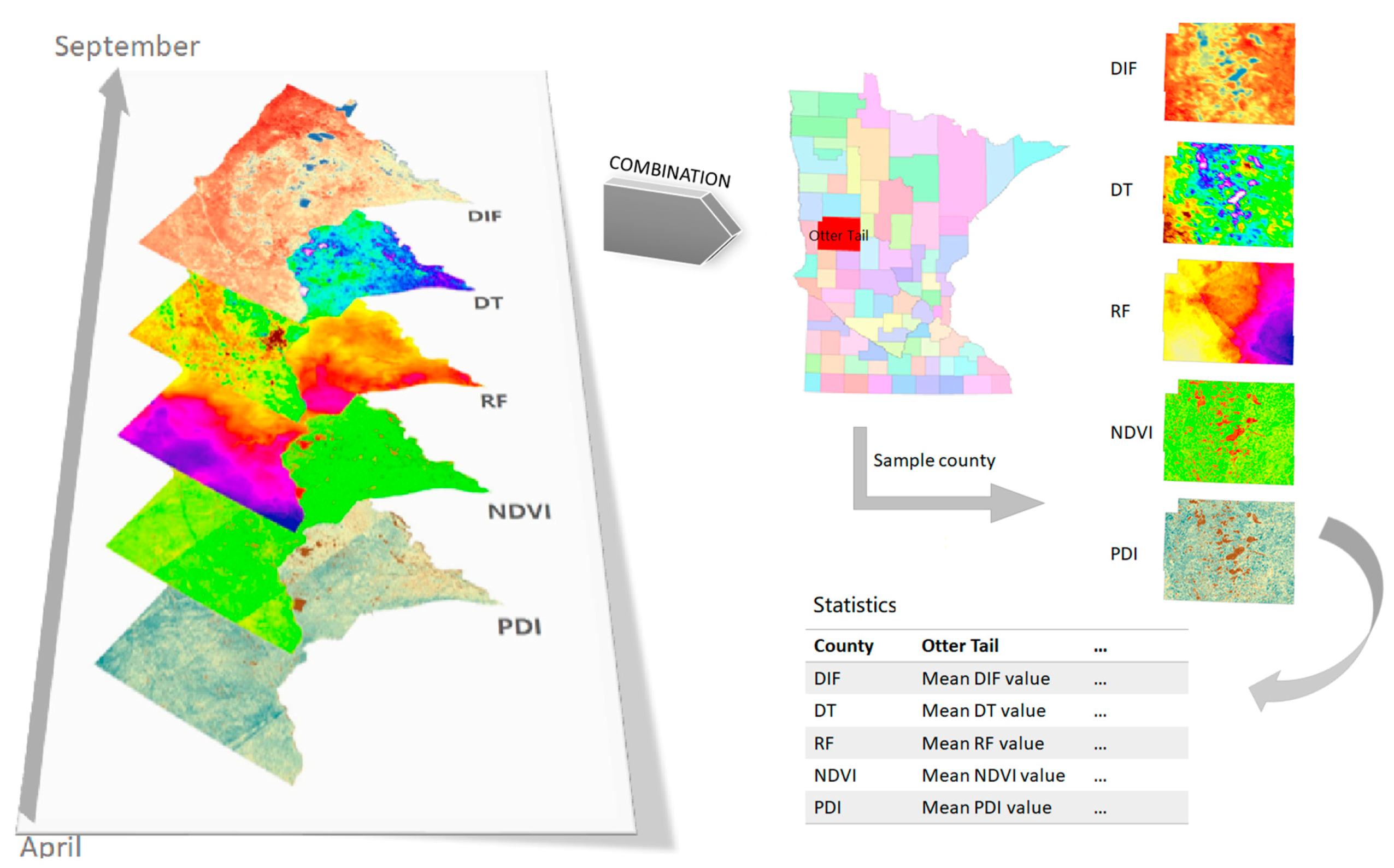
2.2. Data Sources
2.3. Methods
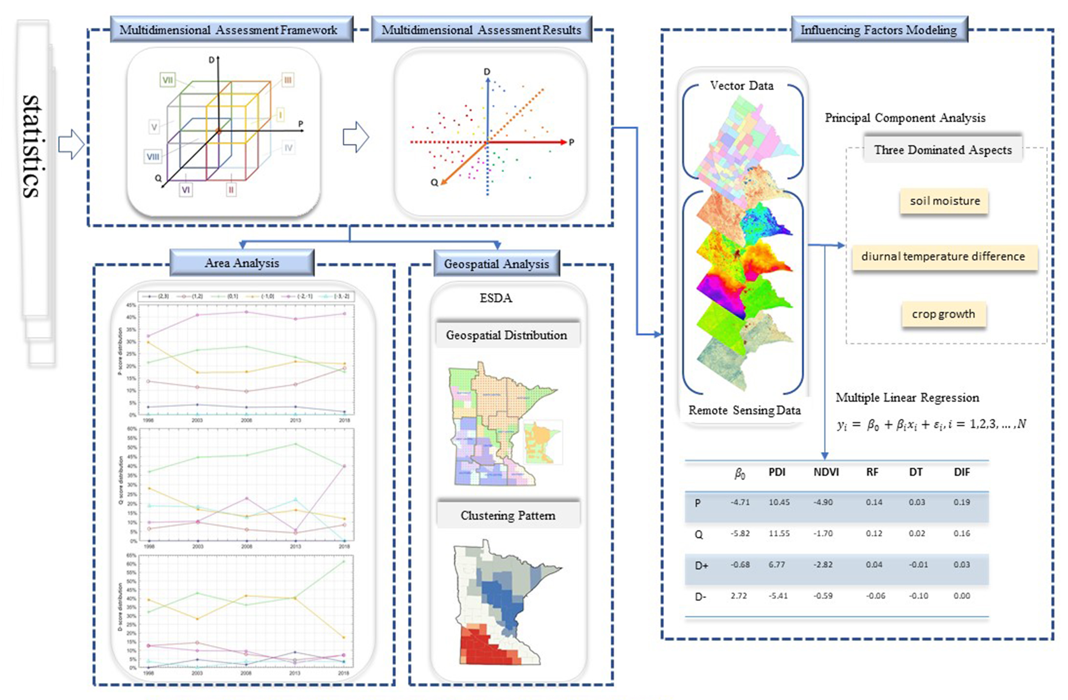
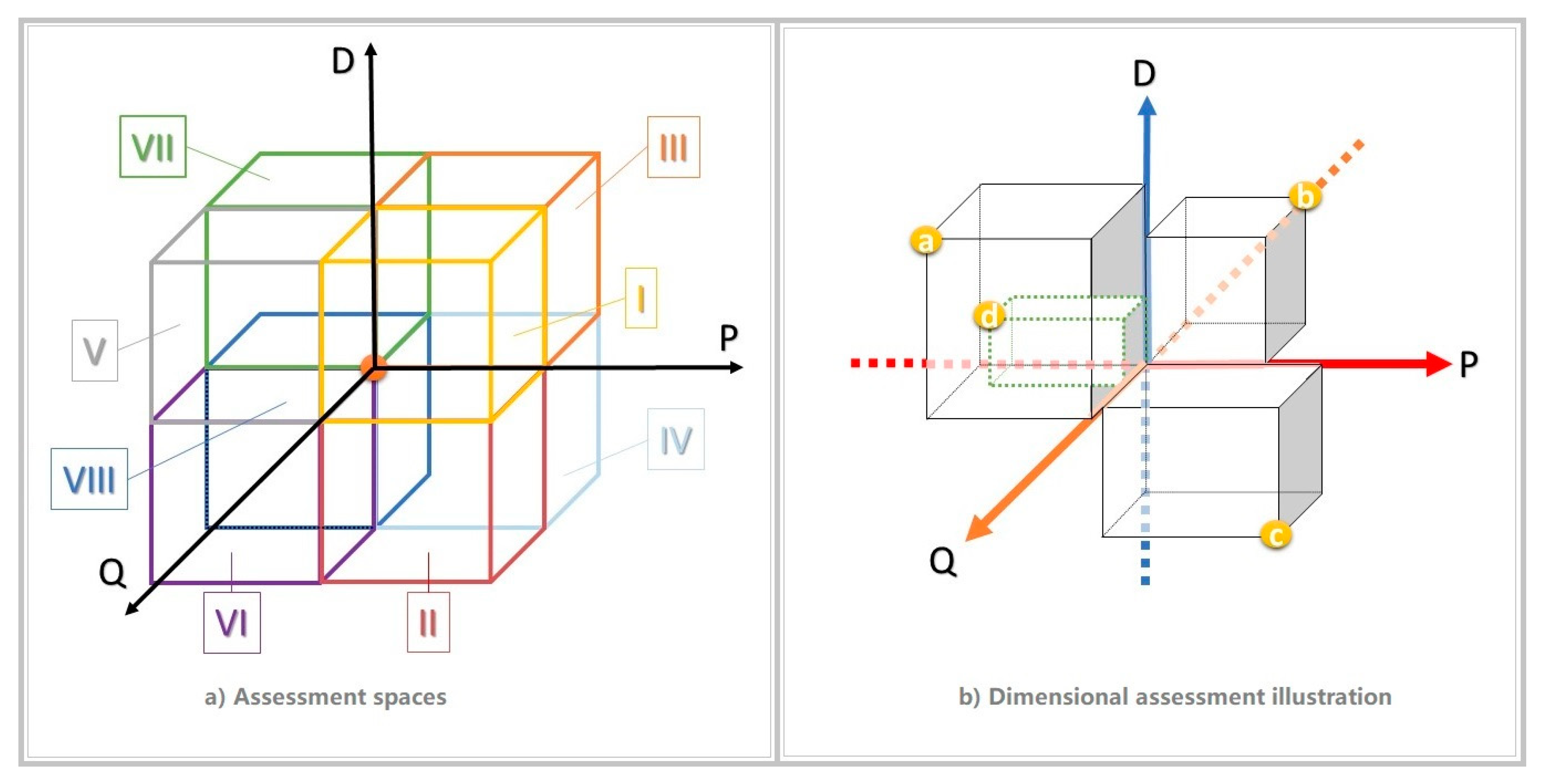
2.3.1. A Multidimensional Assessment Framework
- It is a relative assessment framework based on the average level. P-score, Q-score, and D-score are normalized to (−3,3). A positive index means an above-average dimension; the larger the index, the better the circumstance. Conversely, a negative index indicates a subaverage dimension; the lower the index is, the worse the circumstance is.
- P-score, Q-score, and D-score uniquely determine the characteristics of each county. The volume of the assessment cuboid reflects the strength of the characteristics it shows.
2.3.2. Exploratory Spatial Data Analysis
2.3.3. Remote Sensing Image Analysis
2.3.4. Statistical Analysis
3. Results
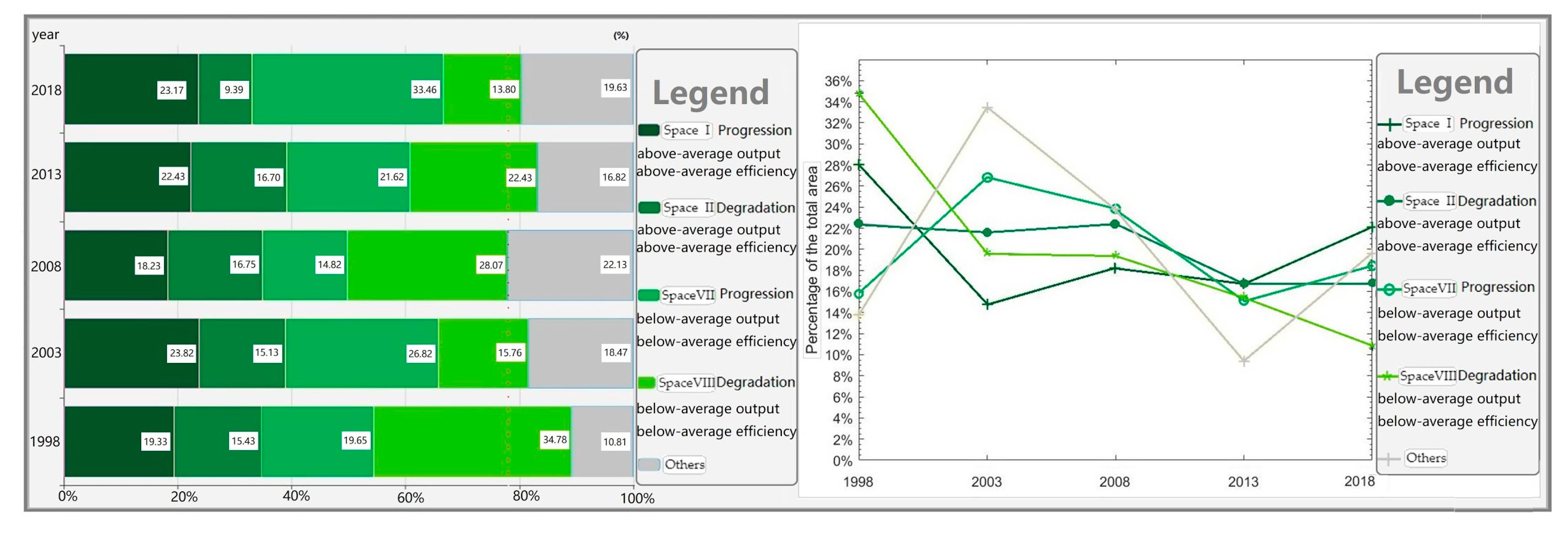
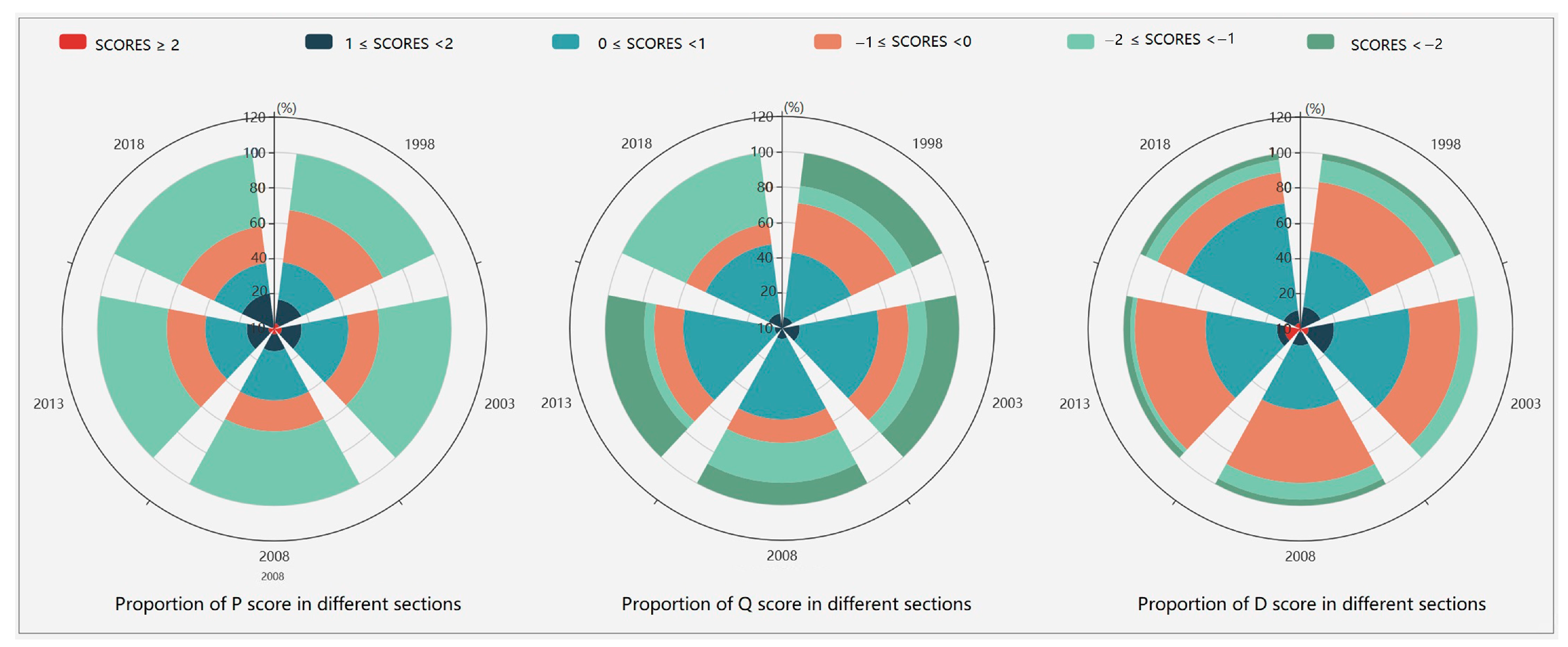
3.1. Multidimensional Assessment Area Results
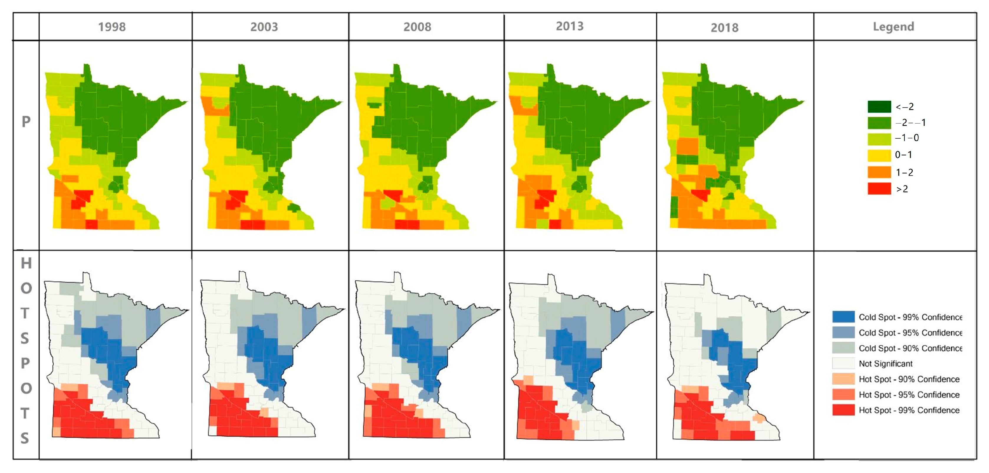
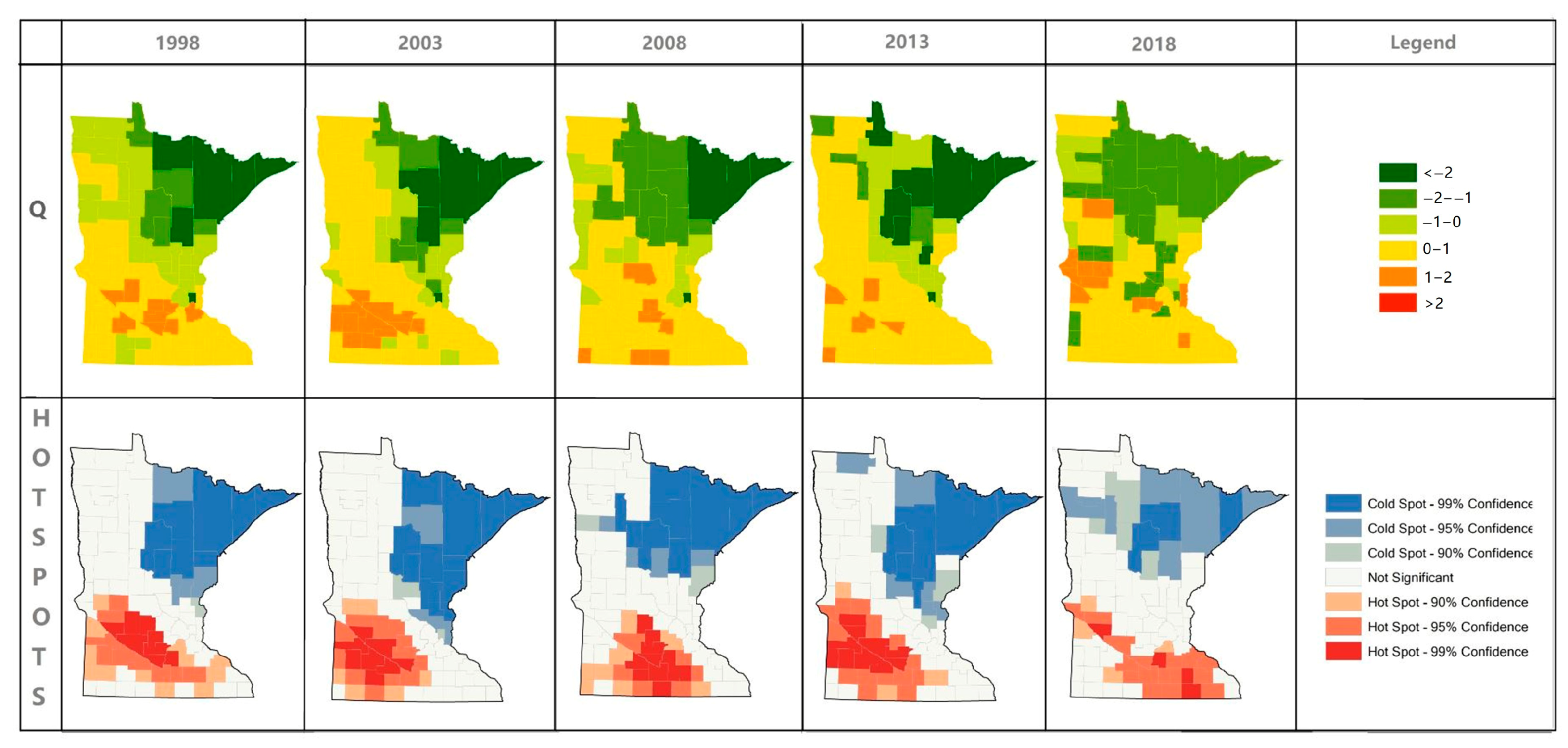
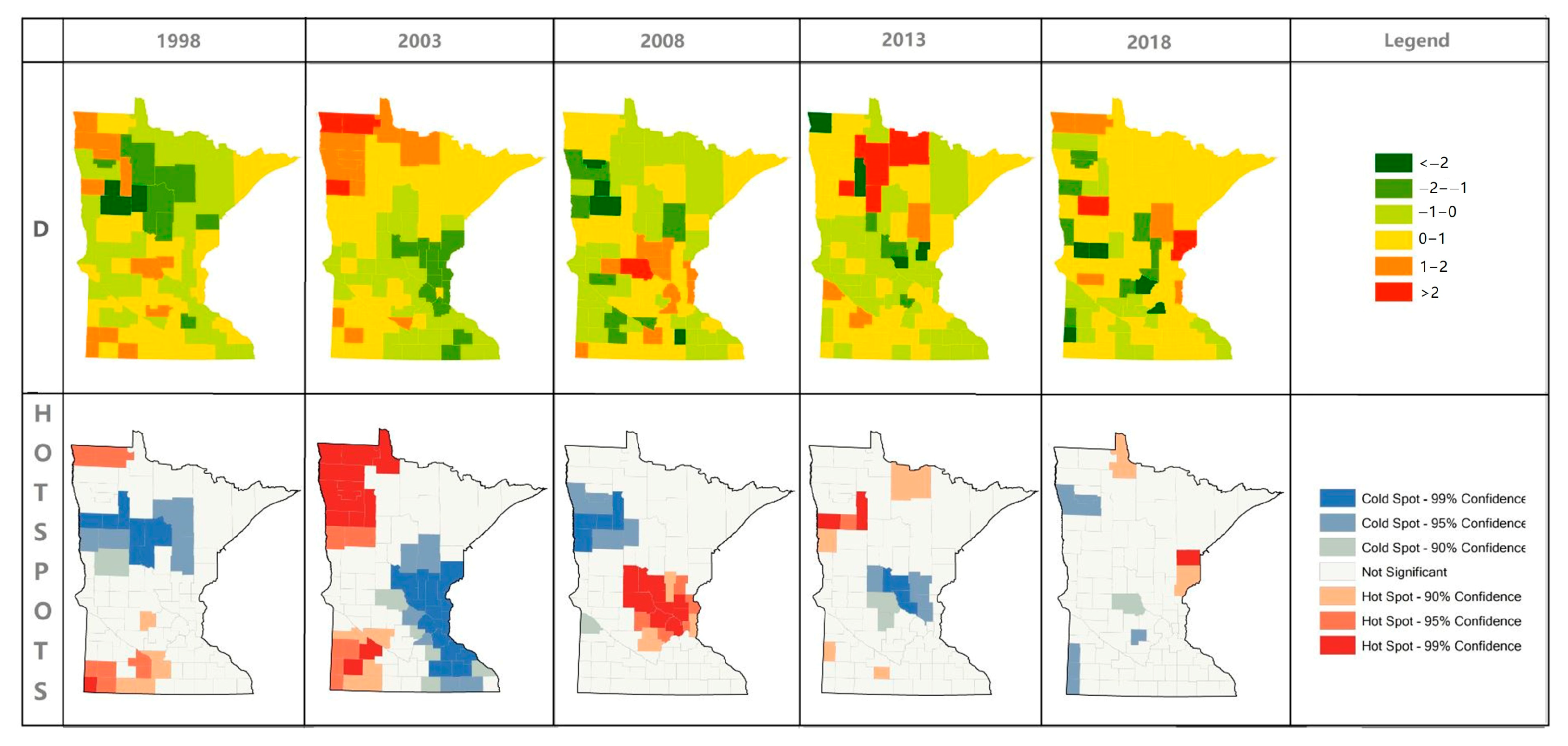
3.2. Multidimensional Assessment Geography Spatial Results
3.2.1. Multidimensional Assessment of Spatial Analysis
3.2.2. Total Output Geospatial Analysis
3.2.3. Efficiency Geospatial Analysis
3.2.4. Trend Geospatial Analysis
3.3. Influencing Factors Analysis
3.3.1. Principal Component Analysis of Influencing Factors
3.3.2. Multiple Linear Regression Analysis of Influencing Factors and Assessment Results
4. Discussion
4.1. Multidimensional Assessment Results Discussion
4.2. Spatiotemporal Patterns of Multidimensional Assessment Results
4.3. Relationship between Multidimensional Assessment Results and Impacting Factors
4.4. Limitations and Future Research Direction
5. Conclusions
Author Contributions
Funding
Conflicts of Interest
References
- Costanza, R.; d’Arge, R.; de Groot, R.; Farber, S.; Grasso, M.; Hannon, B.; Limburg, K.; Naeem, S.; O’Neill, R.V.; Paruelo, J.; et al. The value of the world’s ecosystem services and natural capital. Ecol. Econ. 1998, 25, 3–15. [Google Scholar] [CrossRef]
- Daily, G.C. Nature’s Services; Island Press: Washington, DC, USA, 1997; Volume 3. [Google Scholar]
- Reid, W.V. Millennium Ecosystem Assessment; World Resources Institute: Washington, DC, USA, 2005. [Google Scholar]
- Carpenter, S.R.; Mooney, H.A.; Agard, J.; Capistrano, D.; Defries, R.S.; Díaz, S.; Dietz, T.; Duraiappah, A.K.; Oteng-Yeboah, A.; Pereira, H.M.; et al. Science for managing ecosystem services: Beyond the Millennium Ecosystem Assessment. Proc. Natl. Acad. Sci. USA 2009, 106, 1305–1312. [Google Scholar] [CrossRef] [PubMed]
- Vogt, W. Road to Survival. Soil Sci. 1949, 67, 75. [Google Scholar] [CrossRef]
- Costanza, R.; de Groot, R.; Sutton, P.; van der Ploeg, S.; Anderson, S.J.; Kubiszewski, I.; Farber, S.; Turner, R.K. Changes in the global value of ecosystem services. Glob. Environ. Chang. 2014, 26, 152–158. [Google Scholar] [CrossRef]
- Ratisurakarn, T. Estimating Economic Value of Forest Ecosystem Services: A Meta-Analysis. Ph.D. Thesis, Nida. Available online: https://repository.nida.ac.th/handle/662723737/5073 (accessed on 1 December 2020).
- Davis, H.; Novosad, R. Control, replenishment, and stability of life support systems. J. Spacecr. Rocket. 1964, 1, 96–103. [Google Scholar] [CrossRef]
- Jiang, Y.L.A.Z.G.S. Estimation of Ecosystem Services of Major Forest in China. Acta Phytoecol. Sin. 1999, 23, 426–432. [Google Scholar]
- Bela, G.; Braat, L.; Demeyer, R.; García-Llorente, M. Available online: https://www.researchgate.net/profile/Sander_Jacobs/publication/287444840_Preliminary_guidelines_for_integrated_assessment_and_valuation_of_ecosystem_services_in_specific_policy_contexts/links/59e46b63aca2724cbfe901cf/Preliminary-guidelines-for-integrated-assessment-and-valuation-of-ecosystem-services-in-specific-policy-contexts.pdf (accessed on 17 November 2020).
- Gaodi, X.; Lin, Z.; Chunxia, L.; Yu, X.; Wenhua, L. Applying Value Transfer Method for Eco-Service Valuation in China. jore 2010, 1, 51–59. [Google Scholar]
- Xie, G.; Zhang, C.; Zhang, C.; Xiao, Y.; Lu, C. The value of ecosystem services in China. Resour. Sci. 2015, 37, 1740–1746. [Google Scholar]
- Xie, G.; Zhang, C.; Zhen, L.; Zhang, L. Dynamic changes in the value of China’s ecosystem services. Ecosyst. Serv. 2017, 26, 146–154. [Google Scholar] [CrossRef]
- Farber, S.C.; Costanza, R.; Wilson, M.A. Economic and ecological concepts for valuing ecosystem services. Ecol. Econ. 2002, 41, 375–392. [Google Scholar] [CrossRef]
- Vo, Q.T.; Kuenzer, C.; Vo, Q.M.; Moder, F.; Oppelt, N. Review of valuation methods for mangrove ecosystem services. Ecol. Indic. 2012, 23, 431–446. [Google Scholar] [CrossRef]
- Brander, L. Guidance Manual on Value Transfer Methods for Ecosystem Services; UNEP: Nairobi, Kenya, 2013. [Google Scholar]
- Häyhä, T.; Franzese, P.P. Ecosystem services assessment: A review under an ecological-economic and systems perspective. Ecol. Model. 2014, 289, 124–132. [Google Scholar] [CrossRef]
- Bennett, E.M.; Peterson, G.D.; Gordon, L.J. Understanding relationships among multiple ecosystem services. Ecol. Lett. 2009, 12, 1394–1404. [Google Scholar] [CrossRef]
- Odum, H.T. Environmental Accounting: Energy and Environmental Decision Making; Wiley: Hoboken, NJ, USA, 1996. [Google Scholar]
- Pulselli, F.M.; Coscieme, L.; Bastianoni, S. Ecosystem services as a counterpart of energy flows to ecosystems. Ecol. Model. 2011, 222, 2924–2928. [Google Scholar] [CrossRef]
- Huang, S.-L.; Chen, Y.-H.; Kuo, F.-Y.; Wang, S.-H. Energy-based evaluation of peri-urban ecosystem services. Ecol. Complex. 2011, 8, 38–50. [Google Scholar] [CrossRef]
- Coscieme, L.; Pulselli, F.M.; Marchettini, N.; Sutton, P.C.; Anderson, S.; Sweeney, S. Energy and ecosystem services: A national biogeographical assessment. Ecosyst. Serv. 2014, 7, 152–159. [Google Scholar] [CrossRef]
- Yang, Q.; Liu, G.; Casazza, M.; Hao, Y.; Giannetti, B.F. Energy-based accounting method for aquatic ecosystem services valuation: A case of China. J. Clean. Prod. 2019, 230, 55–68. [Google Scholar] [CrossRef]
- Zhan, J.; Zhang, F.; Chu, X.; Liu, W.; Zhang, Y. Ecosystem services assessment based on energy accounting in Chongming Island, Eastern China. Ecol. Indic. 2019, 105, 464–473. [Google Scholar] [CrossRef]
- Shi, Y.; Shi, D.; Zhou, L.; Fang, R. Identification of ecosystem services supply and demand areas and simulation of ecosystem service flows in Shanghai. Ecol. Indic. 2020, 115, 106418. [Google Scholar] [CrossRef]
- Villa, F.; Ceroni, M.; Bagstad, K.; Johnson, G.; Krivov, S. ARIES (Artificial Intelligence for Ecosystem Services): A new tool for ecosystem services assessment, planning, and valuation. In Proceedings of the 11th Annual BIOECON Conference on Economic Instruments to Enhance the Conservation and Sustainable Use of Biodiversity, Venice, Italy, 1 January 2009; pp. 21–22. [Google Scholar]
- Nelson, E.J.; Daily, G.C. Modelling ecosystem services in terrestrial systems. F1000 Biol. Rep. 2010, 2, 53. [Google Scholar] [CrossRef]
- Bagstad, K.J.; Villa, F.; Johnson, G.W.; Voigt, B. ARIES—Artificial Intelligence for Ecosystem Services: A guide to models and data, version 1.0. ARIES Rep. Ser. 2011, 1, 1–7. [Google Scholar]
- Sánchez-Canales, M.; López Benito, A.; Passuello, A.; Terrado, M.; Ziv, G.; Acuña, V.; Schuhmacher, M.; Elorza, F.J. Sensitivity analysis of ecosystem service valuation in a Mediterranean watershed. Sci. Total Environ. 2012, 440, 140–153. [Google Scholar] [CrossRef] [PubMed]
- Cao, S.; Sanchez-Azofeifa, G.A.; Duran, S.M.; Calvo-Rodriguez, S. Estimation of aboveground net primary productivity in secondary tropical dry forests using the Carnegie–Ames–Stanford approach (CASA) model. Environ. Res. Lett. 2016, 11, 075004. [Google Scholar] [CrossRef]
- Sharps, K.; Masante, D.; Thomas, A.; Jackson, B.; Redhead, J.; May, L.; Prosser, H.; Cosby, B.; Emmett, B.; Jones, L. Comparing strengths and weaknesses of three ecosystem services modelling tools in a diverse UK river catchment. Sci. Total Environ. 2017, 584, 118–130. [Google Scholar] [CrossRef]
- Cong, W.; Sun, X.; Guo, H.; Shan, R. Comparison of the SWAT and InVEST models to determine hydrological ecosystem service spatial patterns, priorities and trade-offs in a complex basin. Ecol. Indic. 2020, 112, 106089. [Google Scholar] [CrossRef]
- Caro, C.; Marques, J.C.; Cunha, P.P.; Teixeira, Z. Ecosystem services as a resilience descriptor in habitat risk assessment using the InVEST model. Ecol. Indic. 2020, 115, 106426. [Google Scholar] [CrossRef]
- Zhang, W.; Yu, Y.; Wu, X.; Pereira, P.; Lucas Borja, M.E. Integrating preferences and social values for ecosystem services in local ecological management: A framework applied in Xiaojiang Basin Yunnan province, China. Land Use Policy 2020, 91, 104339. [Google Scholar] [CrossRef]
- Zhiyun, O.; Rusong, W.; Jingzhu, Z. Ecosystem services and their economic valuation. Chin. J. Appl. Ecol. 1999, 10, 635. [Google Scholar]
- Brauman, K.A.; Daily, G.C.; Ka’eo Duarte, T.; Mooney, H.A. The Nature and Value of Ecosystem Services: An Overview Highlighting Hydrologic Services. Annu. Rev. Environ. Resour. 2007, 32, 67–98. [Google Scholar] [CrossRef]
- Fei, L.; Shuwen, Z.; Jiuchun, Y.; Liping, C.; Haijuan, Y.; Kun, B. Effects of land use change on ecosystem services value in West Jilin since the reform and opening of China. Ecosyst. Serv. 2018, 31, 12–20. [Google Scholar] [CrossRef]
- Rau, A.-L.; von Wehrden, H.; Abson, D.J. Temporal Dynamics of Ecosystem Services. Ecol. Econ. 2018, 151, 122–130. [Google Scholar] [CrossRef]
- Vigerstol, K.L.; Aukema, J.E. A comparison of tools for modeling freshwater ecosystem services. J. Environ. Manag. 2011, 92, 2403–2409. [Google Scholar] [CrossRef] [PubMed]
- Polasky, S.; Nelson, E.; Pennington, D.; Johnson, K.A. The Impact of Land-Use Change on Ecosystem Services, Biodiversity and Returns to Landowners: A Case Study in the State of Minnesota. Environ. Resour. Econ. 2011, 48, 219–242. [Google Scholar] [CrossRef]
- Leh, M.D.K.; Matlock, M.D.; Cummings, E.C.; Nalley, L.L. Quantifying and mapping multiple ecosystem services change in West Africa. Agric. Ecosyst. Environ. 2013, 165, 6–18. [Google Scholar] [CrossRef]
- Wang, Y.; Gao, J.; Wang, J.; Qiu, J. Value assessment of ecosystem services in nature reserves in Ningxia, China: A response to ecological restoration. PLoS ONE 2014, 9, e89174. [Google Scholar] [CrossRef]
- Longato, D.; Gaglio, M.; Boschetti, M.; Gissi, E. Bioenergy and ecosystem services trade-offs and synergies in marginal agricultural lands: A remote-sensing-based assessment method. J. Clean. Prod. 2019, 237, 117672. [Google Scholar] [CrossRef]
- Griffith, J.A. Geographic Techniques and Recent Applications of Remote Sensing to Landscape-Water Quality Studies. Water Air Soil Pollut. Focus 2002, 138, 181–197. [Google Scholar] [CrossRef]
- Doraiswamy, P.C.; Moulin, S.; Cook, P.W.; Stern, A. Crop Yield Assessment from Remote Sensing. Photogramm. Eng. Remote Sens. 2003, 69, 665–674. [Google Scholar] [CrossRef]
- Ferencz, C.; Bognár, P.; Lichtenberger, J.; Hamar, D.; Tarcsai†, G.; Timár, G.; Molnár, G.; Pásztor, S.Z.; Steinbach, P.; Székely, B.; et al. Crop yield estimation by satellite remote sensing. Int. J. Remote Sens. 2004, 25, 4113–4149. [Google Scholar] [CrossRef]
- Prasad, A.K.; Chai, L.; Singh, R.P.; Kafatos, M. Crop yield estimation model for Iowa using remote sensing and surface parameters. Int. J. Appl. Earth Obs. Geoinf. 2006, 8, 26–33. [Google Scholar] [CrossRef]
- Feld, C.K.; Martins da Silva, P.; Paulo Sousa, J.; de Bello, F.; Bugter, R.; Grandin, U.; Hering, D.; Lavorel, S.; Mountford, O.; Pardo, I.; et al. Indicators of biodiversity and ecosystem services: A synthesis across ecosystems and spatial scales. Oikos 2009, 118, 1862–1871. [Google Scholar] [CrossRef]
- Markogianni, V.; Dimitriou, E.; Karaouzas, I. Water quality monitoring and assessment of an urban Mediterranean lake facilitated by remote sensing applications. Environ. Monit. Assess. 2014, 186, 5009–5026. [Google Scholar] [CrossRef] [PubMed]
- De Araujo Barbosa, C.C.; Atkinson, P.M.; Dearing, J.A. Remote sensing of ecosystem services: A systematic review. Ecol. Indic. 2015, 52, 430–443. [Google Scholar] [CrossRef]
- Harwood, T.D.; Donohue, R.J.; Williams, K.J.; Ferrier, S.; McVicar, T.R.; Newell, G.; White, M. Habitat Condition Assessment System: A new way to assess the condition of natural habitats for terrestrial biodiversity across whole regions using remote sensing data. Methods Ecol. Evol. 2016, 7, 1050–1059. [Google Scholar] [CrossRef]
- Vargas, L.; Willemen, L.; Hein, L. Assessing the Capacity of Ecosystems to Supply Ecosystem Services Using Remote Sensing and an Ecosystem Accounting Approach. Environ. Manag. 2019, 63, 1–15. [Google Scholar] [CrossRef]
- Wikipedia Contributors Minnesota. Available online: https://en.wikipedia.org/w/index.php?title=Minnesota&oldid=985368473 (accessed on 27 October 2020).
- Agriculture. Available online: https://www.dli.mn.gov/business/workforce/agriculture (accessed on 27 October 2020).
- USDA/NASS QuickStats Ad-Hoc Query Tool. Available online: https://quickstats.nass.usda.gov/ (accessed on 20 November 2020).
- USGS Landsat 8 Collection 1 Tier 1 TOA Reflectance. Available online: https://developers.google.com/earth-engine/datasets/catalog/LANDSAT_LC08_C01_T1_TOA (accessed on 20 November 2020).
- MOD11A2.006 Terra Land Surface Temperature and Emissivity 8-Day Global 1 km. Available online: https://developers.google.com/earth-engine/datasets/catalog/MODIS_006_MOD11A2 (accessed on 20 November 2020).
- Daymet V3: Daily Surface Weather and Climatological Summaries. Available online: https://developers.google.com/earth-engine/datasets/catalog/NASA_ORNL_DAYMET_V3 (accessed on 20 November 2020).
- USDA/NASS 2019 State Agriculture Overview for Minnesota. Available online: https://www.nass.usda.gov/Quick_Stats/Ag_Overview/stateOverview.php?state=MINNESOTA (accessed on 20 November 2020).
- Fageria, N.K.; Baligar, V.C.; Clark, R.B. Micronutrients in Crop Production. In Advances in Agronomy; Sparks, D.L., Ed.; Academic Press: Cambridge, MA, USA, 2002; Volume 77, pp. 185–268. [Google Scholar]
- Tukey, J.W. Exploratory Data Analysis; Pearson: Reading, MA, USA, 1977; Volume 2. [Google Scholar]
- Aghajani, M.A.; Dezfoulian, R.S.; Arjroody, A.R.; Rezaei, M. Applying GIS to Identify the Spatial and Temporal Patterns of Road Accidents Using Spatial Statistics (case study: Ilam Province, Iran). Transp. Res. Procedia 2017, 25, 2126–2138. [Google Scholar] [CrossRef]
- Almanac, O.F. Planting Calendar for Minneapolis, MN. Available online: https://www.almanac.com/gardening/planting-calendar/mn/Minneapolis (accessed on 26 November 2020).
- Peltonen-Sainio, P.; Jauhiainen, L.; Hakala, K.; Ojanen, H. Climate change and prolongation of growing season: Changes in regional potential for field crop production in Finland. Agric. Food Sci. 2009, 18, 171–190. [Google Scholar] [CrossRef]
- Johnson, G.A.; Kantar, M.B.; Betts, K.J.; Wyse, D.L. Field Pennycress Production and Weed Control in a Double Crop System with Soybean in Minnesota. Agron. J. 2015, 107, 532–540. [Google Scholar] [CrossRef]
- Semmens, K.A.; Anderson, M.C.; Kustas, W.P.; Gao, F.; Alfieri, J.G.; McKee, L.; Prueger, J.H.; Hain, C.R.; Cammalleri, C.; Yang, Y.; et al. Monitoring daily evapotranspiration over two California vineyards using Landsat 8 in a multi-sensor data fusion approach. Remote Sens. Environ. 2016, 185, 155–170. [Google Scholar] [CrossRef]
- Pearson, K. Principal components analysis. Lond. Edinb. Dublin Philos. Mag. J. Sci. 1901, 6, 559. [Google Scholar] [CrossRef]
- Wikipedia Contributors Principal Component Analysis. Available online: https://en.wikipedia.org/w/index.php?title=Principal_component_analysis&oldid=979916858 (accessed on 6 October 2020).
- Goodwin, B.K.; Vado, L.A. Public Responses to Agricultural Disasters: Rethinking the Role of Government. Can. J. Agric. Econ. 2007, 55, 399–417. [Google Scholar] [CrossRef]
- Nadolnyak, D.; Hartarska, V. Agricultural disaster payments in the southeastern US: Do weather and climate variability matter? Null 2012, 44, 4331–4342. [Google Scholar] [CrossRef]
- Database, E.F.S. EWG’s Farm Subsidy Database. Available online: https://farm.ewg.org/progdetail.php?fips=27000&progcode=total_dis®ionname=Minnesota (accessed on 2 November 2020).
- Smith, V.H.; Goodwin, B.K. The Environmental Consequences of Subsidized Risk Management and Disaster Assistance Programs. Annu. Rev. Resour. Econ. 2013, 5, 35–60. [Google Scholar] [CrossRef]
- Modernel, P.; Rossing, W.A.H.; Corbeels, M. Land use change and ecosystem service provision in Pampas and Campos grasslands of southern South America. Environmentalist 2016, 11, 113002. [Google Scholar] [CrossRef]
- Song, W.; Deng, X. Land-use/land-cover change and ecosystem service provision in China. Sci. Total Environ. 2017, 576, 705–719. [Google Scholar] [CrossRef]
- Alemu, W.G.; Henebry, G.M.; Melesse, A.M. Land Surface Phenologies and Seasonalities in the US Prairie Pothole Region Coupling AMSR Passive Microwave Data with the USDA Cropland Data Layer. Remote Sens. 2019, 11, 2550. [Google Scholar] [CrossRef]
- Sun, X.; Tang, H.; Yang, P.; Hu, G.; Liu, Z.; Wu, J. Spatiotemporal patterns and drivers of ecosystem service supply and demand across the conterminous United States: A multiscale analysis. Sci. Total Environ. 2020, 703, 135005. [Google Scholar] [CrossRef]
- Minnesota Population 2020 (Demographics, Maps, Graphs). Available online: https://worldpopulationreview.com/states/minnesota-population (accessed on 1 October 2020).
- Bolton, D.K.; Friedl, M.A. Forecasting crop yield using remotely sensed vegetation indices and crop phenology metrics. Agric. For. Meteorol. 2013, 173, 74–84. [Google Scholar] [CrossRef]
- Kern, A.; Barcza, Z.; Marjanović, H.; Árendás, T.; Fodor, N.; Bónis, P.; Bognár, P.; Lichtenberger, J. Statistical modelling of crop yield in Central Europe using climate data and remote sensing vegetation indices. Agric. For. Meteorol. 2018, 260, 300–320. [Google Scholar] [CrossRef]
- Willcock, S.; Martínez-López, J.; Hooftman, D.A.P.; Bagstad, K.J.; Balbi, S.; Marzo, A.; Prato, C.; Sciandrello, S.; Signorello, G.; Voigt, B.; et al. Machine learning for ecosystem services. Ecosyst. Serv. 2018, 33, 165–174. [Google Scholar] [CrossRef]
- Wan, Z.; Gong, M.; Jiang, F. An Estimation Framework for Economic Cost of Land Use Based on Artificial Neural Networks and Principal Component Analysis with R. In Proceedings of the 2019 IEEE 3rd Advanced Information Management, Communicates, Electronic and Automation Control Conference (IMCEC), Chongqing, China, 1–13 October 2019; pp. 204–209. [Google Scholar]
- Peponi, A.; Morgado, P.; Trindade, J. Combining Artificial Neural Networks and GIS Fundamentals for Coastal Erosion Prediction Modeling. Sustain. Sci. Pract. Policy 2019, 11, 975. [Google Scholar] [CrossRef]
- Mirghaderi, S.-H. Using an artificial neural network for estimating sustainable development goals index. Manag. Environ. Qual. Int. J. 2020, 31, 1023–1037. [Google Scholar] [CrossRef]
- Liang, B.; Liu, H.; Quine, T.A.; Chen, X.; Hallett, P.D.; Cressey, E.L.; Zhu, X.; Cao, J.; Yang, S.; Wu, L.; et al. Analysing and simulating spatial patterns of crop yield in Guizhou Province based on artificial neural networks. Prog. Phys. Geogr. Earth Environ. 2020, 16, 0309133320956631. [Google Scholar] [CrossRef]


| Space | P | Q | D | Properties | Description |
|---|---|---|---|---|---|
| I | + | + | + | The total output, efficiency, and trend index are above average. | Progression |
| II | + | + | − | The total output and efficiency are above average, but the trend index is below average. | Degradation |
| III | + | − | + | Although the efficiency is below average, it has been raised. The above-average output depends on the larger ecosystem area. | Progression |
| IV | + | − | − | The efficiency is below average and it has degraded. The above-average output depends on ecosystem scales. | Degradation |
| V | − | + | + | The output is below average, indicating that the ecosystem scale should be expanded. | Progression |
| VI | − | + | − | Both the output and the trend index are below average, but it has high efficiency. | Degradation |
| VII | − | − | + | The output and efficiency are below average, but it has an above-average trend index. | Progression |
| VIII | − | − | − | All three indices are below average. It has a lower output and efficiency. Simultaneously and unfortunately, it has degraded. | Degradation |
| Index | Formulation | Introduction | |
|---|---|---|---|
| P | is P-score of county i in the year j, is the crop production of county i in the year j, is the average crop production of the state in year j, is the crop production standard variance of all counties in year j. | ||
| Q | is the Q-score of ecosystem service efficiency of county i in the year j, is the yield of county i in the year j, is the average crop yield of the state in year j, is the yield standard variance of all counties in year j. | ||
| D | is the D-score of the county i in the year j, is the annual efficiency change in county i in year j, is the average of annual efficiency change in the entire state in year j, is the annual efficiency change standard variance of all counties in year j. |
| Z Score (Standard Deviation) | p Value (Probability) | Confidence Level |
|---|---|---|
| z < −1.65 or z > +1.65 | p < 0.1 | 90% |
| z < −1.95 or z > +1.95 | p < 0.05 | 95% |
| z < −2.58 or z > +2.58 | p < 0.01 | 99% |
| Agricultural District | Counties |
|---|---|
| Central | Scott, Wadena, Sherburne, Morrison, Renville, Todd, Meeker, McLeod, Wright, Benton, Sibley, Carver, Stearns, Kandiyohi |
| East Central | Aitkin, Hennepin, Ramsey, Crow Wing, Carlton, Washington, Pine, Isanti, Anoka, Mille Lacs, Chisago, Kanabec |
| North Central | Koochiching, Cass, Lake of the Woods, Hubbard, Itasca, Beltrami |
| Northeast | Cook, Lake, St. Louis |
| Northwest | Becker, Clay, Marshall, Red Lake, Norman, Roseau, Mahnomen, Polk, Pennington, Kittson, Clearwater |
| South Central | Faribault, Martin, Rice, Blue Earth, Waseca, Watonwan, Brown, Le Sueur, Freeborn, Nicollet, Steele |
| Southeast | Dodge, Winona, Mower, Wabasha, Goodhue, Houston, Dakota, Fillmore, Olmsted |
| Southwest | Cottonwood, Redwood, Murray, Rock, Lyon, Jackson, Nobles, Lincoln, Pipestone |
| West Central | Wilkin, Traverse, Yellow Medicine, Grant, Chippewa, Swift, Otter Tail, Stevens, Lac qui Parle, Big Stone, Douglas, Pope |
| Variables | Principal Component | ||
|---|---|---|---|
| PDI | 0.5644 | 0.1860 | −0.0430 |
| NDVI | 0.1870 | 0.5365 | 0.7947 |
| RF | 0.5970 | −0.0340 | −0.2448 |
| DT | 0.5375 | −0.3896 | 0.0750 |
| DIF | 0.0337 | 0.7243 | −0.5487 |
| Objects | Score | Critical Value | Results | |
|---|---|---|---|---|
| P | 0.005 | 23.46 | 3.76 | credible |
| Q | 0.005 | 14.19 | 3.76 | credible |
| 0.1 | 2.91 | 1.92 | credible | |
| 0.1 | 3.25 | 1.92 | credible |
Publisher’s Note: MDPI stays neutral with regard to jurisdictional claims in published maps and institutional affiliations. |
© 2020 by the authors. Licensee MDPI, Basel, Switzerland. This article is an open access article distributed under the terms and conditions of the Creative Commons Attribution (CC BY) license (http://creativecommons.org/licenses/by/4.0/).
Share and Cite
Shi, D.; Shi, Y.; Wu, Q.; Fang, R. Multidimensional Assessment of Food Provisioning Ecosystem Services Using Remote Sensing and Agricultural Statistics. Remote Sens. 2020, 12, 3955. https://doi.org/10.3390/rs12233955
Shi D, Shi Y, Wu Q, Fang R. Multidimensional Assessment of Food Provisioning Ecosystem Services Using Remote Sensing and Agricultural Statistics. Remote Sensing. 2020; 12(23):3955. https://doi.org/10.3390/rs12233955
Chicago/Turabian StyleShi, Donghui, Yishao Shi, Qiusheng Wu, and Ruibo Fang. 2020. "Multidimensional Assessment of Food Provisioning Ecosystem Services Using Remote Sensing and Agricultural Statistics" Remote Sensing 12, no. 23: 3955. https://doi.org/10.3390/rs12233955
APA StyleShi, D., Shi, Y., Wu, Q., & Fang, R. (2020). Multidimensional Assessment of Food Provisioning Ecosystem Services Using Remote Sensing and Agricultural Statistics. Remote Sensing, 12(23), 3955. https://doi.org/10.3390/rs12233955