Article

Monitoring the Recovery after 2016 Hurricane Matthew in Haiti via Markovian Multitemporal Region-Based Modeling

1
Department of Electrical, Electronic and Telecommunication Engineering and Naval Architecture (DITEN), University of Genoa, Via all’Opera Pia 11a, I-16145 Genoa, Italy
2
Italian Space Agency (ASI), Via del Politecnico, I-00133 Rome, Italy
3
Department of Civil, Chemical, and Environmental Engineering (DICCA), University of Genoa, Via Montallegro 1, I-16145 Genoa, Italy
4
CIMA Foundation, Via Magliotto 1, I-17100 Savona, Italy
*
Author to whom correspondence should be addressed.
Remote Sens. 2021, 13(17), 3509; https://doi.org/10.3390/rs13173509
Submission received: 30 June 2021 / Revised: 27 August 2021 / Accepted: 30 August 2021 / Published: 4 September 2021

Abstract

:
The aim of this paper is to address the monitoring of the recovery phase in the aftermath of Hurricane Matthew (28 September–10 October 2016) in the town of Jérémie, southwestern Haiti. This is accomplished via a novel change detection method that has been formulated, in a data fusion perspective, in terms of multitemporal supervised classification. The availability of very high resolution images provided by last-generation satellite synthetic aperture radar (SAR) and optical sensors makes this analysis promising from an application perspective and simultaneously challenging from a processing viewpoint. Indeed, pursuing such a goal requires the development of novel methodologies able to exploit the large amount of detailed information provided by this type of data. To take advantage of the temporal and spatial information associated with such images, the proposed method integrates multisensor, multisource, and contextual information. Markov random field modeling is adopted here to integrate the spatial context and the temporal correlation associated with images acquired at different dates. Moreover, the adoption of a region-based approach allows for the characterization of the geometrical structures in the images through multiple segmentation maps at different scales and times. The performances of the proposed approach are evaluated on multisensor pairs of COSMO-SkyMed SAR and Pléiades optical images acquired over Jérémie, in the aftermath of and during the three years after Hurricane Matthew. The effectiveness of the change detection results is analyzed both quantitatively, through the computation of accuracy measures on a test set, and qualitatively, by visual inspection of the classification maps. The robustness of the proposed method with respect to different algorithmic choices is also assessed, and the detected changes are discussed in relation to the recovery endeavors in the area and ground-truth data collected in the field in April 2019.

1. Introduction

In the last decades, advances in the design and development of optical and synthetic aperture radar (SAR) satellite sensors have favored the deployment of new technological solutions able to acquire imagery at very high spatial resolution (VHR) with short revisit time. Moreover, the combined use of such systems commonly leads to analysis of data characterized by different acquisition modes and geometries and different spatial and temporal resolutions. In this context, the possibility of using pattern recognition and image processing techniques for the automatic processing of such a variety of remote sensing data represents an effective approach to tackle applications such as environmental monitoring, environmental disaster management, and disaster prevention tasks. Indeed, being able to take advantage of heterogeneous data (for example, by jointly processing pairs of images taken at different times and possibly by different sensors and at different resolutions, independently of the acquisition characteristics) to highlight the temporal evolution of the Earth surface is of paramount importance in this field of application. The main opportunity is to take advantage of the complementarity of such information sources to map effectively the different types of change that may occur between two different moments in time, in either a short-term or a long-term scenario.
The study presented in this paper falls within this framework and was conducted in the context of the Committee on Earth Observation Satellites—Disaster Risk Management (CEOS-DRM) project led and funded by the Italian Space Agency (ASI), in collaboration with the International Center for Environmental Monitoring (CIMA) Foundation and the University of Genoa. The paper proposes an automatic change detection method that is aimed at supporting the monitoring of the recovery phase in the aftermath of particularly disruptive events. Specifically, Hurricane Matthew (28 September–10 October 2016), the most powerful storm of the 2016 Atlantic hurricane season, was chosen as a case study to demonstrate the potential of the developed tool. This natural disaster struck the southwest departments of Haiti in early October 2016 as a category 4 hurricane. The combined effects of wind, coastal flooding, and rain caused major inundations, landslides, and the destruction of many urban infrastructures, agricultural crops, and natural ecosystems. Overall, the hurricane led to more than 500 lives lost, 128 people missing, 439 injured, and 2.1 million people affected, including 895,000 children [1].
Recovery from such a major disaster is a process that leads to changes in land use, reconstruction of the built environment, and other types of land cover transitions that are likely to occur in the affected areas both near- and long-term, i.e., immediately and from one to three years after the event [2]. Determining how to capture, document, and monitor such changes by exploiting multisensor satellite data is the overall application framework within which the present research has been developed.
The proposed change detection problem is formulated from a data fusion perspective [3,4] via Markovian modeling [5,6,7] by generalizing the technique presented in [8]. The change detection problem is addressed via a joint multitemporal classification based on multisensor imagery composed of optical and SAR acquisitions. In detail, it combines the Markov random field (MRF) theory with a region-based approach and with ensemble and kernel learning concepts. The method is general in its applicability to arbitrary optical and SAR data. However, consistently with the objectives of the above-described application, the experimental analysis reported in this paper is focused on the case of COSMO-SkyMed and Pléiades images, in a data fusion perspective.
In particular, change detection is addressed through a multitemporal supervised classification approach. Classification maps at two different dates are jointly computed by taking into consideration the multitemporal dataset. The change map is intrinsically generated within such a supervised procedure. This choice is related to both the specific recovery application and the employed VHR satellite data, as it favors the explicit identification of land cover classes and transitions within the change detection product. Indeed, the monitoring of the recovery phase in the aftermath of a disaster calls for a detailed understanding of the observed data and for the characterization of the typology of the changes that occurred.
MRFs represent a general family of probabilistic models for two-dimensional stochastic processes that are defined over a discrete pixel lattice. They allow multisource data and contextual information to be included in Bayesian image analysis tasks. They provide for the spatial modeling and data fusion capabilities [5] that are necessary here to compute the classification maps and the change map integrating all the multitemporal and multisensor input data. Computationally, through MRF modeling, the Hammersley–Clifford theorem [5] allows formulating the maximum a posteriori (MAP) decision rule in terms of the minimization of a suitable energy function.
The energy function [5,6,9] of the proposed Markovian fusion framework comprises different contributions related to (i) the spatial relationships between neighboring pixels of the imaged scene, (ii) the temporal relationships between the same location at different acquisition times, and (iii) the multiscale information conveyed by a region-based analysis of the input imagery. Concerning the spatial and temporal relationships, an ad hoc graph is constructed on top of the multitemporal input data. Such a graph is used, within the Markovian framework, to integrate prior information in the fusion process. The resulting change map is then characterized by spatial and temporal regularization that ensures consistency between the classification maps, and thus in the change detection product. This allows taking into account both spatial and temporal information in the monitoring of the recovery process across each pair of considered observation times.
Concerning multiscale information, the VHR nature of the input image requires characterization of both large geometrical structures and smaller spatial details. This is accomplished here by exploiting both fine and coarse scales thanks to the use of multiple segmentation maps. Indeed, the third component of the developed Markov model is related to the results of a segmentation method applied with the goal of extracting details at different scales. The opportunity of using region-based concepts is consistent with the broad framework of geospatial object-based image analysis (OBIA) [10]. In the context of remote sensing image classification, the use of data at different resolutions provides at the same time benefits and drawbacks depending on the final goal of the classification task. Indeed, on one hand, high-resolution images allow for the detection of the spatial–geometrical configuration and the generation of land cover maps with detailed thematic classes. On the other hand, the high spatial heterogeneity conveyed by high-resolution observations may not lead to the identification of the main thematic classes, such as urban or built-up land covers. The use of segmentation maps at different scales as an input of the classification process makes it possible to take advantage of both fine-scale and coarse-scale data representations.
It is worth mentioning that a first preliminary formulation of the work presented in this paper has been published as a conference paper [11]. The goal of that publication was to give a preliminary idea of the method and briefly show the first results. In the present article, we extend the conference paper in terms of both a more detailed methodological description and of an expanded experimental analysis over a longer timeframe after the hurricane. Furthermore, validation of the classification maps is made by means of ground-truth data collected in the field in April 2019. The outcomes are discussed in relation to land management and anthropogenic processes occurring in Jérémie.
The paper is organized as follows: Section 2 summarizes the state-of-the-art methods for the identification of land cover changes and transitions from remote sensing imagery. Then, Section 3 describes materials and methods, presenting the case study and the available dataset (Section 3.1) and the proposed methodological approach (Section 3.2, Section 3.3 and Section 3.4). Section 4 presents the results achieved by the developed method with details on the produced change maps and confusion matrices for a quantitative evaluation of the performances. Section 5 provides the discussion of the results with respect to the problem at hand, i.e., the monitoring of the recovery phase in the aftermath of Hurricane Matthew. Finally, Section 6 summarizes the main conclusions.

2. Previous Work on Land Cover Change Detection

In the last 30 years, the increased availability of satellite data with shorter revisit period and finer spatial resolution, together with the related time series of images acquired on a regular basis, have attracted the attention of the remote sensing community. In the literature, several methodological approaches have been developed in the context of multitemporal remote sensing analysis to characterize the changes in land cover [12,13,14,15]. Various review papers adopt different categorization principles to classify these change detection approaches into separate categories.
A first scheme was presented in [12] and uses a categorization based on the order by which the input images are processed. In [16,17], classification maps are produced independently for each acquisition date, and then a comparative study of the obtained classification maps is performed to highlight the changes that occurred. On the contrary, similarly to the work proposed in this paper, in [18,19,20], different images are analyzed simultaneously by taking into account their multitemporal relationships from the beginning. A second classification scheme, proposed in [21], focuses the attention on the object of analysis, distinguishing between classification approaches [19,22] and change measurements [23,24]. Moreover, a different scheme is proposed in [25] and identifies three categories depending on the role of the time dimension. Finally, the review in [3] discriminates between methods performing the fusion of the multitemporal data at the feature level or at the decision level. In the former case, multitemporal information is extracted through the generation of new features able to emphasize changes in the dataset. Conversely, in the latter case, higher-level analysis is conducted by applying suitable decision rules to identify land cover classes and highlight the changes.
Concerning the multitemporal fusion at the feature level, a first type of approach is represented by techniques based on image comparison. Such techniques are usually sensor-specific and are designed by considering the noise model for the data at hand. The image ratioing approach, sometimes expressed on the logarithmic scale, is a common example [26,27] in the case of SAR data affected by the multiplicative speckle component. Conversely, techniques such as the univariate image differencing [28,29] or the change vector analysis (CVA) [30,31] are usually applied in the case of data collected by passive optical sensors, whose noise is usually modeled as additive Gaussian. Other relevant families of approaches are the transformation techniques (e.g., the principal component analysis (PCA) [32]); the regression approaches [33]; the methods based on distance functions and similarity measures (e.g., the Kullback–Leibler divergence [34]); and additional methods based, for instance, on statistical mixture models, backscattering coefficient, H-α decompositions, and polarimetric signatures.
Another alternative solution is represented by the formalization of the change detection problem in an unsupervised Bayesian framework. In this context, a predefined statistical distribution for the classes associated with changed and unchanged pixels, according to the specific type of data, is assumed. After the application of implicit or explicit automatic parameter estimation processes, the change detection task is performed through pattern recognition approaches [31,35].
This discussion points out that multitemporal fusion at the feature level is mainly related to unsupervised detection approaches whose final product is often limited to the identification of changed and unchanged areas; i.e., it is usually a binary output map. These approaches are especially appealing for the application in emergency scenarios where the main goal is to identify changed areas accurately and with short computation times or in event-based risk assessment through data mining in long image archives (e.g., [36,37]).
Concerning the methods belonging to the category of multitemporal fusion at the decision level, they are explicitly designed to identify land cover classes and land cover transitions, providing a better understanding of the observed data and characterizing the typology of the changes that occurred. Most of the approaches in this category involve supervised and semisupervised classification techniques, which require the availability of a labeled training set. In contrast to the methods described above, this is consistent with the application to a detailed monitoring study, but it would poorly match the requirements of the application to an emergency. These techniques allow simultaneously performing change detection and change classification on multitemporal time series of images. Three different subgroups can be identified: (i) postclassification comparison (PCC), (ii) direct multidate classification, and (iii) joint multitemporal classification.
PCC methods accomplish the change detection task by classifying separately each image of the multitemporal dataset and performing a comparison between the obtained thematic maps. On one hand, this allows minimizing the impacts of the sensor and atmospheric differences resulting from the asynchronous acquisition of the images in time series. On the other hand, the simple formulation of PCC methods is not able to consider the temporal correlation. Thus, the overall performances are strictly connected to the results generated on each image by the adopted classifier. In the literature, there exist examples of PCC methods using pixel-by-pixel classification [38,39] and region-based approaches [40,41].
In order to take into account temporal correlations, direct multidate and joint multitemporal methods carry out a single analysis on a combined dataset containing two or more images acquired on different dates. In the case of direct multidate classification, the feature vector associated with each image pixel is composed of the feature values of all the images stacked together. Assuming that training pixels related to the same area on the ground are available at different dates, a classifier is trained separately for the identification of each land-cover transition [42]. An intrinsic limitation of such approaches is that they do not model the temporal structure of the data. Indeed, the joint statistics of the features on either date and the joint statistics across the observation dates are substantially merged, without attempting to model their different semantics. Conversely, joint multitemporal classification allows the integration of a dataset of two or more dates into a single analysis process. In a Bayesian framework, two different strategies can be adopted in order to tackle this task: the cascade approach and the mutual approach. In the former case, each image is classified on the basis of itself and of previous images by removing the coupling between the spectral and temporal dimensions [43]. On the contrary, the latter classifies each image on the basis of the previous and the subsequent images of the dataset [22]. From an application-oriented viewpoint, the cascade approach is typical of situations in which a pre-existing land cover map should be updated according to newly available satellite imagery. The mutual approach meets the requirements of the applications in which a full time series of images, all collected in the past, should be used to study the related temporal phenomena.
The above analysis recalls how classification methods have proven effective in the application to land cover change detection. The main reason lies in their capability to intrinsically exploit multitemporal and possibly multisensor, multiscale, and multiresolution information. Indeed, they make it possible to produce land cover transition maps by taking advantage of the large amount of information related to images acquired on the same ground area on different dates and by sensors of different types (e.g., optical multispectral and SAR images). Nevertheless, the integration of such a large amount of data in the case of last-generation VHR imagery may represent a challenge. On one hand, VHR images are characterized by strong correlation between neighboring pixels. On the other hand, the spatial behavior of the pixel intensity is heterogeneous and allows distinguishing among spectral responses produced by different ground objects and materials. Four main methodological approaches exist that are able to incorporate spatial contextual information in image analysis: (i) spatial feature extraction, (ii) region-based or object-based methods, (iii) probabilistic graphical models, and (iv) deep learning methods based on convolutional neural networks (CNNs).
The first approach relies on the inclusion in the classification process of further features able to capture the spatial relationship among the intensities of neighboring pixels. Classical examples include Haralick’s features and the grey level co-occurrence matrix [44], mathematical morphology [45], and wavelet transforms [46].
Concerning the second family of approaches, in the classification process, region-based and object-based methods usually include the results obtained by the application of a segmentation algorithm able to capture the geometrical structure associated with the image. Examples include region-growing algorithms [47], fuzzy-connectedness techniques [48], watershed methods [49], and hierarchical algorithms [50]. The use of a region-based approach allows dealing with data at very high resolution. Indeed, the use of segmentation maps at different scales as an input of the classification process makes it possible to take advantage of both high-resolution and coarse-resolution observations.
The third approach represents not only an additional methodology for the integration of spatial contextual information, but also a powerful general data fusion framework, which can play an important role in the change detection task as well. Probabilistic graphical models are a general family of models for the dependence across a collection of random variables. They are formalized in terms of a probabilistic formulation on top of a graph topology, typically associated with Markovianity properties. In the application to remote sensing image processing, MRF and conditional random field (CRF) models on undirected graphs are especially prominent [51,52,53,54]. Differently from MRFs, which are designed to model the prior distribution of the desired output map, CRFs [55] have been introduced to formalize the Markovianity property with regard to the posterior distribution directly, often further enhancing modeling flexibility. The remarkable results obtained by this Markovian approach to multisource fusion in the remote sensing field can be seen in various examples involving multisensor [56], multitemporal [22], multiresolution [57], or multichannel imagery [58], or combinations of the above [59,60].
On one hand, in the case of methods based on spatial features, one often speaks of “feature engineering” to emphasize that the rationale of the feature extraction stage is determined by the specific interpretation of the feature semantic, as meant and defined by a human operator. On the other hand, effective approaches have been recently developed using deep learning concepts [61]. In particular, architectures based on CNNs intrinsically extract spatial contextual features through convolutional filtering and pooling operators. These features are meant to provide data representations at progressively more abstract semantic levels and are determined by the learning of the network based on the training set and not engineered by the operator. An operational limitation is generally due to the need for large annotated ground truth to be used for training purposes. Examples of state-of-the-art solutions based on CNNs are [62,63,64,65].

3. Materials and Methods

3.1. Case Study

The proposed method to address land cover change was tested in support of the monitoring of the recovery phase after Hurricane Matthew, which struck Haiti on 4 October 2016. To this end, the study area encompassed the coastal zone around the town of Jérémie, capital of the Grande Anse department in the southwest of Haiti, i.e., the main urban settlement that was dramatically affected by the hurricane. Jérémie was selected among the priority areas of interest by the Haitian authorities, the technical institutions, and the space agencies involved in the CEOS Haiti Recovery Observatory (RO) project [2]. The Haiti RO was a 4-year-long initiative carried out in the framework of the CEOS Working Group on Disasters (WGDisasters), chaired by the Italian Space Agency (ASI) during the development of the present work, and coordinated by the French National Centre for Space Studies (CNES) and the National Geospatial Information Center (CNIGS) of Haiti. Among its goals, the project aimed to demonstrate in a high-profile context the value of using satellite Earth observation to support recovery from a major disaster, in the near term (e.g., support for postdisaster needs assessment (PDNA) process [66]) and long term (e.g., major recovery planning and monitoring, estimated to be from 1 to 3 years) [2]. In this framework, the CEOS-DRM project, which is the baseline for the work that is proposed in this paper, contributed to the generation of the thematic product “watershed/flood” of the Haiti RO product portfolio [1].
Following the Recovery Observatory Operations Plan [2], CNES and ASI activated dedicated satellite data acquisition campaigns with the Pléiades and COSMO-SkyMed constellations, respectively, the latter in addition to a regional-scale coverage with TerraSAR-X by the German Aerospace Center (DLR) and Sentinel-1 by the European Space Agency (ESA) [67]. It is in this framework that the present study exploited the bespoke dataset of VHR optical (Pléiades) and SAR (COSMO-SkyMed) data collected over Jérémie between 2016 and 2019.
Besides the native resolutions of the input images, in accordance with the requirements of the CEOS-DRM initiative, the change detection products have been generated at the resolution of 10 m. The original images have been downsampled to this target resolution as a preprocessing step, and then the proposed method has been applied to the resulting data, i.e., downsampling has been applied in the domain of the input images and not of the output maps. Specifically, the adopted downsampling strategy has been linear and a low-pass filter has been applied before downsampling to prevent aliasing.
The target resolution of 10 m has been identified as a tradeoff between a rather fine spatial detail and a synoptic view of the overall recovery process. The focus has been on the recovery after Hurricane Matthew, whose spatial scale was quite broad. Therefore, the 10 m resolution was expected to make it possible to appreciate the damages caused by the hurricane and the subsequent recovery efforts. Indeed, such a design choice within the CEOS-DRM initiative has been confirmed precisely by the validation results that are reported in Section 5, and that allowed identifying land cover transitions associated with meaningful phenomena and activities related to after-event recovery. Furthermore, focusing on the resolution of 10 m allows processing a rather large area without a heavy computational burden.
For the sake of completeness, some mapping results have also been generated at the finer resolution of 2 m in order to assess the capability of the proposed approach to work with high-resolution imagery. Indeed, such a dedicated experiment was again consistent with the goals of the CEOS-DRM initiative but focused specifically on an urban scenario, in which the finer spatial resolution allows better appreciating the heterogeneity of its land cover. As described in Section 1 and Section 3.2, the capability to adapt to multiple resolutions is granted by the integration of multiple segmentation maps, each associated with a different level of spatial scale, within the Markovian fusion framework, and thus within the final mapping product.
The datasets available in the considered years were as follows:
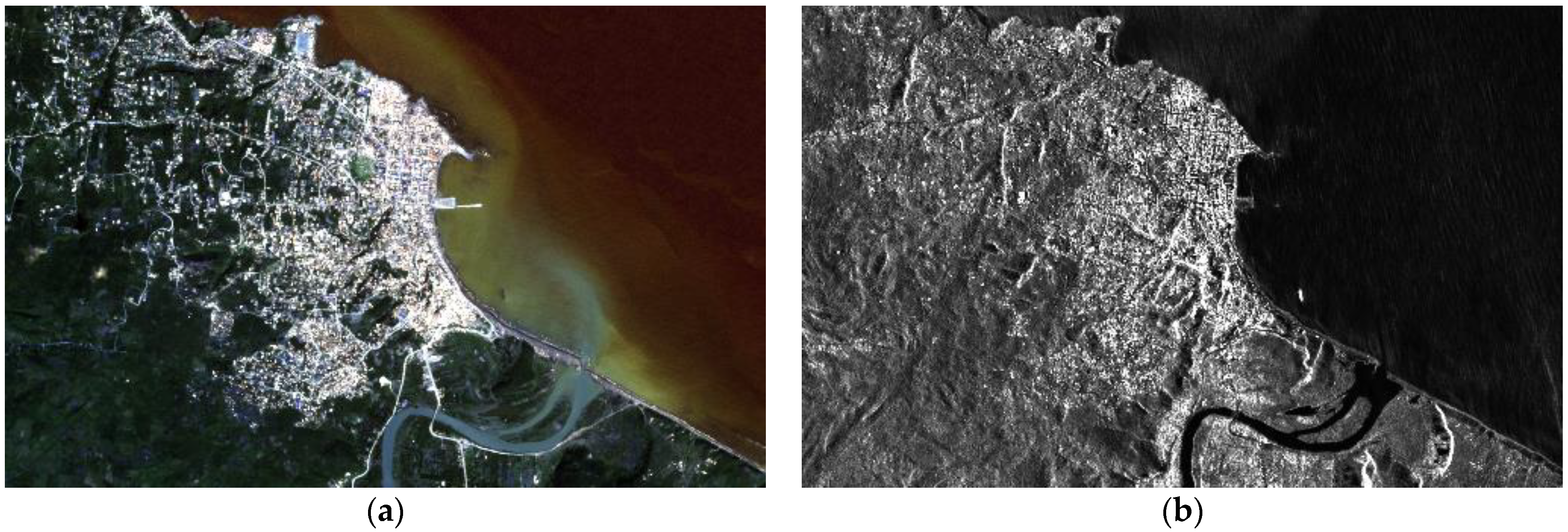
  • “Jérémie 2016”: Pansharpened Pléiades multispectral image (Figure 1) collected on 7 October 2016, i.e., few days after Hurricane Matthew hit the imaged area. The image is composed of 4 channels and has a pixel spacing of 0.5 m. The native resolution is 2 m for the multispectral channels and 0.5 m for the panchromatic channel.
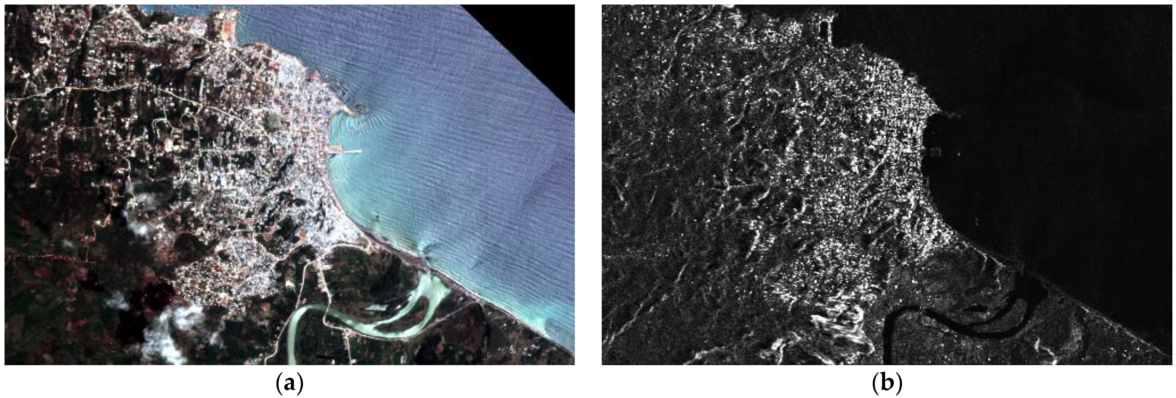
  • “Jérémie 2017”: Pléiades multispectral image (Figure 2a) collected on 18 October 2017, and composed of 4 channels with a native resolution of 2 m; COSMO-SkyMed Enhanced Spotlight right-looking image (Figure 2b) collected on 2 December 2016, with pixel spacing of 0.5 m, approximate spatial resolution of 1 m, and HH polarization.
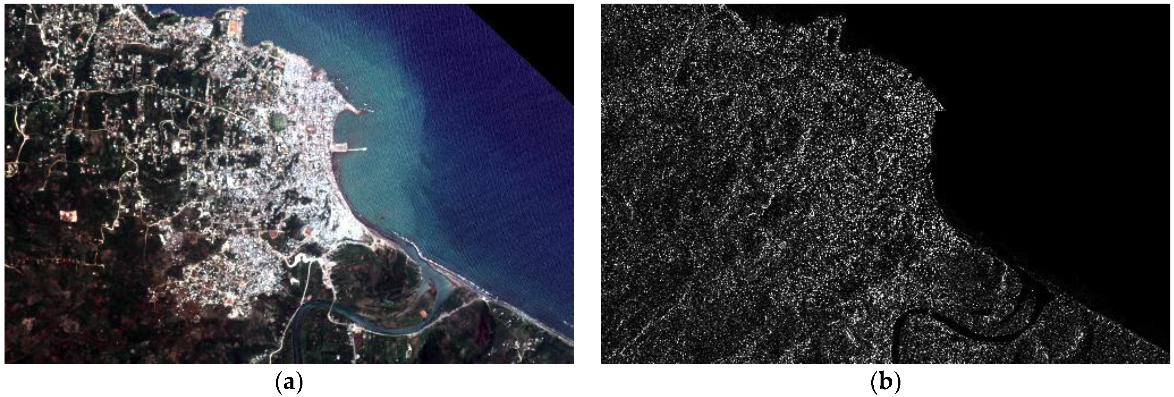
  • “Jérémie 2018”: Pléiades multispectral image (Figure 3a) collected on 24 April 2018, and composed of 4 channels with a native resolution of 2 m; COSMO-SkyMed StripMap HIMAGE right-looking image (Figure 3b) collected on 12 May 2018. The polarization is HH and the spatial resolution is approximately 3 m.
  • “Jérémie 2019”: Pléiades multispectral image (Figure 4a) collected on 15 March 2019, and composed of 4 channels with a native resolution of 2 m; COSMO-SkyMed Enhanced Spotlight right-looking image (Figure 4b) collected on June 20, 2019, with the same resolution of “Jérémie 2017”.
It is worth anticipating that the proposed method jointly generates a change map and two classification maps starting from data collected at two different dates. In the following, when more than one image (e.g., optical and SAR acquisitions) is available at a given date, they are listed as separated by a semicolumn. RGB compositions of the multispectral images and grey-scale displays of the SAR amplitude images are shown in Figure 1, Figure 2, Figure 3 and Figure 4.

3.2. Overview of the Proposed Method

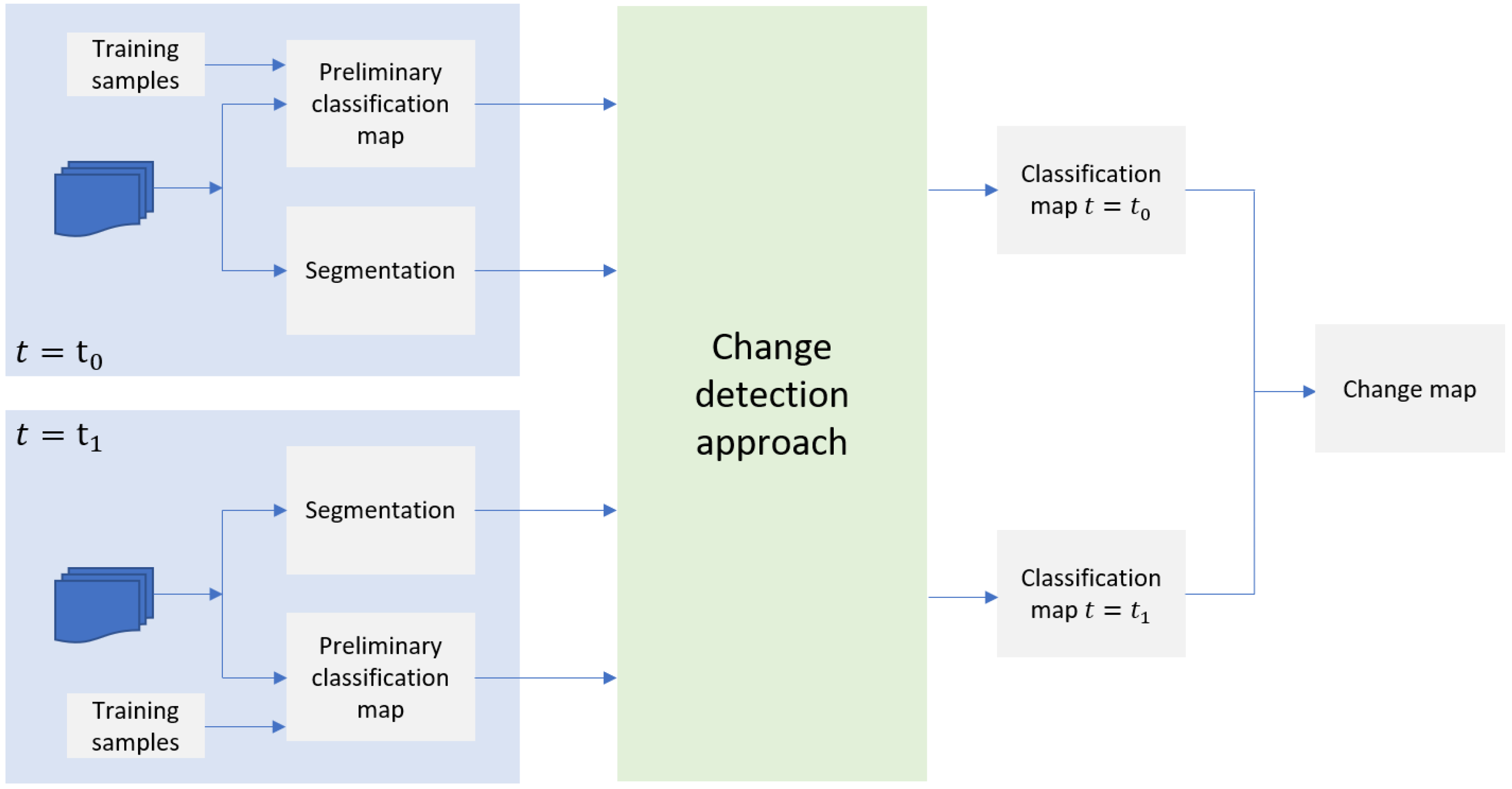
The proposed method generates a change map and two classification maps by modeling the spatial and temporal relationships within the input multitemporal and multisensor dataset via the regularization and data fusion capabilities of MRF modeling. The flowchart of the method is depicted in Figure 5. At both dates t 0 and t 1 , by using an available training set, a preliminary classification map is computed by means of kernel-based methods, ensemble methods, or other classifiers. As is shown later, the proposed framework is not sensitive to the choice of this initial classifier. Moreover, segmentation maps corresponding to multiple levels of detail are extracted from the input images. Then, the Markovian framework takes advantage of such a collection of data to jointly compute the two classification maps by modeling their spatiotemporal relationship. The change map, i.e., the map of class transitions from t 0 to t 1 , is finally computed based on the two classification results.
Due to the complexity of the input dataset, the straightforward application of the MAP decision rule for the joint computation of the two classification maps, and hence the change information, would be computationally intractable. Nevertheless, leveraging on the Hammersley–Clifford theorem and on the Markovian property of the prior probabilities, an energy minimization problem can be formulated as a computationally affordable solution to find the MAP estimate [5].
In particular, collecting all the image data in a matrix X and all the labels related to the thematic classes in a vector , the joint posterior distribution P ( | X ) is a Gibbs distribution and is proportional to the quantity exp [ U ( | X ) ] , where the energy U is defined locally according to the aforementioned neighborhood system. The Bayesian MAP rule is equivalent to the minimization of the energy U ( | X ) with respect to , given the input image X . Multiple information sources can also be fused in this Markovian framework by defining appropriate energy functions as linear combinations of contributions associated with the individual sources [43,59,60].

3.3. Energy Function of the Proposed Markov Model

The energy of the proposed MRF model takes into consideration three terms related to the spatial relationships between neighboring pixels, the temporal relationship between the acquisitions at different times, and the multiscale information conveyed by a region-based analysis of the input imagery.
Let us consider a multitemporal dataset defined over a pixel lattice I and composed of two images X 0 and X 1 acquired at times t 0 and t 1 , respectively, where t 0 < t 1 . Let us also suppose that the two images are well registered so that it is possible to process them coherently on the same reference frame. In the literature, many image registration methods exist [68,69,70], also capable of addressing multisensor registration problems [71,72,73].
Focusing on the image X r ( r = 0 , 1 ), the i th pixel of the pixel lattice I is represented by a feature vector x i r d r   of d r components. Moreover, denoting with Ω r = { ω k r : k = 1 , 2 , , K r } the set of thematic classes provided with training samples at time t r , the class label of the i th pixel is denoted as i r Ω r . Indeed, by assigning a class label to each pixel in the lattice I , it is possible to construct the label map r = { i r } i I .
The pair of label maps 0 and 1 indicates the possible class transitions occurring between times t 0 and t 1 . Indeed, the joint classification of the two images provides a solution to the change detection problem per se. Moreover, the changes are detected not only as a Boolean indication of changed and unchanged pixels, but also in terms of multiple transitions from/to different land covers at different dates. Examples may include the identification of the transitions among thematic classes such as urban areas, agricultural fields, grasslands, and forests.
A set S r = { S 1 r , S 2 r , , S Q r } of segmentation maps related to Q different scale levels is generated using the well-known Felzenszwalb and Huttenlocher’s segmentation method in [74,75]. It is a computationally efficient region-merging algorithm based on a graph representation of the input image.
Consistently with the Markovian approach to data fusion, the contextual spatial information related to each image, the temporal correlation between X 0   and X 1 , and the multiscale information provided by S r are fused together as a linear combination of different contributions to the energy function of the proposed MRF model:
U ( 0 ,   1 | S 0 ,   S 1 ,   X 0 ,   X 1 ) =           r = 0 1 [ i I q = 1 Q α q r ln P ( s i q r | i q r ) + β r i j P ( i r | j , 1 r )           + γ r i ~ j δ ( i r , j r ) ] ,
where the spatial and temporal neighborhood relations are indicated by i   ~   j and i j , respectively; s i q r represents the label of the i th pixel in the q th segmentation map S q r ( q = 1 , 2 , , Q ) ; and the parameters α q r , β r , and γ r represent the coefficients of the linear combination and weigh the various contributions to the MRF energy function.
In more detail, i   ~   j indicates that pixels i and j at the same date are neighbors with respect to a 4- or 8-connected spatial neighborhood. The notation i j means that i is a pixel in the image acquired at time t 0 , j is a pixel in the image collected at time t 1 (or vice versa), and either i and j correspond to the same spatial location or j belongs, in its own image, to the 4- or 8-connected neighborhood centered on the same location as i (see Figure 6). This relation defines a local neighborhood across the temporal pair of images. In other words, the relations ~ and define a spatiotemporal undirected graph across the pixel lattices of the two acquisitions at times t 0 and t 1 : each pixel at either t 0 or t 1 is a node of the graph, and there is an undirected edge between each pair of pixels i and j such that i j or i j . This graph, together with the Markovian formulation expressed by the proposed energy function, determines a multitemporal probabilistic graphical model for the relation among pixels at the same or at different times.
The energy function U ( ) is composed of unary and pairwise contributions. The former relates to the pixelwise terms, while the latter model the relations between pairs of neighboring pixels. The first term of the energy is a unary term defined according to the probability mass function (PMF) P k q r ( s ) = P { s i q r = s | i r = ω k r }   ( k = 1 , 2 , , K r ; q = 1 , 2 , , Q ; r = 0 , 1 ) of the considered segment labels conditioned to the thematic classes. It represents the energy contribution associated with each segmentation map S q r at time t r . The use of class-conditional PMFs in this role and their inclusion in the energy through negative logarithms are inspired by the analogous role of the class-conditional probability density functions of the feature vectors in classical MRF models for image classification and segmentation [5,9].
The PMF P k q r ( s ) can be estimated as a relative frequency, i.e., as the percentage of the pixels belonging to segment s in the segmentation map S q r and assigned to class ω k r over the total number of pixels assigned to ω k r   ( k = 1 , 2 , , K r ; q = 1 , 2 , , Q ; r = 0 , 1 ) . However, to perform this estimation, not only the stack of multiscale segmentation maps but also preliminary classification maps are necessary inputs at time t r ( r = 0 , 1 ). Accordingly, as a preliminary phase, each image X r is classified separately in a supervised manner using the training samples available at time t r ( r = 0 , 1 ). In general, this preliminary stage can be addressed using an arbitrary supervised classifier. In the proposed technique, a variety of methods has been considered:
  • The contextual classification method proposed in [76], which consists in a support vector machine (SVM) whose kernel function is based on a region-based approach and incorporates spatial information associated with an input segmentation map. The segmentation map associated with the finest scale among the aforementioned ones is used.
  • The framework proposed in [77] and extended in [78] that provides a rigorous methodological integration of the SVM and MRF approaches. It is based on a Hilbert space formulation, and its kernel combines the rationale of SVMs and a predefined spatial MRF model. The well-known Potts model is used in this role. The extensions in [78] also integrate global or near-global energy minimization algorithms based on graph cuts or belief propagation.
  • The random forest (RF) classifier, rooted in the ensemble learning theory. RF combines multiple individual decision trees, each trained on a random resampling of the training data (bagging) and using, at each decision node, a random subset of the full set of features.
The choice of these methods has been such that the set of classifiers considered for the preliminary phase of the proposed approach range from noncontextual (RF) to contextual methods based on both Markovian ([77,78]) and region-based formulations ([76]).
The second term of the linear combination in Equation (1) is the first pairwise contribution and models the temporal relationships. It is expressed in terms of transition probabilities P { i r = ω k r | j , 1 r = ω h , 1 r } from each thematic class ω h , 1 r at time t 1 r to each class ω k r at time t r ( r = 0 , 1 ). The transition probability obtained for the pair ( h , k ) represents the ( h , k ) -element of the K 1 r × K r transition probability matrix (TPM). Following the approach in [8], the expectation maximization (EM) method [79] is used to automatically estimate the TPM from the input pair of multitemporal observations, thus catching the temporal correlation between the two images. Details of this estimation process can be found in [8].
The last contribution in the MRF energy is again a pairwise contribution and models the spatial contextual information within the image collected at each time. It acts as a spatial regularizer by enforcing a smooth prior in the Bayesian formulation. It is integrated in the energy function through the Potts model [5].

3.4. Optimization of the Parameters and Energy Minimization

The parameters α q r , β r , and γ r in Equation (1) represent the weights of the energy contributions. Thanks to the linear model adopted in the proposed Markovian energy formulation, the estimation of such parameters can be performed using the method presented in [80]. This technique combines a minimum mean square error (MMSE) formulation with Platt’s sequential minimal optimization (SMO) algorithm. The technique in [80] formalizes the problem of the estimation of the weight parameters of the MRF model as a constrained quadratic optimization problem that is based on the correctness of the classification on the training set. SMO is well-known in the literature of quadratic programming for kernel machines (e.g., for SVM classification and regression) and is used here to numerically solve the aforementioned constrained quadratic problem. Algorithmic details can be found in [80].
Finally, the minimization of the proposed energy function is accomplished using the graph cut α - β swap algorithm [76]. The graph cut approach has been chosen due to its capability to obtain strong local energy minima in a computationally efficient manner [81,82]. Leveraging on the Ford–Fulkerson theorem, the graph cut method for binary classification is based on the reformulation of the energy minimization problem as a max-flow/min-cut problem over a suitable graph [83]. In this binary case, graph cuts allow reaching a global minimum in polynomial time. In the case of a multiclass classification setup, graph cut methods, such as the α - β swap algorithm, converge to a local minimum that is characterized by “strong” analytical properties with respect to suitable optimality criteria [81,82]. Intuitively, and according to [82], such a strong local minimum may be thought of as a local minimum in a “wide valley”. As compared to deterministic methods such as iterated conditional mode [84], which converges to a generic local minimum in a short time [5], or to stochastic methods such as simulated annealing, which converges to a global minimum but takes a very long time [6], the graph cut approach represents an effective solution from both viewpoints of accuracy and computational burden.

4. Results

The proposed approach has been applied to the case study described in Section 3.1 and associated with optical (Pléiades) and SAR (COSMO-SkyMed) data collected between 2016 and 2019 in the area of Jérémie, southwestern Haiti, in relation to the recovery after Hurricane Matthew.
Given the target spatial resolution of the output maps (10 m for all results and 2 m in specific cases; see Section 3.1), the input images have been subsampled onto the corresponding pixel grid, because the method produces classification results at the same resolution as the input data. Proper antialiasing has been applied within this subsampling preprocessing step. The proposed method has been applied by using five segmentation maps (i.e., by considering five spatial scales), generated from each input image, and by using the method in [76] as the baseline supervised classifier to be used in the estimation of the class-conditional PMFs. The results shown in the present section refer to this setup. We refer to Section 5 for a discussion of the sensitivity to the number of scales and to the choice of the baseline preliminary classifier.
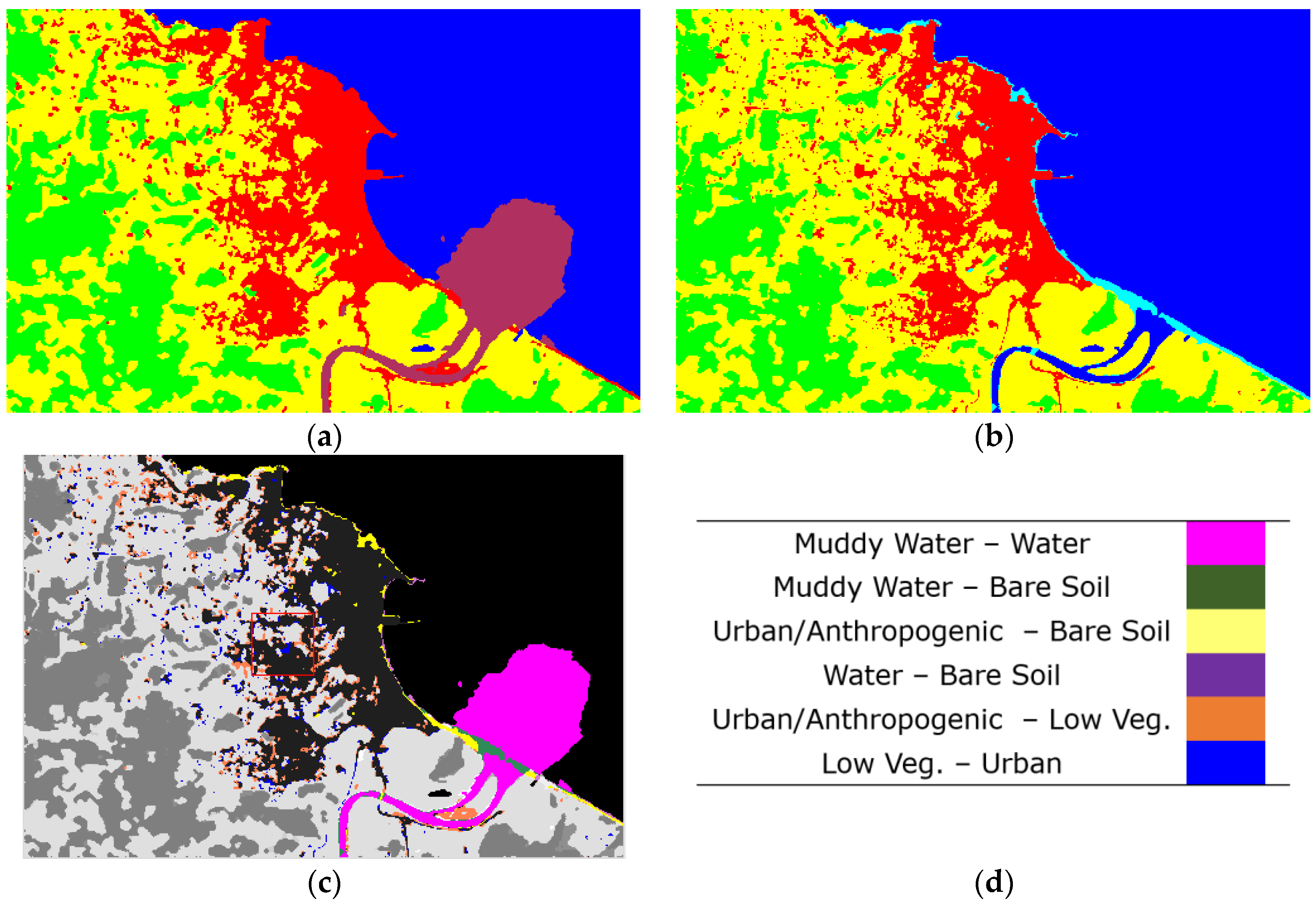
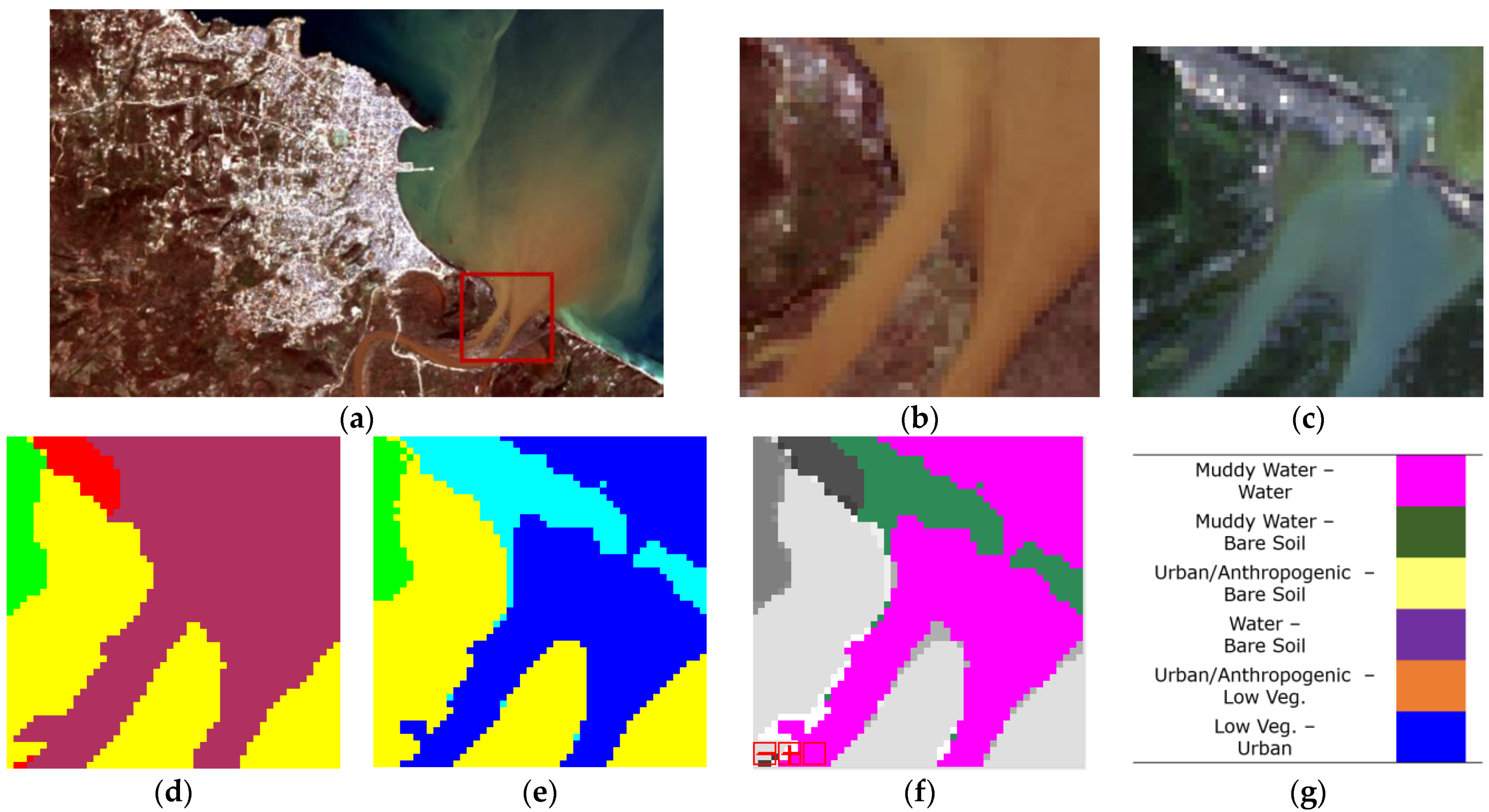
First, Figure 7 shows the outputs of the proposed method when applied at 10 m resolution to the pair of images “Jérémie 2016” and “Jérémie 2017”. The land cover classes include “urban/anthropogenic”, “tall vegetation”, “low vegetation”, and “water” in both imaged scenes and “muddy water” and “bare soil” in the cases of “Jérémie 2016” and “Jérémie 2017”, respectively. Intentionally, the labeling “urban/anthropogenic” is used to encompass the variety of changes occurring in Jérémie during the recovery phase due to urbanization—meant as the construction not only of new buildings but also of new infrastructures (e.g., roads)—and anthropogenic activities that alter the land cover (and thus the spectral reflectance and/or the radar backscatter) such as wastelands.
Figure 7 includes the classification map for 2016 (Figure 7a), the classification map for 2017 (Figure 7b), the change map highlighting the changes that occurred in the considered time window (Figure 7c), and the legend of the change map (Figure 7d). In this legend, colors indicate changes and shades of grey denote unchanged pixels belonging to the various classes. Table 1 shows the accuracy of the test samples for these classification maps. The table also specifies the legend used in the classification maps of Figure 7a,b. Discussion on the classes and class transitions that the method was able to identify is presented in Section 5.
The same set of experiments has also been carried out considering all pairs of datasets acquired in consecutive pairs of years between 2017 and 2019. In this case as well, the optical and SAR images have been downsampled to the resolution of 10 m. The resulting set of multitemporal classification maps contributes to the monitoring of the recovery phase after the hurricane.
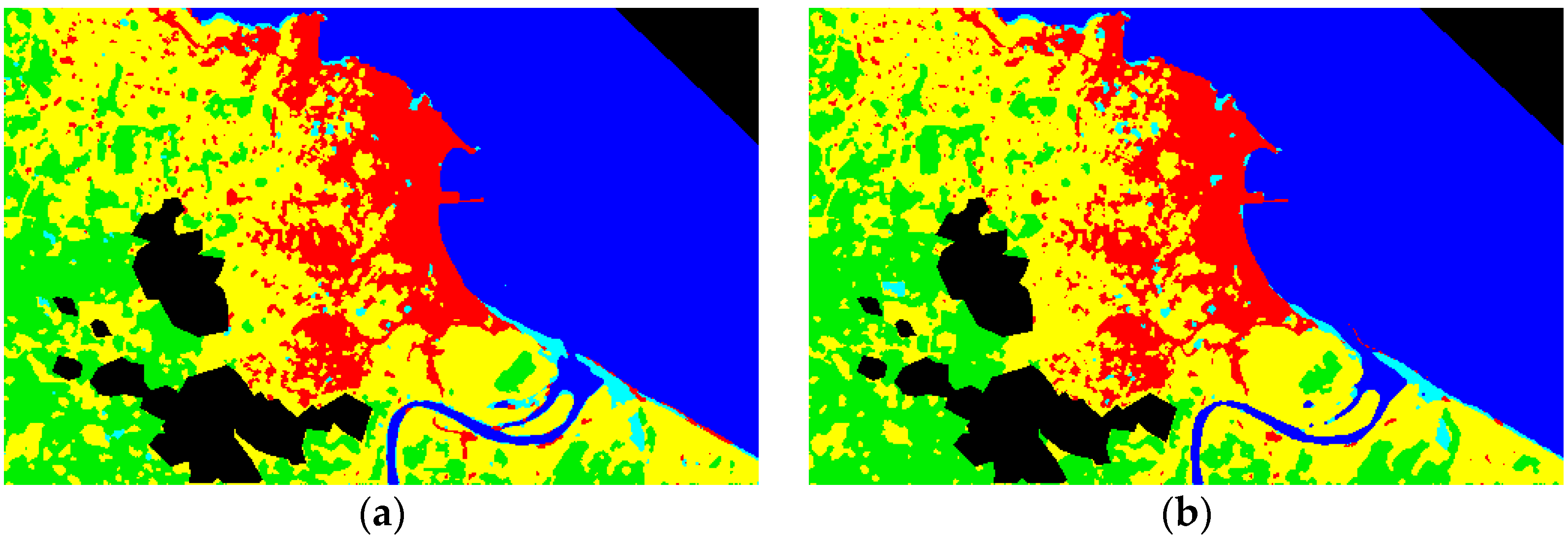
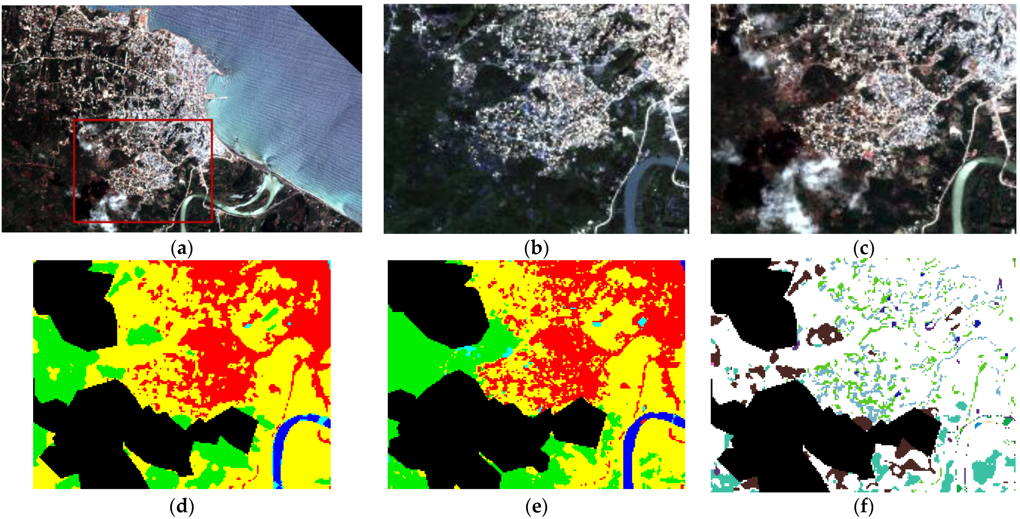
Figure 8 shows the classification maps obtained with pairs of datasets collected in 2017, 2018, and 2019. The classes are the same as in the case of 2017 (Figure 7). The proposed method jointly computes a couple of classification maps based on data collected at two different dates. Therefore, the same classification map is obtained more than once, from distinct temporal pairs. An example is the map of 2018, which is computed considering either the data of 2017 and 2018 or the data collected in 2018 and 2019. The same comment holds in the case of the map of 2017. However, the differences between the two maps generated for the same year were minor in all the cases, so, for the sake of brevity, we report only a single case, i.e., the map coming from the pair (“Jérémie 2016”, ”Jérémie 2017”) for 2017 and the map from the pair (“Jérémie 2017”, ”Jérémie 2018”) for 2018.
With regard to these classification results, Figure 9 shows the corresponding change maps, while Table 2 summarizes the accuracy scores. In this case, the thematic and change maps show unclassified areas, which correspond to parts of the input image that were covered by clouds in the Pléiades data and were therefore masked out. Such a masking operation has been chosen as a simple preprocessing step enabling the straightforward applicability of the proposed method to the application of recovery monitoring. Other solutions are indeed possible, such as missing data reconstruction techniques based on Bayesian or neural approaches [85,86]. The legends are shown in Figure 9 and Table 2.
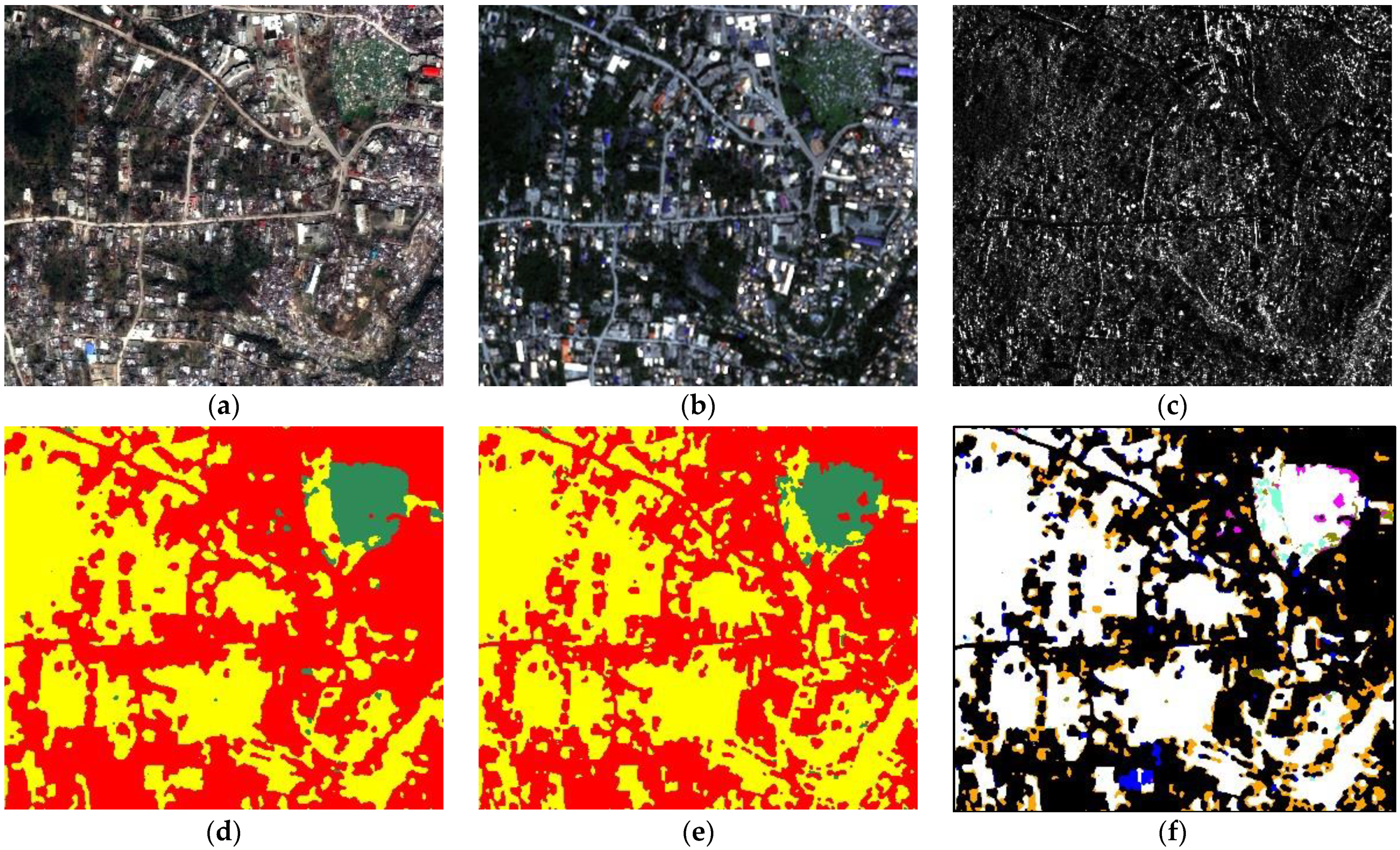
The results shown so far have been generated at the target spatial resolution of 10 m. To prove the capability of the proposed method to generate results at a finer resolution, a zoomed detail of the same area has also been classified at the resolution of 2 m. The images used for this dedicated experiment are those collected in 2016 and 2017.
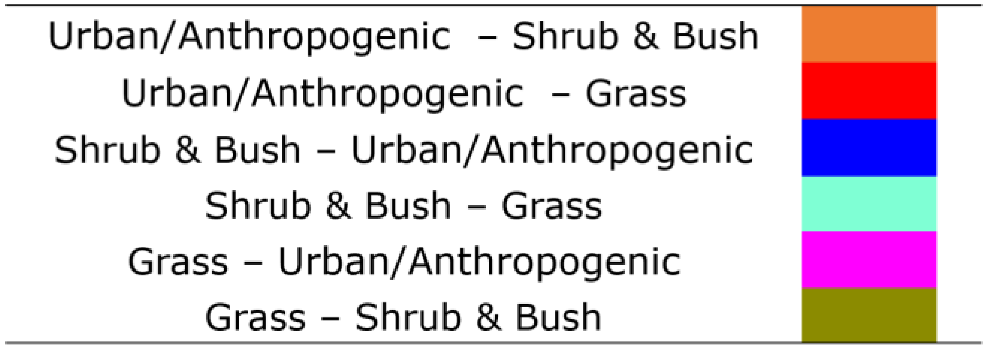
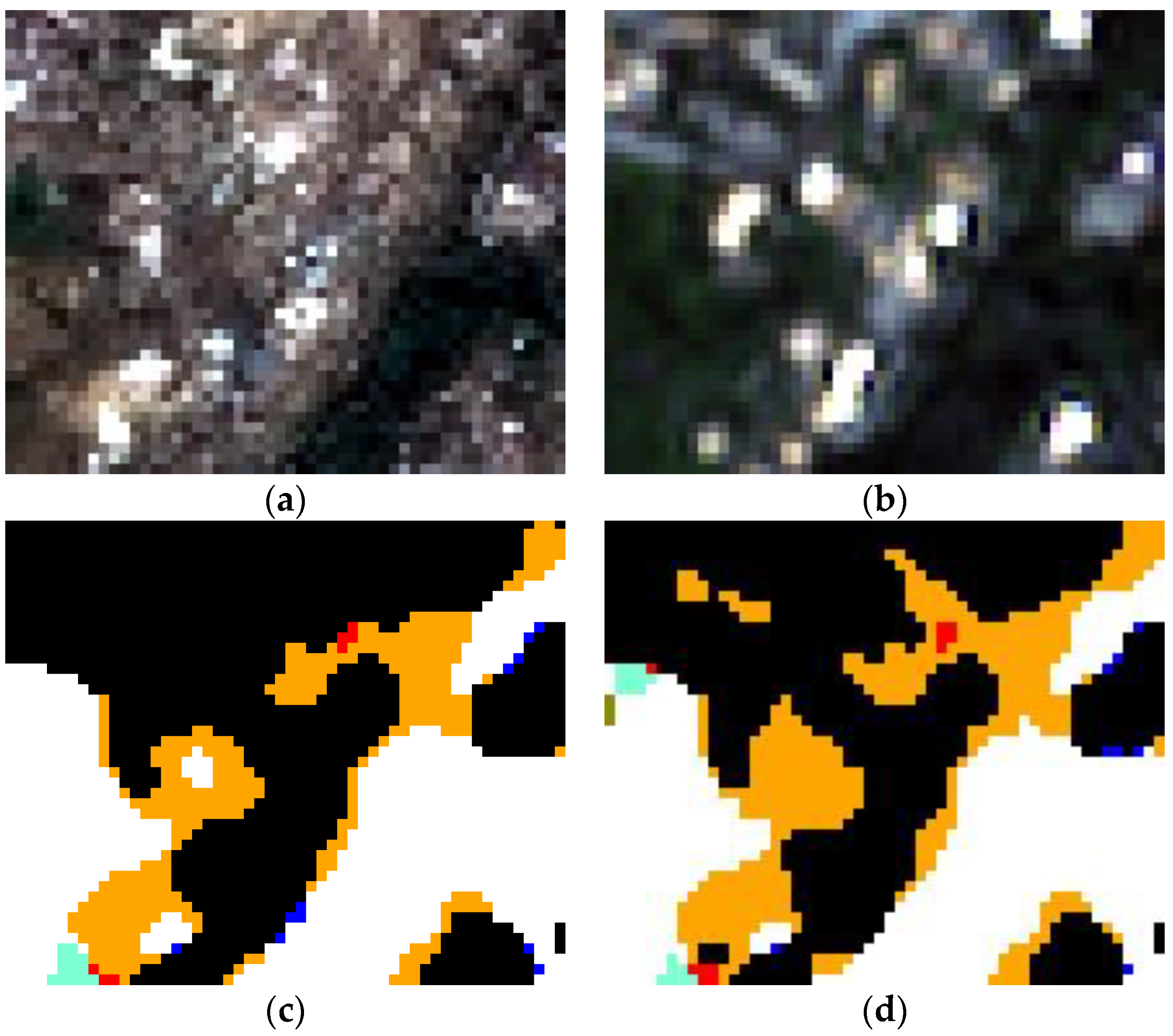
The zoomed area has been selected in the urban region of Jérémie, west of the main town cemetery. This choice has been driven by the possibility of using the high spatial details of the urban areas to assess the capability of the proposed method to generate effective products also at finer resolutions. The classes that can be appreciated in this zoomed area at 2 m resolution are “urban/anthropogenic” (in this case most exclusively due to the urban footprint and residential buildings), “grass”, and “shrubs and bush”, consistently with the finer level of spatial detail than in the aforementioned 10 m imagery. Indeed, the qualitative analysis of the maps in Figure 10, together with the quantitative evaluation of the scores summarized in Table 3, confirm the absence of oversmoothing effects and artifacts due to the Markovian modeling. Conversely, the maps show a remarkable homogeneity in the areas of the same land cover class. The discussions on the classes and class transitions in this case of higher-resolution input data are also provided in Section 5.

5. Discussion

In Section 4, we have presented the experimental results achieved by the proposed method on the datasets spanning the time window that ranges from 2016 to 2019. Here, the focus is on the discussion of such results and of the behavior of the proposed method with respect to the related model selection issues. Since the weight parameters in the energy function are automatically optimized, these issues regard the number Q of segmentation levels and the choice of the baseline classifier used for the generation of the preliminary thematic maps. Another point that is addressed is related to the multisensor fusion capabilities. The method fuses multisensor optical–SAR acquisitions at two different dates for classification purposes. Hence, an ablation study, in which the multitemporal classification is performed using both optical and SAR data as compared to optical data only, is presented to assess the importance of the radar component with respect to the classification capabilities. Multispectral data are well known to be usually a very informative source of information for the classification of heterogeneous land cover types. Nevertheless, SAR data can be very useful for the discrimination of a subset of such classes, such as urban areas and water bodies. The ablation study is aimed precisely at appreciating the added value of the SAR component in the output results of the proposed approach. Finally, the change maps are analyzed by assessing their capability of identifying land cover transitions that are typical of the recovery phases in the aftermath of natural disasters.
Starting from the results obtained on the 10 m resolution dataset of 2016 and 2017 (see Figure 7), the most relevant transition is the one highlighting the “muddy water” turning into clean “water” in the area close to the mouth of the Grande Anse River. This is in line with the recovery of the natural riverine and coastal environments from the dramatic situation imaged in 2016, just a few days after the hurricane.
A second type of change indicates the rise of a “bare soil” area at the mouth of the river in 2017 (Figure 12) and still existing in 2019 (Figure 13). Such a formation was not present in the period immediately after the disaster. The change detection method therefore was able to document and spatially locate another typical natural process that, in the case of Jérémie, was found to have interesting implications for the local community economics and subsistence. At the time of the ground-truth validation in April 2019, the new river mouth bar and the rejuvenated coastline (Figure 13c) were exploited as a natural commodity by local inhabitants to source sand and gravel to be used as building construction materials (Figure 13d). This adds to the evidence of quarrying activities that developed later in 2018–2019 in the nearby hills, a few hundred meters to the south, as highlighted by the 2019 classification map in the form of a pixel cluster of land cover transition due to “anthropogenic” activity and not “urbanization” in a strict sense (see black circle in Figure 13b).
Moreover, in the coastal area, some “urban/anthropogenic” and “water” areas have turned into “bare soil” areas (i.e., yellow and purple pixels in the change map). While the ground-truth data corroborate the accuracy of this change detection classification, they also confirm that the sand and gravel are interspersed with widespread rubbish and waste (Figure 13c), which contributed to a spectral heterogeneity of the “bare soil” class.
Finally, another type of transition that has been identified involves the mutual change between “urban/anthropogenic” and “vegetated” areas (i.e., orange and blue pixels in the change map). As mentioned in Section 4, at the considered resolution, the class “urban/anthropogenic” is spatially heterogeneous and composed of a set of subclasses (including some types of “wasteland” areas), which makes the related classification process a challenging task.
Considering the experiments with data collected in the subsequent years (i.e., the “Jérémie 2017”, “Jérémie 2018”, and “Jérémie 2019” datasets), the changes that have been identified involve primarily “vegetation” and “urban/anthropogenic” areas. Figure 14 zooms onto the southwestern sector of Jérémie and the related details of the classification and change maps resulting from the 2017–2018 temporal pair. The vast majority of transitions involve “tall” and “low vegetation”. On one hand, this is related to the fact that the two acquisitions are temporally located in two different seasons (i.e., autumn and spring), thus leading to a change in the vegetation present in the scene. On the other hand, at the resolution of 10 m, the textural details of the remotely sensed images do not well characterize the typical features of the vegetation, thus hampering correct discrimination of different vegetation types.
Conversely, the transitions from “vegetated” areas to “urban/anthropogenic” areas that are identified are correlated with the reconstruction efforts of the recovery phase, as was ascertained during the validation survey in April 2019. Such increase in residential buildings mostly occurred across a hilly and quite steep area of the town, where a parallel investigation with multitemporal interferometric SAR (InSAR) techniques [67] relying on Sentinel-1 scenes in the period 2017–2018 highlighted the presence of ground motions in the direction away from the satellite sensor (velocity of up to −2.4 cm/year). As emerged during the two user workshops organized by CNES and CNIGS with the Haitian partners and stakeholders in Jérémie and Port-au-Prince in April–May 2019, such a combination of geospatial information represents relevant information for local and national authorities in their efforts to monitor the recovery phase, prevent new exposure to hazards, and implement resilient land use policies [87].
All the comments above refer to the results obtained from input data downsampled to 10 m. Regarding the results at 2 m resolution, most of the transitions that have been identified involve the “urban/anthropogenic” and “vegetation” classes. In the change map in Figure 10f, the blue transitions (from “vegetation” to “urban/anthropogenic”) suggest rebuilding operations that have been conducted after the disaster. It is common that some pixels showing highly damaged buildings were classified as “bare soil” or “vegetation” in 2016. Conversely, the transitions from “urban/anthropogenic” to “vegetation” (orange in Figure 10f) may indicate areas that were so damaged that the old buildings have been dismissed and replaced by green areas.
Concerning the classification of urban areas, it is well known from the literature [88] that SAR data are usually informative for the discrimination of this class. Moreover, the case reported above with VHR data is particularly challenging in this perspective due to the spatial heterogeneity and the presence of multiple subclasses in the urban scene. Nevertheless, the proposed method effectively discriminates the built-up areas in the scene by taking advantage of both multispectral optical and SAR data. To assess the importance of the COSMO-SkyMed data, Figure 15 shows a comparison of the results obtained with and without input COSMO-SkyMed imagery. The figure focuses on an example of detail of the 2016–2017 temporal pair. Figure 15c shows the change map generated using the multispectral optical dataset only, while Figure 15d shows the result obtained by integrating both optical and radar data. It is straightforward to qualitatively appreciate the visual impact of the second source of information on the effective discrimination of the changes, and thus the correct classification of the challenging “urban” pixels. In this case as well, the legend is the one reported in Figure 10c.
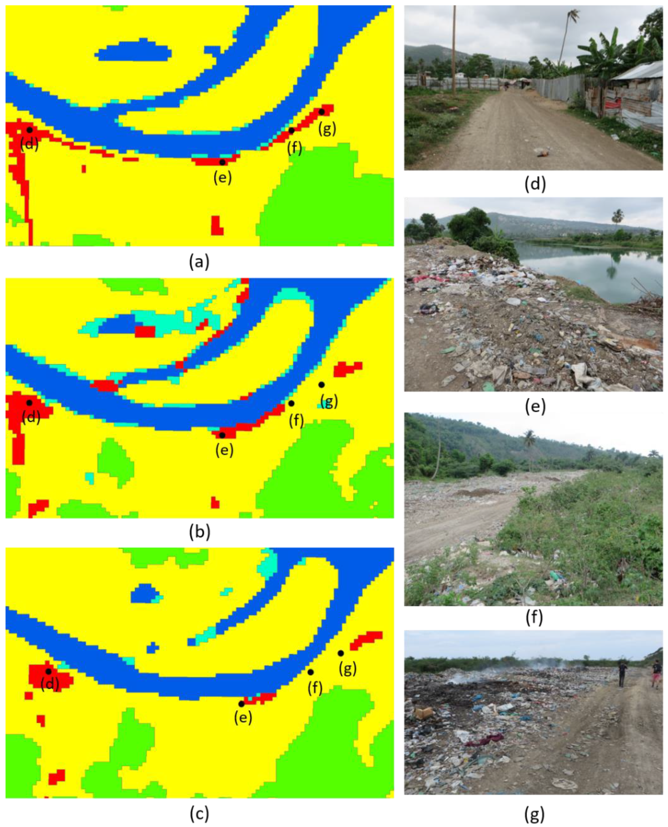
With regard to “urban/anthropogenic”, SAR also helps to capture other land cover transitions that are associated with anthropogenic impact (e.g., wasteland, dump sites) that may be confused due to spectral heterogeneity if multispectral optical data were used alone. However, the interpretation of the cause of such a land cover transition could not be so straightforward without some knowledge about the condition on the ground. This was evident during the validation of “urban/anthropogenic” changes found in the classification map corresponding to 2017 along the right bank of the Grande Anse River, south of Jérémie (Figure 16). These changes were not due to building construction as the “urban” classification would suggest, but rather wasteland as unregulated and uncontrolled open-air dump sites (Figure 16e,f), where garbage, plastic, and different types of solid waste are accumulated and, sometimes, even burnt (Figure 16g).
The issue of piles of solid wastes by roadsides, rivers, and other open spaces associated with the expansion of urban areas and lack of city planning in Haiti (particularly Port-au-Prince), thus causing significant health and environmental problems, was already reported in the literature [89] and URD’s Observatory in Haiti [90]. The developed change detection method was able to detect that such change already occurred in the first year after the hurricane. On the contrary, the classification map corresponding to 2019 seemed to highlight that most of the dump area transitioned to “low vegetation” (Figure 16c), whereas in situ inspection confirmed that this area was still present (Figure 16e,g). The waste burning and the growth of vegetation have likely led the classifier to confuse the local spectral response and thus output such a classification result.
For sure, this example reassures about the importance of undertaking multitemporal change detection through regularly spanned satellite observations across the whole duration of the recovery phase (i.e., from near to long term), the wise choice to adopt a wide concept of the “urban/anthropogenic” class given its heterogeneity, and the opportunity to validate the classification results vs. the current context on the ground. A correct interpretation of land cover transitions also has a direct impact on the possible use of these classification maps in risk assessment and reduction. The assumption that the changes found along the river were due to urban constructions may have led to the wrong assessment about an increase in the elements at risk, for instance, of flooding events or hurricanes. On the contrary, the detected land cover changes warn about an anthropogenic process associated with the recovery process, which causes an increase in local hazards to both the environment and the health of the local community.
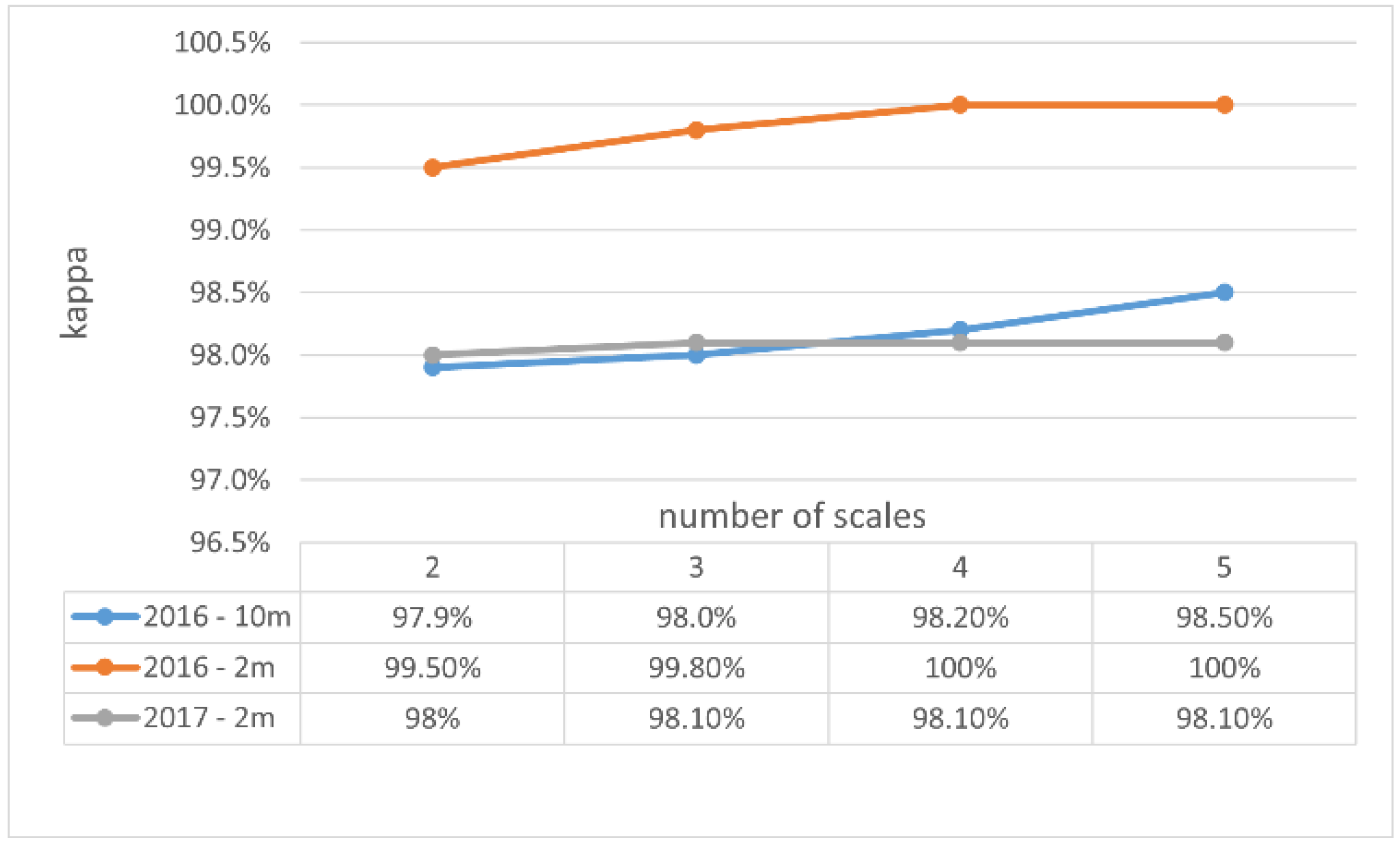
Concerning the behavior of the method as a function of the number Q of segmentation levels, Figure 17 displays the Cohen’s κ of different classification maps as a function of Q . Here, the maps that are being considered are the ones corresponding to 2016 at 10 m and those of 2016 and 2018 at 2 m. The performances do not vary much as the number of scales is increased from 2 to 5. On one hand, this result confirms the stability of the output products with respect to the parameter Q , thus suggesting that the choice of its value is not critical. On the other hand, according to common practice in remote sensing, the test pixels are located inside homogeneous areas to minimize the impact of mixed pixels on accuracy assessment. Nevertheless, all the maps shown in Section 4 suggest a regular behavior at the interface between adjacent classes without artifacts or oversmoothing effects.
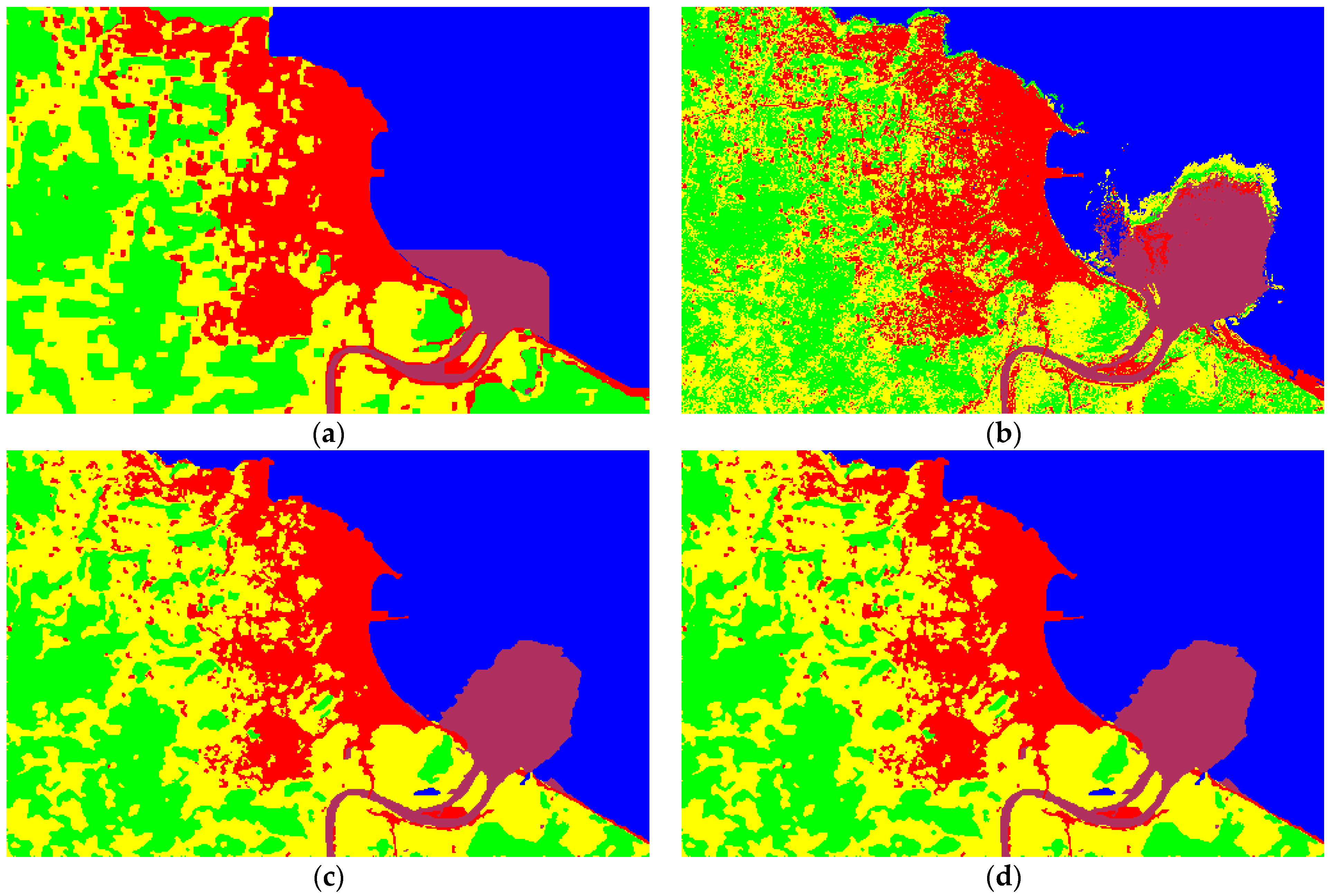
Concerning the behavior of the proposed method as a function of the preliminary supervised classifier used in the estimation of the class-conditional PMFs, Figure 18 displays examples both of preliminary classification maps obtained via different baseline classifiers and of the output maps of the proposed technique. In addition to the aforementioned results, which were based on the use of the method in [76] for the preliminary classification stage, RF and the method in [78] are addressed in this example. The higher accuracy granted in the preliminary stage by the contextual algorithm in [78] than by the noncontextual RF can be noted by comparing Figure 18a,b. Nevertheless, it can be immediately seen that the final maps of the proposed Markovian method are mostly identical to each other and to the map in Figure 7a (which was obtained by starting from the preliminary map generated by the technique in [76]). This suggests the very limited sensitivity of the Markovian fusion framework to the baseline classifier considered for the initialization.
This robustness can be interpreted in terms of the role of the preliminary classification maps within the overall proposed method. Indeed, the preliminary maps are used to estimate the class-conditional distributions P ( s i q r | i q r ) of the segment labels at all considered scales (see Equation (1)). So, first, they affect only the multiscale terms of the energy function in Equation (1), whereas the temporal and spatial terms are unaffected. Then, the multiscale energy terms are also associated with a stack of segmentation maps, which, in turn, are generated independently from the preliminary classification maps. The use of the segmentation maps implies a remarkable spatial regularization in the estimates of the class-conditional distributions P ( s i q r | i q r ) . This spatial regularization significantly mitigates the possible impact of the specific choice of the preliminary classification maps on the energy function of the proposed MRF model—and in turn on the resulting energy minimum identified using graph cuts. Nevertheless, it is worth noting that the initial classification maps in Figure 18a,b are overall consistent. They differ in the discrimination of low/tall vegetation and of the urban/anthropogenic areas and especially in the shape of the detected region of muddy water region (see Figure 18). However, as described above, such differences do not significantly affect the output of the Markovian modeling.
In particular, as pointed out again by Figure 18, the proposed method is able to generate more accurate classification maps than the pixelwise RF classifier and the contextual method in [78] combining SVM and MRF. The classification errors made by the method in [78] and by RF are evident in Figure 18a,b, respectively, as compared to the maps obtained by the proposed approach in panels (c) and (d). For instance, the map of RF in panel (b), which corresponds to an overall accuracy of around 79%, looks quite noisy, which is in accordance with the fully noncontextual formulation of this classifier. However, the proposed method generally demands more computational resources than the considered previous techniques. Nevertheless, such an increased computational burden is not dramatic, especially in relation to the aforementioned gain in accuracy and to the addressed goal. For example, on the 2016–2017 dataset, RF required around 3 min to generate the two classification maps, while the contextual method in [78] and the SVM with region-based kernel in [76] required around 8 min. Conversely, the proposed method, given the input preliminary maps generated with one of the aforementioned algorithms, took a time ranging from 9 to 15 min depending on the number of scales (ranging from 2 to 5). The machine used for the experiments was a laptop equipped with an i73632QM processor working at a maximum frequency of 3.6 GHz and 8 GB of DDR3 RAM. The times taken in the cases of the other image pairs were similar. In particular, the goal of the considered approach is to map land-cover changes to monitor the recovery effort after Hurricane Matthew. It is worth noting that, compared to the timescale of a recovery process, the computation time of the proposed approach is very short; i.e., there are no computational criticalities in relation to the addressed application.

6. Conclusions

A novel method has been proposed in this paper to address the problem of supervised multitemporal joint classification of multisensor optical–SAR images in the framework of the application to the monitoring of the recovery phase after Hurricane Matthew in Haiti. The method makes use of a probabilistic graphical approach formulated through a novel MRF model. This model integrates spatial and temporal relations as well as multiscale information associated with segmentation maps considering different levels of detail.
The method has been applied to and validated in the CEOS Haiti RO test area of Jérémie. The experimentation involved Pléiades and COSMO-SkyMed data collected in the period ranging from 2016 to 2019. From an application viewpoint, the proposed method proved to be accurate in the discrimination of the land cover classes in the considered scene. In particular, the land cover transitions that have been detected are consistent with the presence of rebuilding activity, the removal of damaged buildings in favor of green areas, and seasonal changes in the vegetation of the area. The output classification maps also highlighted areas of land cover transition to “bare soil”, at the mouth of the Grande Anse River and along the coast, as well as to “urban/anthropogenic” along the right riverbank. These areas are related to anthropogenic activities of mining, quarrying, and waste disposal that represent some of the social, cultural, and economic facets of the recovery process in Jérémie. The obtained results confirm the potential of MRF-based approaches in applications to remote sensing analysis tasks involved in the management of natural disasters and risk reduction [91,92].
Consistently with the requirements of the general context of this study, which was framed within the CEOS Haiti RO initiative, the mapping was mainly focused on 10 m spatial resolution. However, the challenging scenario of VHR data at 2 m resolution has also been analyzed, pointing out the effectiveness of the proposed approach in this case as well and the usefulness of the input SAR data in the discrimination of the urban area.
From a methodological viewpoint, the experimental validation also addressed the sensitivity of the proposed technique with respect to the related model selection issues. In particular, the performances of the method exhibited remarkable stability as the number of input segmentation maps was varied and as a function of the preliminary classification maps involved in the calculation of the unary energy contributions. This suggests that the configuration of the method is not a critical phase and confirms its applicability in the addressed recovery monitoring framework. In particular, among the baseline classifiers that have been considered, both a well-known noncontextual algorithm (random forest) and three contextual techniques of various complexities have been experimentally evaluated. The very low impact of the choice of this preliminary classification stage on the performances of the proposed approach suggests using the most time-efficient baseline method among the considered ones, i.e., random forest. Indeed, this limited sensitivity is consistent with the fact that the preliminary maps are used only to determine one of the components of the energy of the proposed MRF, whereas the output land-cover change result is determined by fusing this information with spatial, temporal, and multiscale contributions.
From this perspective, an interesting future extension of this work will consist in further extending the spatial modeling capabilities of the proposed approach by also combining it with CNN architectures [61]. On one hand, this is expected to favor a further improvement in classification performances. On the other hand, it will generally imply stricter requirements in terms of ground truth. In this respect, similar to [93,94], the combination of MRF/CRF and CNN models could be specifically aimed at mitigating the need for especially large training sets, typical of deep learning techniques. Furthermore, in the conducted case studies, cloud-covered portions of the imaged scene were masked out directly. As a further generalization, missing data reconstruction methods, based for instance on Bayesian or deep neural approaches [85,86], could be integrated in the developed approach to benefit from the available satellite image time series and fill the gaps due to the presence of clouds.
From an application viewpoint, the effectiveness demonstrated by the proposed approach in the case study on Jérémie, Haiti, suggests its extension to other multitemporal processing tasks associated with disaster risk management, including, for instance, the update of land cover maps in the assessment of the vulnerability of a given area or the detailed mapping of the ground changes after an event occurs.

Author Contributions

Conceptualization, D.T., G.B. and S.Z.; data curation, A.D.G.; formal analysis, A.D.G., D.S., G.M. and S.B.S.; funding acquisition, G.M., D.T., G.B., R.R., S.B.S., A.R.P., A.M. and S.Z.; investigation, A.D.G., G.M., D.T., F.C., G.B. and R.R.; methodology, A.D.G., G.M., and S.B.S.; project administration, G.M., D.T., G.B., R.R., S.B.S., A.R.P., A.M. and S.Z.; resources, D.T., G.B., R.R. and S.Z.; software, A.D.G.; supervision, G.M., G.B. and S.B.S.; validation, A.D.G., G.M., D.T. and F.C.; visualization, A.D.G., D.S., D.T. and F.C.; writing—original draft, A.D.G., D.S., G.M., D.T. and F.C.; writing—review and editing, A.D.G., D.S., G.M., D.T., F.C., G.B., R.R., S.B.S., A.R.P., A.M. and S.Z. All authors have read and agreed to the published version of the manuscript.

Funding

This research was carried out within the project “CEOS Disaster Risk Management (CEOS DRM)”, funded by the Italian Space Agency (ASI) and framed within the agreement No. 2017-24-H.0 between ASI and CIMA Foundation. The support is gratefully acknowledged.

Acknowledgments

Pléiades and COSMO-SkyMed data were provided by CNES and ASI, respectively, in the framework of the CEOS Haiti RO project. The authors would like to thank ASI and CNES for providing these data. They also greatly acknowledge Alessandro Montaldo for his help in conducting part of the experiments, Boby Emmanuel Piard and his collaborators at CNIGS, Samuel Généa (Bureau des Mines et de l’Énergie—BME), Hélène de Boissezon and Agwilh Collet (CNES), and Robin Faivre (SERTIT) for their collaboration and support to ASI researchers during the technical mission in Haiti for ground-truth validation.

Conflicts of Interest

The authors declare no conflict of interest.

References

  1. The Recovery Observatory in Haiti in Short. Recovery Observatory Haiti by CEOS. Available online: https://www.recovery-observatory.org/drupal/en (accessed on 28 June 2021).
  2. Haiti RO for Hurricane Matthew Recovery|CEOS|Committee on Earth Observation Satellites. Available online: https://ceos.org/ourwork/workinggroups/disasters/recovery-observatory/haiti-ro-for-hurricane-matthew-recovery/ (accessed on 14 May 2021).
  3. Bovolo, F.; Bruzzone, L. The Time Variable in Data Fusion: A Change Detection Perspective. IEEE Geosci. Remote Sens. Mag. 2015, 3, 8–26. [Google Scholar] [CrossRef]
  4. Solberg, A.; Taxt, T.; Jain, A. A Markov random field model for classification of multisource satellite imagery. IEEE Trans. Geosci. Remote Sens. 1996, 34, 100–113. [Google Scholar] [CrossRef]
  5. Li, S.Z. Markov Random Field Modeling in Image Analysis; Springer Science & Business Media: Berlin/Heidelberg, Germany, 2009. [Google Scholar] [CrossRef]
  6. Geman, S.; Geman, D. Stochastic Relaxation, {G}ibbs Distributions, and the {B}ayesian Restoration of Images. IEEE Trans. Pattern Anal. Mach. Intell. 1984, PAMI-6, 721–741. [Google Scholar] [CrossRef]
  7. Moser, G.; Serpico, S.B.; Benediktsson, J.A. Land-Cover Mapping by Markov Modeling of Spatial–Contextual Information in Very-High-Resolution Remote Sensing Images. Proc. IEEE 2012, 101, 631–651. [Google Scholar] [CrossRef]
  8. Moser, G.; Serpico, S.B. Multitemporal region-based classification of high-resolution images by Markov random fields and multiscale segmentation. In Proceedings of the 2011 IEEE International Geoscience and Remote Sensing Symposium, Vancouver, BC, Canada, 25–29 June 2011; pp. 102–105. [Google Scholar] [CrossRef]
  9. Kato, Z. Markov Random Fields in Image Segmentation. Found. Trends Signal Process. 2011, 5, 1–155. [Google Scholar] [CrossRef]
  10. Blaschke, T. Object based image analysis for remote sensing. ISPRS J. Photogramm. Remote Sens. 2010, 65, 2–16. [Google Scholar] [CrossRef] [Green Version]
  11. De Giorgi, A.; Moser, G.; Boni, G.; Pisani, A.R.; Tapete, D.; Zoffoli, S.; Serpico, S.B. Recovery Monitoring in Haiti After Hurricane Matthew Through Markov Random Fields and a Region-Based Approach. In Proceedings of the IGARSS 2019—2019 IEEE International Geoscience and Remote Sensing Symposium, Yokohama, Japan, 28 July–2 August 2019; pp. 9357–9360. [Google Scholar] [CrossRef]
  12. Singh, A. Digital change detection techniques using remotely-sensed data. Int. J. Remote Sens. 1989, 10, 989–1003. [Google Scholar] [CrossRef] [Green Version]
  13. Coppin, P.; Jonckheere, I.; Nackaerts, K.; Muys, B.; Lambin, E. Review ArticleDigital change detection methods in ecosystem monitoring: A review. Int. J. Remote Sens. 2004, 25, 1565–1596. [Google Scholar] [CrossRef]
  14. Lu, D.; Mausel, P.; Brondízio, E.; Moran, E. Change Detection Techniques. Int. J. Remote Sens. 2004, 25, 2365–2401. [Google Scholar] [CrossRef]
  15. Radke, R.J.; Andra, S.; Al-Kofahi, O.; Roysam, B. Image change detection algorithms: A systematic survey. IEEE Trans. Image Process. 2005, 14, 294–307. [Google Scholar] [CrossRef]
  16. Johnson, R.D.; Kasischke, E.S. Change vector analysis: A technique for the multispectral monitoring of land cover and condition. Int. J. Remote Sens. 1998, 19, 411–426. [Google Scholar] [CrossRef]
  17. Sziranyi, T.; Shadaydeh, M. Segmentation of Remote Sensing Images Using Similarity-Measure-Based Fusion-MRF Model. IEEE Geosci. Remote Sens. Lett. 2014, 11, 1544–1548. [Google Scholar] [CrossRef] [Green Version]
  18. Bazi, Y.; Bruzzone, L.; Melgani, F. An unsupervised approach based on the generalized Gaussian model to automatic change detection in multitemporal SAR images. IEEE Trans. Geosci. Remote Sens. 2005, 43, 874–887. [Google Scholar] [CrossRef] [Green Version]
  19. Hedhli, I.; Moser, G.; Zerubia, J.; Serpico, S.B. New cascade model for hierarchical joint classification of multitemporal, multiresolution and multisensor remote sensing data. In Proceedings of the 2014 IEEE International Conference on Image Processing (ICIP), Paris, France, 27–30 October 2014; pp. 5247–5251. [Google Scholar] [CrossRef] [Green Version]
  20. Singh, P.; Kato, Z.; Zerubia, J. A Multilayer Markovian Model for Change Detection in Aerial Image Pairs with Large Time Differences. In Proceedings of the 2014 22nd International Conference on Pattern Recognition, Stockholm, Sweden, 24–28 August 2014; pp. 924–929. [Google Scholar] [CrossRef] [Green Version]
  21. Malila, W.A. Change Vector Analysis: An approach for detecting forest changes with Landsat. In Proceedings of the 6th Annual Symposium on Machine Processing of Remotely Sensed Data, West Lafayette, IN, USA, 3–6 June 1980; pp. 326–335. [Google Scholar]
  22. Melgani, F.; Serpico, S. A markov random field approach to spatio-temporal contextual image classification. IEEE Trans. Geosci. Remote Sens. 2003, 41, 2478–2487. [Google Scholar] [CrossRef] [Green Version]
  23. Gamba, P.; Dell’Acqua, F.; Lisini, G. Change Detection of Multitemporal SAR Data in Urban Areas Combining Feature-Based and Pixel-Based Techniques. IEEE Trans. Geosci. Remote Sens. 2006, 44, 2820–2827. [Google Scholar] [CrossRef]
  24. Benedek, C.; Shadaydeh, M.; Kato, Z.; Szirányi, T.; Zerubia, J. Multilayer Markov Random Field models for change detection in optical remote sensing images. ISPRS J. Photogramm. Remote Sens. 2015, 107, 22–37. [Google Scholar] [CrossRef] [Green Version]
  25. Petitjean, F.; Ketterlin, A.; Gançarski, P. A global averaging method for dynamic time warping, with applications to clustering. Pattern Recognit. 2011, 44, 678–693. [Google Scholar] [CrossRef]
  26. Rignot, E.; Van Zyl, J. Change detection techniques for ERS-1 SAR data. IEEE Trans. Geosci. Remote Sens. 1993, 31, 896–906. [Google Scholar] [CrossRef] [Green Version]
  27. Oliver, C.; Quegan, S. Understanding Synthetic Aperture Radar Images; SciTech Publishing: Raleigh, NC, USA, 2004. [Google Scholar]
  28. Pat, J.C.; Mackinnon, D. Automatic detection of vegetation changes in the southwestern United States using remotely sensed images. Photogramm. Eng. Remote Sens. 1994, 60, 571–582. [Google Scholar]
  29. Muchoney, D.; Haack, B. Change detection for monitoring forest defoliation. Photogramm. Eng. Remote Sens. 1994, 60, 1243–1252. [Google Scholar]
  30. Bruzzone, L.; Prieto, D. Automatic analysis of the difference image for unsupervised change detection. IEEE Trans. Geosci. Remote Sens. 2000, 38, 1171–1182. [Google Scholar] [CrossRef] [Green Version]
  31. Moser, G.; Melgani, F.; Serpico, S.B. Unsupervised change-detection methods for remote-sensing images. Opt. Eng. 2002, 41, 3288–3297. [Google Scholar] [CrossRef]
  32. Deng, J.S.; Wang, K.; Deng, Y.H.; Qi, G.J. PCA-based land-use change detection and analysis using multitemporal and multisensor satellite data. Int. J. Remote Sens. 2008, 29, 4823–4838. [Google Scholar] [CrossRef]
  33. Jha, C.S.; Unni, N.V.M. Digital change detection of forest conversion of a dry tropical Indian forest region. Int. J. Remote Sens. 1994, 15, 2543–2552. [Google Scholar] [CrossRef]
  34. Inglada, J.; Mercier, G. A New Statistical Similarity Measure for Change Detection in Multitemporal SAR Images and Its Extension to Multiscale Change Analysis. IEEE Trans. Geosci. Remote Sens. 2007, 45, 1432–1445. [Google Scholar] [CrossRef] [Green Version]
  35. Häme, T.; Heiler, I.; Miguel-Ayanz, J.S. An unsupervised change detection and recognition system for forestry. Int. J. Remote Sens. 1998, 19, 1079–1099. [Google Scholar] [CrossRef]
  36. Romero, N.A.; Cigna, F.; Tapete, D. ERS-1/2 and Sentinel-1 SAR Data Mining for Flood Hazard and Risk Assessment in Lima, Peru. Appl. Sci. 2020, 10, 6598. [Google Scholar] [CrossRef]
  37. Chini, M.; Pelich, R.-M.; Pulvirenti, L.; Pierdicca, N.; Hostache, R.; Matgen, P. Sentinel-1 InSAR Coherence to Detect Floodwater in Urban Areas: Houston and Hurricane Harvey as A Test Case. Remote Sens. 2019, 11, 107. [Google Scholar] [CrossRef] [Green Version]
  38. Serra, P.; Pons, X.; Sauri, D. Post-classification change detection with data from different sensors: Some accuracy considerations. Int. J. Remote Sens. 2003, 24, 3311–3340. [Google Scholar] [CrossRef]
  39. Manandhar, R.; Odeh, I.O.A.; Ancev, T. Improving the Accuracy of Land Use and Land Cover Classification of Landsat Data Using Post-Classification Enhancement. Remote Sens. 2009, 1, 330–344. [Google Scholar] [CrossRef] [Green Version]
  40. Pacifici, F.; Del Frate, F.; Solimini, C.; Emery, W.J. An Innovative Neural-Net Method to Detect Temporal Changes in High-Resolution Optical Satellite Imagery. IEEE Trans. Geosci. Remote Sens. 2007, 45, 2940–2952. [Google Scholar] [CrossRef]
  41. Ling, F.; Li, W.; Du, Y.; Li, X. Land Cover Change Mapping at the Subpixel Scale with Different Spatial-Resolution Remotely Sensed Imagery. IEEE Geosci. Remote Sens. Lett. 2010, 8, 182–186. [Google Scholar] [CrossRef]
  42. Volpi, M.; Tuia, D.; Bovolo, F.; Kanevski, M.; Bruzzone, L. Supervised change detection in VHR images using contextual information and support vector machines. Int. J. Appl. Earth Obs. Geoinf. 2013, 20, 77–85. [Google Scholar] [CrossRef]
  43. Hedhli, I.; Moser, G.; Zerubia, J.; Serpico, S.B. A New Cascade Model for the Hierarchical Joint Classification of Multitemporal and Multiresolution Remote Sensing Data. IEEE Trans. Geosci. Remote Sens. 2016, 54, 6333–6348. [Google Scholar] [CrossRef] [Green Version]
  44. Richards, J.A.; Jia, X. Remote Sensing Digital Image Analysis; Springer: Berlin/Heidelberg, Germany, 1999. [Google Scholar] [CrossRef]
  45. Benediktsson, J.A.; Pesaresi, M.; Arnason, K. Classification and feature extraction for remote sensing images from urban areas based on morphological transformations. IEEE Trans. Geosci. Remote Sens. 2003, 41, 1940–1949. [Google Scholar] [CrossRef] [Green Version]
  46. Mallat, S. A theory for multiresolution signal decomposition: The wavelet representation. IEEE Trans. Pattern Anal. Mach. Intell. 1989, 11, 674–693. [Google Scholar] [CrossRef] [Green Version]
  47. Pratt, W.K. Digital Image Processing; Wiley Interscience: Hoboken, NJ, USA, 2007. [Google Scholar]
  48. Dellepiane, S.; Fontana, F.; Vernazza, G. Nonlinear image labeling for multivalued segmentation. IEEE Trans. Image Process. 1996, 5, 429–446. [Google Scholar] [CrossRef]
  49. Troglio, G.; Le Moigne, J.; Benediktsson, J.A.; Moser, G.; Serpico, S.B. Automatic Extraction of Ellipsoidal Features for Planetary Image Registration. IEEE Geosci. Remote Sens. Lett. 2011, 9, 95–99. [Google Scholar] [CrossRef]
  50. Bouman, C.A.; Shapiro, M. A multiscale random field model for Bayesian image segmentation. IEEE Trans. Image Process. 1994, 3, 162–177. [Google Scholar] [CrossRef]
  51. Vakalopoulou, M.; Karantzalos, K.; Komodakis, N.; Paragios, N. Graph-Based Registration, Change Detection, and Classification in Very High Resolution Multitemporal Remote Sensing Data. IEEE J. Sel. Top. Appl. Earth Obs. Remote Sens. 2016, 9, 2940–2951. [Google Scholar] [CrossRef] [Green Version]
  52. Yu, H.; Yang, W.; Hua, G.; Ru, H.; Huang, P. Change Detection Using High Resolution Remote Sensing Images Based on Active Learning and Markov Random Fields. Remote Sens. 2017, 9, 1233. [Google Scholar] [CrossRef] [Green Version]
  53. Danilla, C.; Persello, C.; Tolpekin, V.; Bergado, J.R. Classification of multitemporal SAR images using convolutional neural networks and Markov random fields. In Proceedings of the 2017 IEEE International Geoscience and Remote Sensing Symposium (IGARSS), Fort Worth, TX, USA, 23–28 July 2017; pp. 2231–2234. [Google Scholar] [CrossRef]
  54. Raha, S.; Saha, K.; Sil, S.; Halder, A. Supervised Change Detection Technique on Remote Sensing Images Using F-Distribution and MRF Model. In Proceedings of the International Conference on Frontiers in Computing and Systems, COMSYS 2020, Jalpaiguri, India, 13–15 January 2020; pp. 249–256. [Google Scholar] [CrossRef]
  55. Sutton, C.; McCallum, A. An introduction to conditional random fields. Found. Trends Mach. Learn. 2011, 4, 267–373. [Google Scholar] [CrossRef]
  56. Bendjebbour, A.; Delignon, Y.; Fouque, L.; Samson, V.; Pieczynski, W. Multisensor image segmentation using Dempster-Shafer fusion in Markov fields context. IEEE Trans. Geosci. Remote Sens. 2001, 39, 1789–1798. [Google Scholar] [CrossRef]
  57. Storvik, G.; Fjortoft, R.; Solberg, A. A bayesian approach to classification of multiresolution remote sensing data. IEEE Trans. Geosci. Remote Sens. 2005, 43, 539–547. [Google Scholar] [CrossRef]
  58. Moser, G.; Serpico, S.B. Unsupervised Change Detection from Multichannel SAR Data by Markovian Data Fusion. IEEE Trans. Geosci. Remote Sens. 2009, 47, 2114–2128. [Google Scholar] [CrossRef]
  59. Solarna, D.; Moser, G.; Serpico, S.B. A Markovian Approach to Unsupervised Change Detection with Multiresolution and Multimodality SAR Data. Remote Sens. 2018, 10, 1671. [Google Scholar] [CrossRef] [Green Version]
  60. Solarna, D.; Moser, G.; Serpico, S.B. Multiresolution and Multimodality Sar Data Fusion Based on Markov and Conditional Random Fields for Unsupervised Change Detection. In Proceedings of the IGARSS 2019-2019 IEEE International Geoscience and Remote Sensing Symposium, Yokohama, Japan, 28 July–2 August 2019; pp. 29–32. [Google Scholar] [CrossRef]
  61. Goodfellow, I.; Bengio, Y.; Courville, A. Deep Learning; MIT Press: Cambridge, MA, USA, 2017. [Google Scholar]
  62. Liu, T.; Yang, L.; Lunga, D. Change detection using deep learning approach with object-based image analysis. Remote Sens. Environ. 2021, 256, 112308. [Google Scholar] [CrossRef]
  63. Yu, X.; Fan, J.; Chen, J.; Zhang, P.; Zhou, Y.; Han, L. NestNet: A multiscale convolutional neural network for remote sensing image change detection. Int. J. Remote Sens. 2021, 42, 4898–4921. [Google Scholar] [CrossRef]
  64. Huang, F.; Yu, Y.; Feng, T. Hyperspectral remote sensing image change detection based on tensor and deep learning. J. Vis. Commun. Image Represent. 2018, 58, 233–244. [Google Scholar] [CrossRef]
  65. Ito, R.; Iino, S.; Hikosaka, S. Change detection of land use from pairs of satellite images via convolutional neural network. In Proceedings of the Asian Conference on Remote Sensing, Kuala Lumpur, Malaysia, 15–19 October 2018; Volume 2, pp. 1170–1176. [Google Scholar]
  66. Post Disaster Needs Assessment and Recovery Framework: Overview—PDNA—International Recovery Platform. Available online: https://www.recoveryplatform.org/pdna/about_pdna (accessed on 28 June 2021).
  67. Cigna, F.; Tapete, D.; Danzeglocke, J.; Bally, P.; Cuccu, R.; Papadopoulou, T.; Caumont, H.; Collet, A.; de Boissezon, H.; Eddy, A.; et al. Supporting Recovery after 2016 Hurricane Matthew in Haiti With Big SAR Data Processing in the Geohazards Exploitation Platform (GEP). In Proceedings of the IGARSS 2020—2020 IEEE International Geoscience and Remote Sensing Symposium, Waikoloa, HI, USA, 26 September–2 October 2020; pp. 6867–6870. [Google Scholar] [CrossRef]
  68. Eastman, R.D.; Le Moigne, J.; Netanyahu, N.S. Research issues in image registration for remote sensing. In Proceedings of the 2007 IEEE Conference on Computer Vision and Pattern Recognition, Minneapolis, MN, USA, 17–22 June 2007; pp. 1–8. [Google Scholar] [CrossRef] [Green Version]
  69. Solarna, D.; Gotelli, A.; Le Moigne, J.; Moser, G.; Serpico, S.B. Crater Detection and Registration of Planetary Images Through Marked Point Processes, Multiscale Decomposition, and Region-Based Analysis. IEEE Trans. Geosci. Remote Sens. 2020, 1–20. [Google Scholar] [CrossRef]
  70. Solarna, D.; Moser, G.; Le Moigne, J.; Serpico, S.B. Planetary crater detection and registration using marked point processes, multiple birth and death algorithms, and region-based analysis. In Proceedings of the 2017 IEEE International Geoscience and Remote Sensing Symposium (IGARSS), Fort Worth, TX, USA, 23–28 July 2017; pp. 2337–2340. [Google Scholar] [CrossRef] [Green Version]
  71. Pinel-Puysségur, B.; Maggiolo, L.; Roux, M.; Gasnier, N.; Solarna, D.; Moser, G.; Serpico, S.; Tupin, F. Experimental Comparison of Registration Methods for Multisensor Sar-Optical Data. In Proceedings of the IGARSS 2021—International Geoscience and Remote Sensing Symposium, Brussels, Belgium, 11–16 July 2021. [Google Scholar]
  72. Le Moigne, J.; Eastman, R.D. Multisensor Registration for Earth Remotely Sensed Imagery. In Multi-Sensor Image Fusion and Its Applications; CRC Press: Boca Raton, FL, USA, 2018; pp. 323–346. [Google Scholar] [CrossRef] [Green Version]
  73. Maggiolo, L.; Solarna, D.; Moser, G.; Serpico, S.B. Automatic Area-Based Registration of Optical and SAR Images through Generative Adversarial Networks and a Correlation-Type Metric. In Proceedings of the IGARSS 2020—2020 IEEE International Geoscience and Remote Sensing Symposium, Waikoloa, HI, USA. 26 September–2 October 2020; pp. 2089–2092. [Google Scholar] [CrossRef]
  74. Costa, H.; Foody, G.; Boyd, D. Supervised methods of image segmentation accuracy assessment in land cover mapping. Remote Sens. Environ. 2018, 205, 338–351. [Google Scholar] [CrossRef] [Green Version]
  75. Felzenszwalb, P.F.; Huttenlocher, D.P. Efficient Graph-Based Image Segmentation. Int. J. Comput. Vis. 2004, 59, 167–181. [Google Scholar] [CrossRef]
  76. De Giorgi, A.; Moser, G.; Poggi, G.; Scarpa, G.; Serpico, S.B. Very High Resolution Optical Image Classification Using Watershed Segmentation and a Region-Based Kernel. In Proceedings of the IGARSS 2018—2018 IEEE International Geoscience and Remote Sensing Symposium, Valencia, Spain, 22–27 July 2018; pp. 1312–1315. [Google Scholar] [CrossRef]
  77. Moser, G.; Serpico, S.B. Combining Support Vector Machines and Markov Random Fields in an Integrated Framework for Contextual Image Classification. IEEE Trans. Geosci. Remote Sens. 2012, 51, 2734–2752. [Google Scholar] [CrossRef]
  78. Ghamisi, P.; Maggiori, E.; Li, S.; Souza, R.; Tarablaka, Y.; Moser, G.; De Giorgi, A.; Fang, L.; Chen, Y.; Chi, M.; et al. New Frontiers in Spectral-Spatial Hyperspectral Image Classification: The Latest Advances Based on Mathematical Morphology, Markov Random Fields, Segmentation, Sparse Representation, and Deep Learning. IEEE Geosci. Remote Sens. Mag. 2018, 6, 10–43. [Google Scholar] [CrossRef]
  79. Moon, T.K. The expectation-maximization algorithm. IEEE Signal Process. Mag. 1996, 13, 47–60. [Google Scholar] [CrossRef]
  80. De Giorgi, A.; Moser, G.; Serpico, S.B. Parameter optimization for Markov random field models for remote sensing image classification through sequential minimal optimization. In Proceedings of the 2015 IEEE International Geoscience and Remote Sensing Symposium (IGARSS), Milan, Italy, 26–31 July 2015; pp. 2346–2349. [Google Scholar] [CrossRef]
  81. Boykov, Y.; Kolmogorov, V. An experimental comparison of min-cut/max- flow algorithms for energy minimization in vision. IEEE Trans. Pattern Anal. Mach. Intell. 2004, 26, 1124–1137. [Google Scholar] [CrossRef] [PubMed] [Green Version]
  82. Boykov, Y.; Veksler, O.; Zabih, R. Fast approximate energy minimization via graph cuts. IEEE Trans. Pattern Anal. Mach. Intell. 2001, 23, 1222–1239. [Google Scholar] [CrossRef] [Green Version]
  83. Greig, D.M.; Porteous, B.T.; Seheult, A.H. Exact Maximum a Posteriori Estimation for Binary Images. J. R. Stat. Soc. Ser. B Stat. Methodol. 1989, 51, 271–279. [Google Scholar] [CrossRef]
  84. Besag, J. Spatial Interaction and the Statistical Analysis of Lattice Systems. J. R. Stat. Soc. Ser. B Stat. Methodol. 1974, 36, 192–225. [Google Scholar] [CrossRef]
  85. Shen, H.; Li, X.; Cheng, Q.; Zeng, C.; Yang, G.; Li, H.; Zhang, L. Missing Information Reconstruction of Remote Sensing Data: A Technical Review. IEEE Geosci. Remote Sens. Mag. 2015, 3, 61–85. [Google Scholar] [CrossRef]
  86. Melgani, F. Contextual reconstruction of cloud-contaminated multitemporal multispectral images. IEEE Trans. Geosci. Remote Sens. 2006, 44, 442–455. [Google Scholar] [CrossRef]
  87. Recovery Observatory Haiti by CEOS. 2019: 3th Users Workshop in Haiti, Port au Prince and Jérémie. 27 May 2019. Available online: https://www.recovery-observatory.org/drupal/en/groups/events/2019-3th-users-workshop-haiti-port-au-prince-and-j%C3%A9r%C3%A9mie (accessed on 29 June 2021).
  88. Dell’Acqua, F.; Gamba, P. Texture-based characterization of urban environments on satellite SAR images. IEEE Trans. Geosci. Remote Sens. 2003, 41, 153–159. [Google Scholar] [CrossRef]
  89. Brás, A.; Berdier, C.; Emmanuel, E.; Zimmerman, M. Problems and current practices of solid waste management in Port-au-Prince (Haiti). Waste Manag. 2009, 29, 2907–2909. [Google Scholar] [CrossRef] [PubMed]
  90. ReliefWeb. The Waste Management Practices of Aid Organisations—Case Study: Haiti (Executive Summary)—Haiti. Available online: https://reliefweb.int/report/haiti/waste-management-practices-aid-organisations-case-study-haiti-executive-summary (accessed on 29 June 2021).
  91. Serpico, S.B.; Dellepiane, S.; Boni, G.; Moser, G.; Angiati, E.; Rudari, R. Information Extraction from Remote Sensing Images for Flood Monitoring and Damage Evaluation. Proc. IEEE 2012, 100, 2946–2970. [Google Scholar] [CrossRef]
  92. Gómez-Chova, L.; Tuia, D.; Moser, G.; Camps-Valls, G. Multimodal Classification of Remote Sensing Images: A Review and Future Directions. Proc. IEEE 2015, 103, 1560–1584. [Google Scholar] [CrossRef]
  93. Pastorino, M.; Moser, G.; Serpico, S.; Zerubia, J. Semantic segmentation of remote sensing images combining hierarchical probabilistic graphical models and deep convolutional neural networks. In Proceedings of the IGARSS 2021—2021 IEEE International Geoscience and Remote Sensing Symposium, Brussels, Belgium, 11–16 July 2021. [Google Scholar]
  94. Maggiolo, L.; Marcos, D.; Moser, G.; Tuia, D. Improving Maps from CNNs Trained with Sparse, Scribbled Ground Truths Using Fully Connected CRFs. In Proceedings of the IGARSS 2018—2018 IEEE International Geoscience and Remote Sensing Symposium, Valencia, Spain, 22–27 July 2018; pp. 2099–2102. [Google Scholar] [CrossRef]
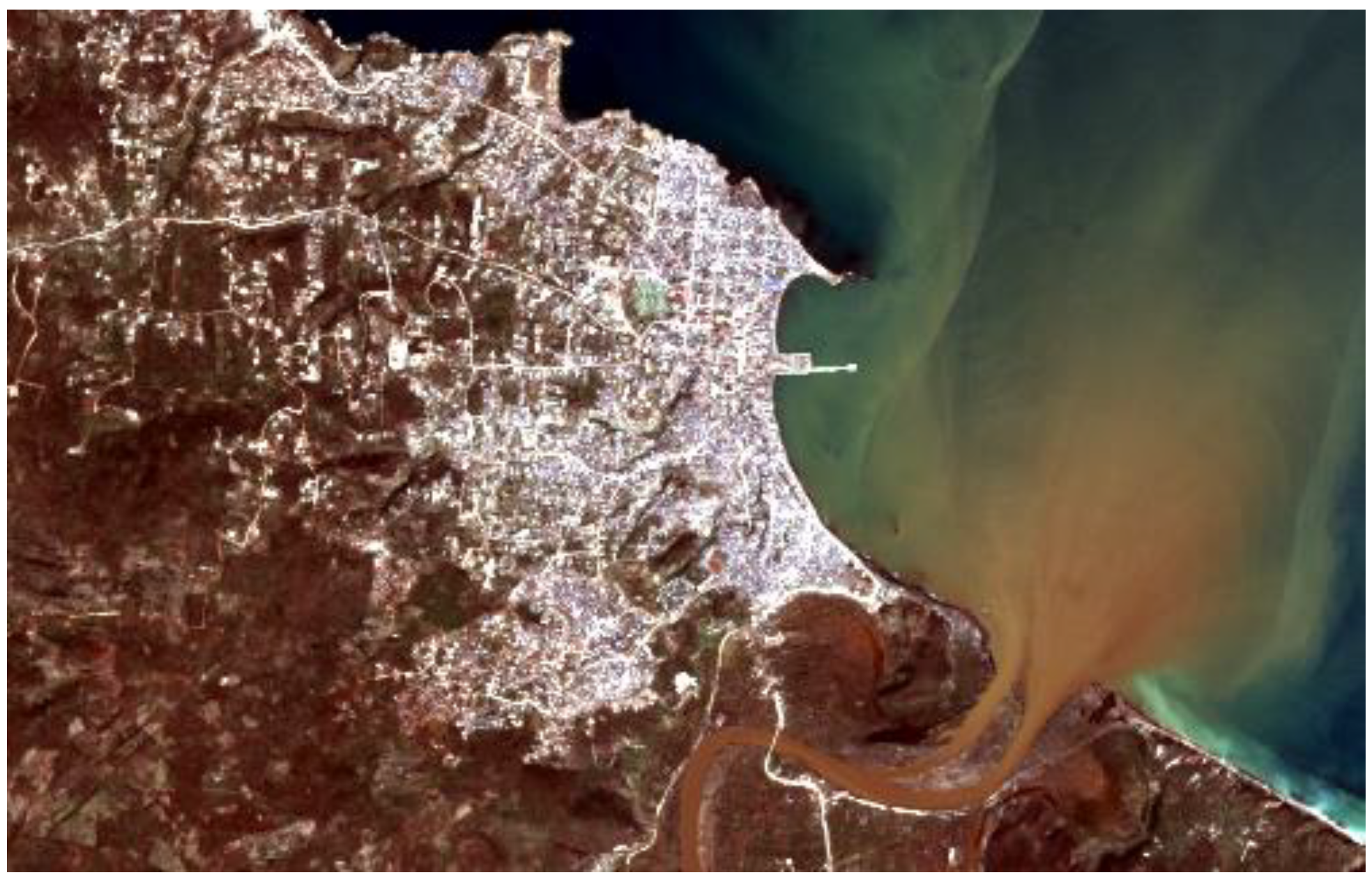
Figure 1. “Jérémie 2016” dataset: RGB true-color composition of the pansharpened multispectral Pléiades acquisition (image © CNES 2016, distribution Airbus DS).
Remotesensing 13 03509 g001
Figure 2. “Jérémie 2017” dataset: (a) RGB true-color composition of the multispectral Pléiades acquisition (image © CNES 2017, distribution Airbus DS); (b) Enhanced Spotlight SAR acquisition (COSMO-SkyMed Product © ASI—Italian Space Agency—2017. All rights reserved.).
Remotesensing 13 03509 g002
Figure 3. “Jérémie 2018” dataset: (a) RGB true-color composition of the multispectral Pléiades acquisition (image © CNES 2018, distribution Airbus DS); (b) StripMap HIMAGE SAR acquisition (COSMO-SkyMed Product © ASI—Italian Space Agency—2018. All rights reserved.).
Remotesensing 13 03509 g003
Figure 4. “Jérémie 2019” dataset: (a) RGB true-color composition of the multispectral Pléiades acquisition (image © CNES 2019, distribution Airbus DS); (b) Enhanced Spotlight SAR acquisition (COSMO-SkyMed Product © ASI—Italian Space Agency—2019. All rights reserved.).
Remotesensing 13 03509 g004
Figure 5. Block diagram of the proposed method. The products are the two classification maps corresponding to the two acquisition dates ( t 0 and t 1 ) and the change map identifying changes and specifying the transitions between land covers occurring between t 0 and t 1 .
Remotesensing 13 03509 g005
Figure 6. Graphical representation of the two different local neighborhoods used within the proposed energy function: (a) local neighborhood corresponding to the notation i j ; (b) local neighborhood corresponding to the notation i j .
Remotesensing 13 03509 g006
Figure 7. Experimental results obtained on the “Jérémie 2016” and “Jérémie 2017” datasets: (a) classification map corresponding to 2016; (b) classification map corresponding to 2017; (c) change map specifying the changes occurring between 2016 and 2017; (d) legend representing the class transitions in the change map. For the legend of the classification maps, we refer to Table 1.
Remotesensing 13 03509 g007
Figure 8. Classification maps obtained on the “Jérémie 2017”, “Jérémie 2018”, and “Jérémie 2019” datasets: (a) classification map corresponding to 2018; (b) classification map corresponding to 2019. For the legend of the thematic maps, we refer to Table 2. Black pixels indicate unclassified areas where no data were available (e.g., cloud masking or out of the satellite footprint).
Remotesensing 13 03509 g008
Figure 9. Change maps obtained on the “Jérémie 2017”, “Jérémie 2018”, and “Jérémie 2019” datasets: (a) change map specifying the changes that happened between 2017 and 2018; (b) change map specifying the changes that happened between 2018 and 2019; (c) legend representing the class transitions in the change maps.
Remotesensing 13 03509 g009
Figure 10. Details of the 2016 and 2017 datasets: (a) RGB composition of the optical image acquired in 2016; (b) RGB composition of the optical image acquired in 2017 (image © CNES 2016–2017, distribution Airbus DS); (c) grey-level representation of the SAR image acquired in 2017 (COSMO-SkyMed Product © ASI—Italian Space Agency—2017. All rights reserved.); (d) classification map corresponding to 2016; (e) classification map corresponding to 2017; (f) change map specifying the changes that happened between 2016 and 2017. The legend of the change map is displayed in Figure 11, while the legend of the classification maps is provided in Table 3.
Remotesensing 13 03509 g010
Figure 11. Legend representing the class transitions in the change map of Figure 10f.
Remotesensing 13 03509 g011
Figure 12. Details of the mouth of the Grande Anse River: (a) RGB composition of the optical image acquired in 2016 with the indication of the considered crop; (b) RGB composition of the optical crop acquired in 2016; (c) RGB composition of the optical crop acquired in 2017 (image © CNES 2016–2017, distribution Airbus DS); (d) classification map corresponding to the crop of 2016; (e) classification map corresponding to the crop of 2017; (f) change map corresponding to the timeframe 2016–2017; (g) legend of the change map. The legend of the classification maps is given in Table 1.
Remotesensing 13 03509 g012
Figure 13. (a) The 2019 classification map (see Figure 8 and related legend) with indication of (b) the bare-soil land cover transition at the mouth of the Grande Anse River and along the coast, south of Jérémie. Black dots mark the GPS locations of the ground-truth photographs showing (c) the sand and gravel river mouth bar interspersed with widespread rubbish and waste and (d) mining and quarrying activity occurring on-site in April 2019.
Remotesensing 13 03509 g013
Figure 14. Details of the southwestern “urban/anthropogenic” sector of Jérémie: (a) RGB composition of the optical image acquired in 2018 with the indication of the considered crop; (b) RGB composition of the optical crop acquired in 2017; (c) RGB composition of the optical crop acquired in 2018 (image © CNES 2017–2018, distribution Airbus DS); (d) classification map corresponding to the crop of 2017; (e) classification map corresponding to the crop of 2018; (f) change map corresponding to the timeframe 2017–2018. The legend of the change map is given in Figure 9, while the legend of the classification maps is provided in Table 1.
Remotesensing 13 03509 g014
Figure 15. Results obtained with and without SAR data: (a) RGB composition of an optical crop acquired in 2016 (image © CNES 2017–2018, distribution Airbus DS); (b) RGB composition of an optical crop acquired in 2017 (image © CNES 2017–2018, distribution Airbus DS); (c) change map obtained without using the COSMO-SkyMed data and corresponding to the timeframe 2016–2017; (d) change map obtained using the COSMO-SkyMed data and corresponding to the timeframe 2016–2017. The legend is the one provided in Figure 10c.
Remotesensing 13 03509 g015
Figure 16. Right bank of the Grande Anse River, south of Jérémie: classification maps corresponding to (a) 2017, (b) 2018, and (c) 2019 (see Figure 7 and Figure 8 and related legend), with indication of (d) dirt road leading to rural shacks and (e) unregulated and uncontrolled dump site, interspersed with (f) low vegetation and bush and where (g) garbage and plastic waste are also burnt.
Remotesensing 13 03509 g016
Figure 17. Cohen’s κ of the classification maps with respect to the test samples as a function of the number of scales Q used in the Markovian fusion framework.
Remotesensing 13 03509 g017
Figure 18. Different initializations in the case of Jérémie 2016: (a) initial classification map obtained via the method in [78]; (b) initial classification map obtained via RF; (c) final classification map obtained with the initialization in (a); (d) final classification map obtained with the initialization in (b). The legend is given in Table 1.
Remotesensing 13 03509 g018
Table 1. Accuracy scores for the two classification maps obtained with the datasets “Jérémie 2016” and “Jérémie 2017”. The corresponding maps are shown in Figure 7a,b. Legend: OA = overall accuracy, AA = average accuracy, PA = producer accuracy, UA = user accuracy, kappa = Cohen’s 𝜅 statistic.
Jérémie 2016Jérémie 2017
ClassPAUAClassPAUA
Water100%100% Water97.3%100%
Urban/Anthropogenic100%100% Urban/Anthropogenic100%97.4%
Tall Veg.99.2%95.3% Tall Veg.100%100%
Low Veg.95.1%99.2% Low Veg.97.0%100%
Muddy Water100%100% Bare soil100%89.1%
OA98.9%OA98.9%
AA98.9%AA98.9%
kappa98.6%kappa98.8%
Table 2. Accuracy scores on the test samples for the classification maps corresponding to the datasets “Jérémie 2018” and “Jérémie 2019” and obtained with the 2017–2018 and 2018–2019 temporal pairs, respectively. The corresponding maps are shown in Figure 8a,b.
ClassJérémie 2018Jérémie 2019
PAUAPAUA
Water100%100%100%100%
Urban/Anthropogenic98.4%100%98.4%100%
Tall Veg.99.4%100%100%100%
Low Veg.100%98.0%100%98.5%
Bare Soil100%100%100%100%
OA99.5%99.6%
AA99.6%99.7%
kappa99.3%99.5%
Table 3. Accuracy scores on the test samples for the two classification maps obtained with the datasets “Jérémie 2016” and “Jérémie 2017” at the resolution of 2 m and using 4 segmentation maps. The corresponding maps are shown in Figure 10d,e.
Zoom Jérémie 2016Zoom Jérémie 2017
ClassPAUAClassPAUA
Urban/Anthropogenic100%100% Urban/Anthropogenic98.6%100%
Shrubs and bush100%100% Shrubs and bush100%97.5%
Grass100%100% Grass95.6%100%
OA100%OA98.9%
AA100%AA98.1%
kappa100%kappa98.1%
Publisher’s Note: MDPI stays neutral with regard to jurisdictional claims in published maps and institutional affiliations.