Article

Multidimensional Assessment of Food Provisioning Ecosystem Services Using Remote Sensing and Agricultural Statistics

1
College of Surveying and Geo-Informatics, Tongji University, Shanghai 200092, China
2
Department of Geography, University of Tennessee, Knoxville, TN 37996, USA
3
Urban Surveyors, Shanghai 200003, China
*
Author to whom correspondence should be addressed.
Remote Sens. 2020, 12(23), 3955; https://doi.org/10.3390/rs12233955
Submission received: 3 November 2020 / Revised: 27 November 2020 / Accepted: 30 November 2020 / Published: 3 December 2020

Abstract

:
With the increasing global population, human demands for natural resources continue to grow. There is a critical need for the sustainable use and development of natural resources. In this context, ecosystem services have attracted more and more attention, and ecosystem services assessment has proven to be useful for guiding research, policy formulation, and management implementation. In this paper, we attempted to assess ecosystem services more comprehensively from various perspectives. We used food provisioning ecosystem services in Minnesota as a case study and proposed two new concepts for assessing ecosystem services: efficiency and trend. We designed a multidimensional assessment framework, analyzed the total output, efficiency, and trend temporally based on both area and space with Exploratory Spatial Data Analysis (ESDA). We also identified major influencing factors based on remote sensing images in Google Earth Engine and explored the quantitative influence on each assessment dimension. We found that: (1) Food provisioning ecosystem service in Minnesota has generally been improving from 1998 to 2018. (2) We identified food provisioning ecosystem services in Minnesota as superior zones, mixed zones, and inferior zones with a ‘sandwich geo-configuration’. (3) The total output tends to be stable while the efficiency is disturbed by some natural disasters. Simultaneously, the trend index has been improving with slight fluctuations. (4) Agricultural disaster financial support has a stronger impact on stabilizing the total output of food provisioning than the other two dimensions. (5) Soil moisture, diurnal temperature difference, and crop growth are the three main influencing aspects of food provisioning ecosystem services, and the order of the influential density is: the Perpendicular Drought Index (PDI), Normalized Difference Vegetation Index (NDVI), Rainfall (RF), Daytime Temperature (DT), and Diurnal Temperature Difference (DIF).

Graphical Abstract

1. Introduction

Ecosystem services are the various benefits provided to humans by the natural environment. With the increasing global population, human demands for natural resources continue to grow. There is a critical need for the sustainable use and development of natural resources. Various definitions of ecosystem services have been proposed in the literature. For example, Costanza et al. [1] defined ecosystem services as natures direct or indirect contribution to human welfare and classified them into 17 categories. Daily et al. [2] proposed that ecosystem services are the conditions and processes through which natural ecosystems, and the species that make them up, sustain and fulfill human life. The Millennium Ecosystem Assessment (MA) defined ecosystem services as all the benefits humans obtain from the ecosystems, including provisioning services (e.g., food and water), regulating services (e.g., flood controlling and disease controlling), cultural services (e.g., spiritual, entertainment and cultural gains) and supporting services (e.g., the nutrient cycle that maintains the living environment on Earth) [3,4]. In this paper, we proposed a new framework for multidimensional assessment of food provisioning ecosystem services.
There have been three popular methods for ecosystem services assessment proposed in the literature, namely the monetary assessment methods, energy-based methods, and material-based methods. Ecosystem monetization attempts to assign monetary values to nature’s services [5], which offers a framework that can be easily understood by a wide audience, making it a useful decision-making tool for government finance. It is an attractive option for policymakers and public officials who are facing time and budget constraints [6]. Therefore, various economic methods have been developed to assess the economic value of ecosystem services. For example, Ratisurakarn [7] estimated the economic value of forest ecosystem services by adopting a meta-analysis. Davis [8] groundbreakingly applied a contingent valuation method to evaluate goods or services with consumers’ payment willingness in a hypothetical market. Other noteworthy monetary assessment methods include: the market value method (using the output value variations of a certain area caused by natural environment changes as the economic effect of environmental alteration) [9], the shadow pricing method (using the cost of artificially projects to replace the original environmental function as the economic loss of polluted or destroyed environmental parts) [10], and the value transfer method (grafting the ecosystem economic value per unit area in the existing research to the study area) [11,12,13]. These methods have made a significant contribution to the economic value assessment of ecosystem services. The concepts, application scope, calculation methods of these methods have been further explored based on their various characteristics and applicabilities [14,15,16,17].
However, the monetary assessment methods have some limitations: (1) it is vital to choose a proper method to match the research targets and goals since the results of different methods vary greatly; (2) economic methods do not fit ecosystems perfectly since ecosystem services are not actual market behaviors and, with the circumstance updating, the changing human demand has required different assessments; (3) the dependence derived from the complexity of the ecosystem itself caused double counting or undercounting in the economic results [18]. The other two mainstream methods (i.e., energy-based and material-based methods) arose from the demand for more objective assessments evoked by the uncertainty, instability, even some errors in economic methods. Energy-based methods measure ecosystem services with the amount of solar energy the ecosystem absorbed, the ecosystem conversion or material output [19,20,21,22,23,24]. Material-based methods use the amount of ecosystem service carriers exported to human beings to measure ecosystem services, for example, the weight of food that humans obtain from an ecosystem reflects the amount of food provisioning ecosystem services [25]. In recent years, based on these methods and theories, ecosystem services evaluation models supported by remote sensing data, socioeconomic data, and geospatial technologies have become one of the most focal areas, such as the Integrated Valuation of Ecosystem Services and Trade-offs (InVEST), Carnegie-Ames-Stanford Approach (CASA), Social Values for Ecosystem Services (SoLVES), and Artificial Intelligence for Ecosystem Services (ARIES) [26,27,28,29,30,31,32,33,34]. As a carrier of food provisioning ecosystem services, the food humans obtain directly from nature has abundant weight statistics and good accessibility. Thus, we adopted the material-based method in this paper.
Ecosystem services assessment has made great progress in data, technologies, methods, and scales. However, there are some limitations to existing studies: (1) Economic methods, energy-based methods, and material-based methods focus on ecosystem services output or storage [1,12,35,36,37]. However, few studies explored the efficiency or trend of ecosystem services. (2) Existing studies rarely explored the influencing factors on ecosystem services [4,13,38], let alone analyzing their quantitative relationships. (3) Most ecosystem service assessments did not reach the full potential of remote sensing. Traditional approaches are usually based on statistics and vector data. Since the rise of the model methods, remote sensing images have been mostly used for identifying land cover [24,29,30,39,40,41,42,43] and have rarely been used in exploring the influencing factors of ecosystem services. However, various remote sensing products and indices are quantitatively related to some ecosystem services [44,45,46,47,48,49,50,51,52], such as biomass, crop yield, water quality, and biological habitat.
This study aimed to assess food provisioning ecosystem services comprehensively from various perspectives, building a framework in which the output, efficiency, and trend could be reflected simultaneously. Based on the theory of material quality evaluation, we believe that the amount of harvested crops can reflect the food provisioning ecosystem services. Compared with previous studies, the highlights of this paper are as follows: (1) We proposed two new concepts in ecosystem services assessment. One is the ecosystem service efficiency, which is the output of a unit ecosystem area, reflecting the quality of the ecosystem. The other is the ecosystem trend, reflecting the trend of ecosystem efficiency. The trend index is a vector whose direction and magnitude represent the trend and rate of change, respectively. (2) We designed an assessment framework to evaluate ecosystem services from three different aspects: total output, efficiency, and trend. (3) We analyzed the temporal changes of each dimension from the perspectives of area and geographic patterns. (4) We identified the main influencing aspects and analyzed the quantitative relationship between remote sensing indices and each assessment dimension using the Google Earth Engine cloud computing platform.

2. Materials and Methods

2.1. Study Area

We chose the state of Minnesota (Figure 1) as our study area. Minnesota is the 12th largest in area, the 22nd most populous [53], and the 5th largest in agricultural production among all U.S. states [54]. Agriculture is the second largest industry in Minnesota, accounting for USD 57.5 billion in sales and more than 147,000 jobs [54].
Minnesota consists of 87 counties, covering 225,163 square kilometers. Given that the data of agricultural statistics are county-based, we performed the analysis at the county level.

2.2. Data Sources

We used statistical data from the U.S. Department of Agriculture (USDA) [55] to calculate multidimensional assessment indicators at the county level. Remote sensing images from the Google Earth Engine data catalog [56,57,58] were used to extract influencing factors. We selected corn, wheat, oat, and soybean as the main crops in Minnesota according to the Minnesota State Agriculture Overview [59].

2.3. Methods

We designed a multidimensional assessment framework and applied it to the 87 counties. Exploratory Spatial Data Analysis (ESDA) was adopted to explore the geospatial pattern of the results. We extracted remote sensing indices via Google Earth Engine and analyzed their quantitative relationships with the multidimensional assessment results. There were some statistical analysis methods used in this paper. The following sections describe the main methods we used.

2.3.1. A Multidimensional Assessment Framework

We proposed a multidimensional assessment framework (Figure 2) that uses the total output (P), efficiency (Q), and trend (D) to uniquely characterize ecosystem services. It defines eight assessment spaces as shown in Table 1.
In Figure 2b, objects ‘a’ and ‘d’ are located in Space V, ‘b’ is located in Space III, and ‘c’ is located in Space II. That is to say, ‘a’ and ‘d’ share the properties of Space V, and ‘b’ and ‘c’ share the properties of Space III and Space II, respectively. However, ‘a’ has stronger properties compared to ‘d’ because it has a larger assessment cuboid.
The food humans obtain from nature mainly depends on the agriculture sector. Crop production is a branch of agriculture dealing with growing crops for use as food and fiber [60]. It is an effective indicator reflecting the total amount of food provisioning ecosystem services. Thus, the P-score in our research was derived from the main crop production. We defined ecosystem service efficiency as the ecosystem service output of a unit area, so the crop yield reflects the food provisioning ecosystem service efficiency. D-score is the trend index of food provisioning ecosystem service, calculated by the annual change in efficiency.
Due to the different value ranges of multi-source datasets used in this study, we standardized the data, i.e., rescaling the data to have a mean of 0 and a standard deviation of 1. This standardization is called a z-score, which can reflect the gap between data points and the overall average. A z-score can be calculated with the following formula:
x * = x x ¯ σ
where x *   is the z-score, x ¯ is the mean of the original data, σ is the standard deviation of the original data. Above-average data points will get a positive z-score, while subaverage data will get a negative z-score. The absolute value of the score indicates the number of standard deviations between the data points and the average. We used this z-score standardization method to calculate the P, D, and Q scores, which reflect the total output, efficiency, and trend of the food provisioning ecosystem services relative to the average level, respectively (Table 2).
The multidimensional assessment framework has the following characteristics:
  • It is a relative assessment framework based on the average level. P-score, Q-score, and D-score are normalized to (−3,3). A positive index means an above-average dimension; the larger the index, the better the circumstance. Conversely, a negative index indicates a subaverage dimension; the lower the index is, the worse the circumstance is.
  • P-score, Q-score, and D-score uniquely determine the characteristics of each county. The volume of the assessment cuboid reflects the strength of the characteristics it shows.

2.3.2. Exploratory Spatial Data Analysis

Initially, Tukey [61] proposed a new method of exploratory data analysis (EDA) to solve the problems in traditional statistics: (1) The practical data cannot meet the normal assumption. (2) The models based on mean and variance tend to have low stability. EDA was able to analyze massive data, made no assumption of the population, and often excluded hypothesis testing. It tried to ‘let the data speak’ via statistical charts, graphs, and statistical overview methods. Exploratory Spatial Data Analysis (ESDA) is the expansion of EDA in the field of spatial data analysis. ESDA is supported by spatial analysis, emphasizes the spatial correlations of events, and focuses on the nature of spatial data. It is a powerful tool for geospatial data analysis, such as exploring spatial patterns, extracting main characteristics, identifying spatial clusters, evaluating aggregated and discrete patterns, grouping objects, and modeling spatial relationships. We adopted ESDA to explore the geographic spatial distribution and clustering patterns of food provisioning ecosystem services in Minnesota.
Hot-Spot Analysis, one of the main methods of ESDA, is based on the Getis-OrdGi* algorithm Equation (2) proposed by J. Keith Ord and Arthur Getis [62]. It focuses on identifying geospatial clusters of statistically high values (hot spots) and low values (cold spots). In a ‘hot spots’ zone, the high value is surrounded by high value. Similarly, a low value is located at the low-value gathering area in ‘cold spots’ zone.
G i * = j = 1 n w i j x j x ¯ j = 1 n w i j j = 1 n x j 2 n 1 x 2 [ n j = 1 n w i j w ( j = 1 n w i j ) 2 ] n 1
where G i * is positive for a ‘hot spot’ and negative for a ‘cold spot’. The statistical significance is assessed by Z test in which the z-score and p-value are statistical significance measures and the accordances of whether to reject the null hypothesis or not (Table 3). In fact, they determine whether the observed spatial clusters are more obvious than we expected in a random distribution.

2.3.3. Remote Sensing Image Analysis

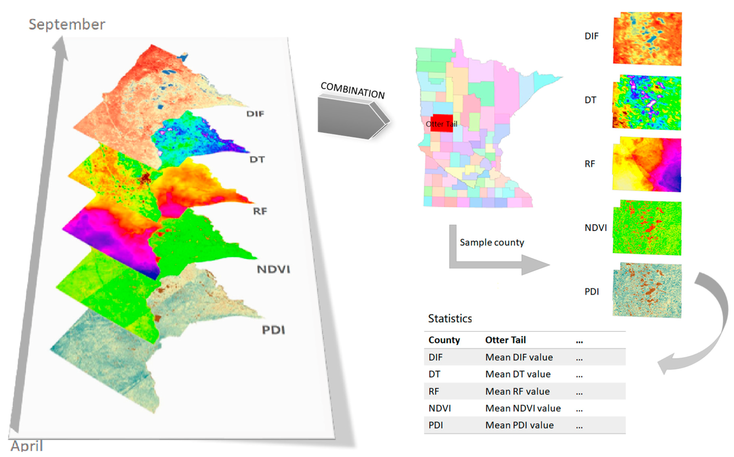
The modeling results, based on remote sensing data, could be very different from current conditions. Given that 2018 is the closest time period to the present, we believe that 2018 is more meaningful for recent policy-making and ecosystem management than other time periods (i.e., 1998, 2003, 2008, 2013). Therefore, we selected 2018 as a case in modeling the influencing factors of food provisioning ecosystem services. We used remote sensing images acquired in 2018 to extract the influencing factors of the multidimensional assessment results. The typical crop growing season in Minnesota ranges from May to September [63,64,65]. To supplement some unusable satellite images acquired in May due to high cloud coverage, we extended the time range from April to September. Vegetation conditions and climatic conditions are the key factors affecting crop yield [45,47,66]. We chose the Perpendicular Drought Index (PDI) [47], Normalized Difference Vegetation Index (NDVI), Rainfall (RF), Daytime Temperature (DT), and Diurnal Temperature Difference (DIF) as the main influencing factor indicators (Figure 3).
We derived the five influencing factors from remote sensing images at the pixel scale and then aggregated them to the county level. We used various remote sensing images in this paper and combined remote sensing data with vector data, resampling the pixels of remote sensing images from a micro perspective to a wider range of county boundaries to avoid the problems of different temporal and spatial resolutions of various remote sensing images.
We used the USGS Landsat 8 Surface Reflectance Tier 1 (30-m resolution) data, which have been atmospherically corrected, to calculate the PDI and NDVI. The formulas are as follows:
P D I = ( R r e d + M × R n i r ) / ( M 2 + 1 )
N D V I = ( R n i r R r e d ) / ( R n i r + R r e d )
where R r e d and R n i r are the red band and near-infrared band of Landsat images, respectively. M is the slope of the soil line (Formula (5)), β is a constant.
R n i r = M × R r e d + β
DT and DIF data are from the dataset MOD11A2 Terra Land Surface Temperature and Emissivity 8-Day Global, which provides an average 8-day land surface temperature (LST). Daily Surface Weather and Climatological Summaries provide the RF data. These datasets are readily available in the Earth Engine public data catalog.

2.3.4. Statistical Analysis

(1) Principal Component Analysis
Principal component analysis (PCA) is one of the most widely used statistical methods for dimensionality reduction. It was first introduced by K. Pearson [67]. It is the process of computing the principal components and using them to perform a change of basis on the data, sometimes using only the first few principal components and ignoring the rest [68]. We used the five influencing factors as the original dataset and extracted their principal components.
(2) Multiple Linear Regression
Multiple linear regression attempts to model the relationship between two or more explanatory variables x i and a response variable y i by fitting a linear equation to observed data. The model for multiple linear regression, given N observations, is:
y i =   β 0 + β i x i + ε i ,   i = 1 , 2 , 3 , , N
In the least-squares model, the best-fitting line for the observed data is calculated by minimizing the sum of the squares of the vertical deviations from each data point to the line (if a point lies on the fitted line exactly, then its vertical deviation is 0). The restriction formula is:
Q ( β 0 ,   β 1 , β 2 ,   ,   β p ) = i = 1 N ( y i y ^ i ) 2 = i = 1 N ( y i β 0   β 1 x i 1 β 2 x i 2 β p x i p ) 2   M I N
In this paper, x i indicates the five influencing factors; y i represents the multidimensional assessment indicators; the values fitted by Equation (6) are donated y ^ i .

3. Results

3.1. Multidimensional Assessment Area Results

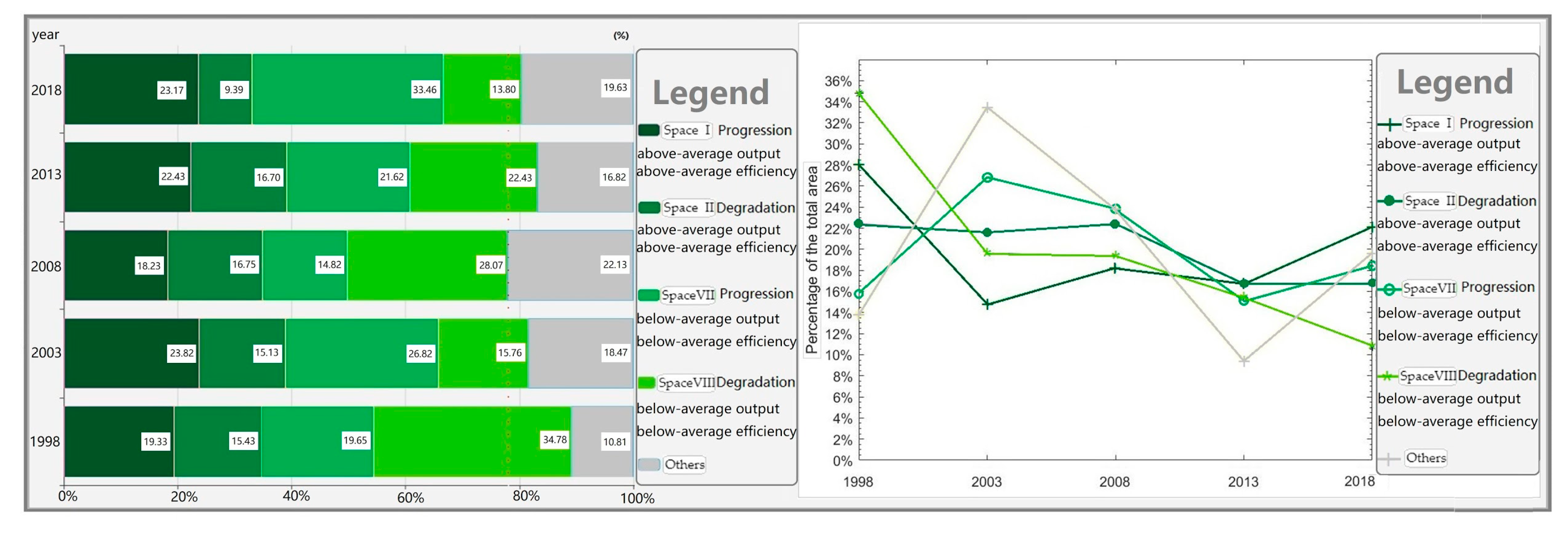
As shown in Figure 4, there are four dominant spaces in Minnesota (see Figure 2 for the eight spaces), including: progression zones with above-average output and efficiency (Space I), degradation zones with above-average output and efficiency (Space II), progression zones with below-average output and efficiency (Space VII), and degradation zones with below-average output and efficiency (Space VIII). These four dominant spaces accounted for more than 77% of the total area. Thus, our subsequent analysis focused on these four spaces (i.e., I, II, VII, and VIII).
Their developments are as follows: (1) Degradation zones with subaverage output and efficiency (Space VIII) dropped significantly, from 34.78% in 1998 to 10.81% in 2018. (2) The trend of progression zones with below-average output and efficiency (Space VII) turned over from 2003 to 2013. It rose before 2003, then began to decline, resumed an upward trend after 2013 (Figure 4). (3) Progression zones with above-average output and efficiency (Space I) decreased to 14.82% from 28.07% in the first period (1998–2003), but it has risen steadily since 2003 and reached 22.13% in 2018. (4) Degradation zones with above-average output and efficiency (Space II).
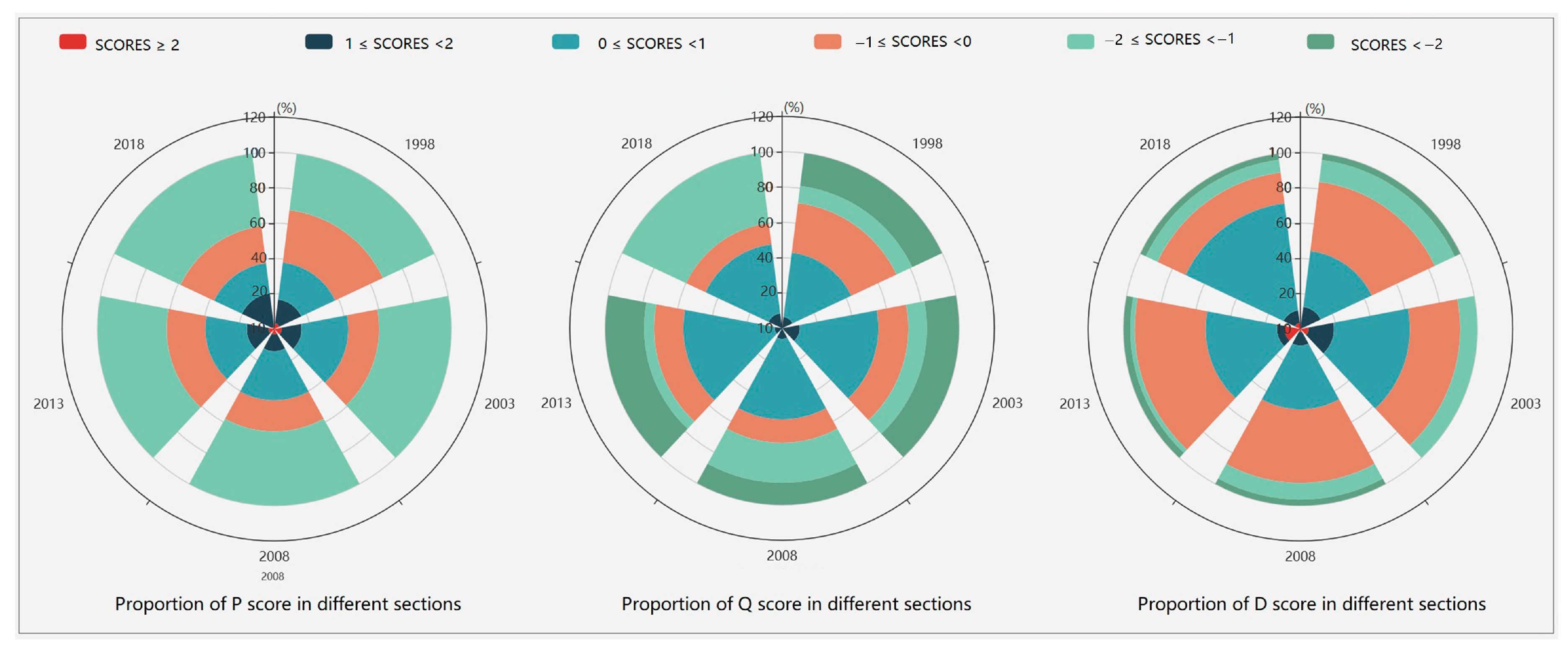
The value of score indicates the level of research target compared to the average. A positive score means an above-average level and a negative score indicates a below-average level. We divided the results into six categories with an equal interval: (1) Scores greater than 2, indicating they are more than twice the standard deviation above the average level. (2) Scores in [1, 2) are one to two times of standard deviation above the average level. (3) Scores in [0, 1) are within one standard deviation above the average level. (4) Scores in [−1, 0) are within one standard deviation below the average level. (5) Scores in [−2, −1) are one to two standard deviations below the average level. (6) Scores less than −2 are more than twice the standard deviation below the average level.
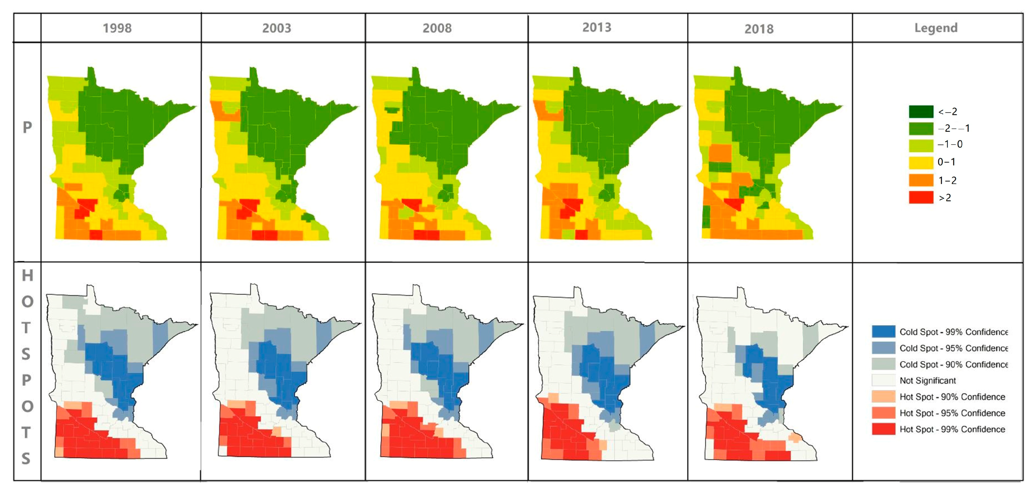
P-score in Minnesota is mainly in (−2, 1), accounting for more than 80% of the total area, in which the negative P-score zones account for around 60%. It shows in 80% of the area in Minnesota that the output ranges from two standard deviations below average to one standard deviation above average, and the below-average part is dominating. Figure 5 shows that the area pattern of the P-score has been stable from 1998 to 2018. The negative P-score area has always been larger than the positive, indicating that the below-average output area has been larger than the above-average output area.
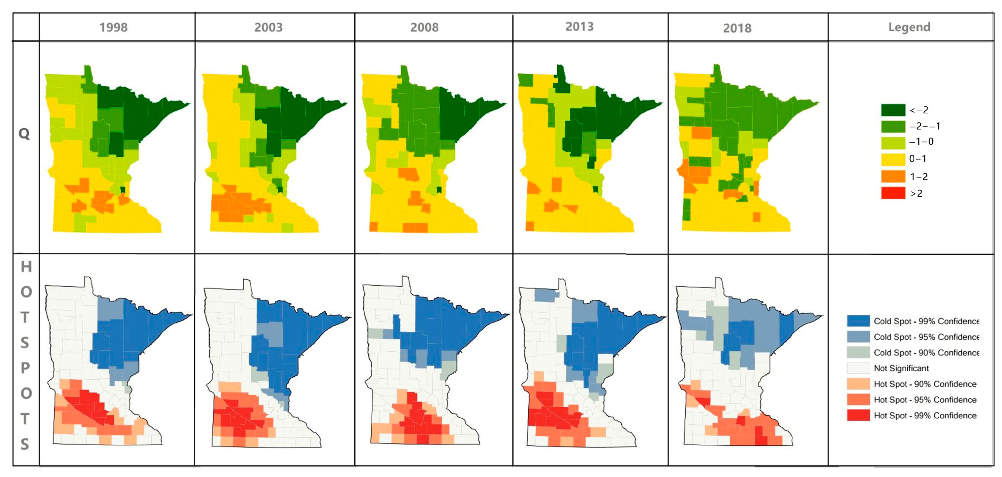
Similar to the P-score, more than 70% of the area in Minnesota has a Q-score within (−2, 1). That is to say, in 70% of the area, the food provisioning ecosystem service efficiency is from two standard deviations below average to one standard deviation above average, and this section increased to 91% in 2018. The above-average efficiency area (positive Q-score) is similar to the below-average efficiency area (negative Q-score) and the largest section is one standard deviation above-average area (0 < Q-score < 1), accounting for around 40% of the total (Figure 5).
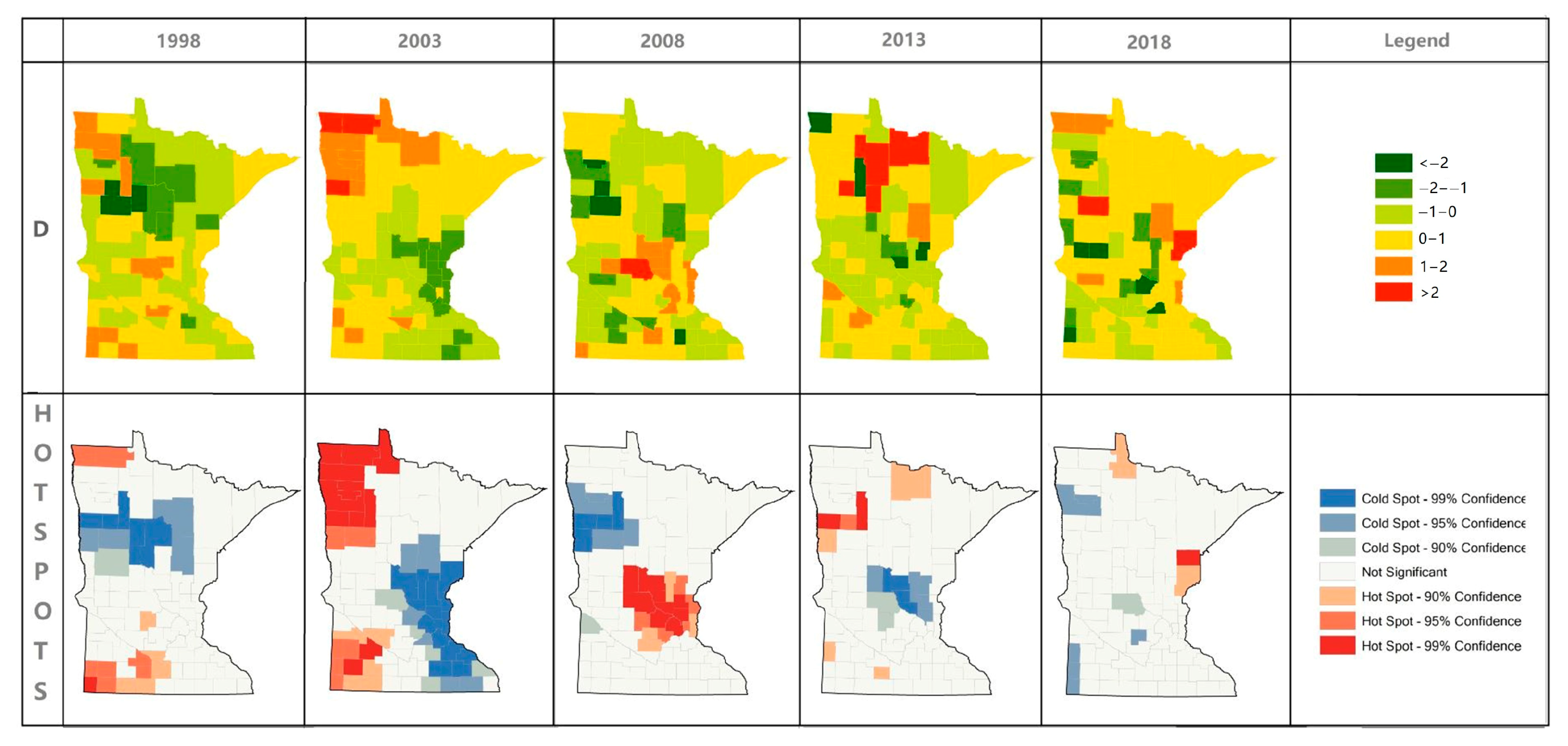
More than 70% of the area had a D-score between (−1, 1), indicating that the trend index was very close to the average level. Figure 5 shows that the above-average trend index area (positive D-score), the progression area, gradually overtook the below-average part (negative D-score), the degradation area. Thus, it is reasonable to believe that the food provisioning trend in Minnesota has improved. The areas of (1, 2) and (−2, −1) were gradually shrinking, which means more and more areas have been approaching the average trend level. In other words, the regional gap in the trend index has been decreasing.

3.2. Multidimensional Assessment Geography Spatial Results

The multidimensional assessment results were analyzed based on the nine agricultural districts as defined by the United States Department of Agriculture (USDA) (Table 4):

3.2.1. Multidimensional Assessment of Spatial Analysis

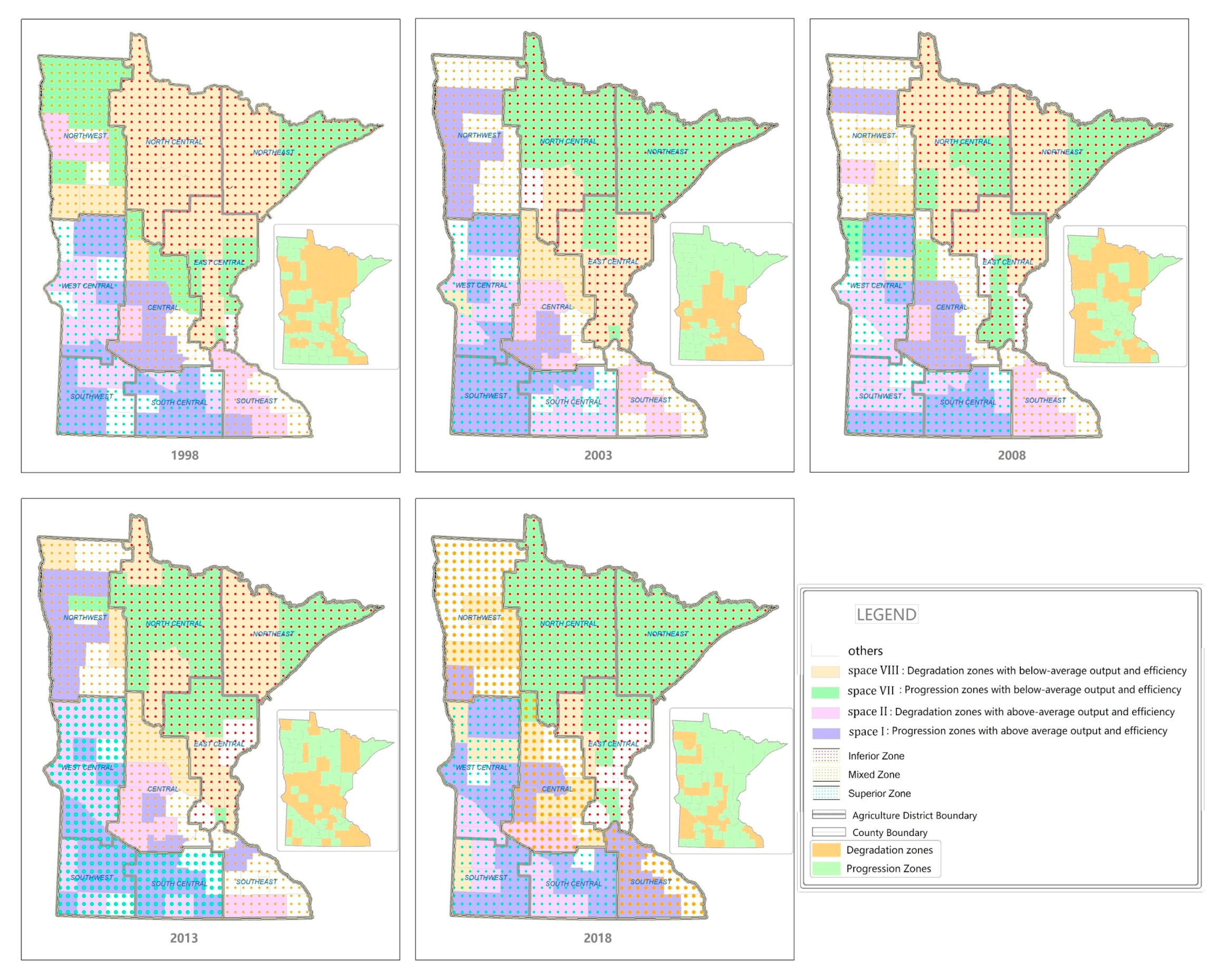
We identified Minnesota in the inferior zones, mixed zones, and inferior zones according to the distribution of assessment spaces and found that they located as a ‘sandwich geo-configuration’ pattern. The superior zones were covered by progression zones with below-average output and efficiency (Space VII) and degradation zones with below-average output and efficiency (Space VIII), including North Central, Northeast, and East Central. The superior zones were dominated by progression zones with above-average output and efficiency (Space I) and degradation zones with above-average output and efficiency (Space II), spreading over West Central, Southwest, and South Central. The others were identified as mixed zones since they were mixed by the inferior zones and the superior ones.
Figure 6 shows that the inferior zones and superior zones have stable temporal and spatial distribution but the mixed zones have changed a lot.

3.2.2. Total Output Geospatial Analysis

A ‘sandwich geo-configuration’ located in P-score distribution and in the geospatial cluster (Figure 7): The inferior zones covered by the much below average P-score, [−3, −1), with the cold spots. The hot spots are located in the superior zones with the much above average P-score, [1, 3]. The mixed zones did not have significant clusters and they were dominated by the around average P-score, [−1, 1).

3.2.3. Efficiency Geospatial Analysis

The distributions of Q-score did not follow the ‘sandwich geo-configuration’ (Figure 8). The much below average Q-score was located in the inferior zones, while others were randomly spread over the superior zones and the mixed zones. However, the geospatial cluster in Q-score was similar to the P-score; cold spots were in the inferior zones, and hot spots were located in the superior zones. The hot spots were transferred to the southeast from the southwest.

3.2.4. Trend Geospatial Analysis

The D score does not have a stable spatial distribution pattern, and it changes frequently from 1998 to 2018 (Figure 9). The hot spot analysis results showed that the geospatial cluster in Minnesota disappeared gradually, indicating that the trend index was geospatially randomized.

3.3. Influencing Factors Analysis

3.3.1. Principal Component Analysis of Influencing Factors

Based on existing studies [45,46,47] and the data availability, five indicators were selected in this paper, including the Perpendicular Drought Index (PDI), Normalized Difference Vegetation Index (NDVI), Rainfall (RF), Daytime Temperature (DT), and Diurnal Temperature Difference (DIF). We used the average value of remote sensing images during the crop growing season (from May to September). The principal component analysis divided these variables into three comprehensive indices and the principal component loads are shown in Table 5.
The five factors influencing the food provisioning ecosystem service are classified into three types, i.e., soil moisture, diurnal temperature difference, and crop growth. It can be seen from Table 5 that the first principal component Z 1 has a large positive correlation with the variables related to soil moisture, the PDI, RF, and DT. Thus, the first principal component is regarded as a representative of soil moisture. The second principal component Z 2 has a large positive correlation with DNT, which is related to the temperature difference between day and night, so the second principal component is regarded as a representative of the day and night temperature difference. The third principal component Z 3 has a large positive correlation with NDVI, which is related to crop growth, so the third principal component is regarded as a representative of crop growth.

3.3.2. Multiple Linear Regression Analysis of Influencing Factors and Assessment Results

To explore the influence of each factor on different assessment dimensions, a multiple linear regression analysis based on assessment results was adopted:
P =   4.71 + 10.45 P D I 4.90 N D V I + 0.14 R F + 0.03 D T + 0.19 D N T
Q =   5.82 + 11.55 P D I 1.70 N D V I + 0.12 R F + 0.02 D T + 0.16 D N T
D + =   0.68   + 6.77 P D I 2.82 N D V I + 0.04 R F 0.01 D T + 0.03 D N T
D =   2.72 5.41 P D I 0.59 N D V I 0.06 R F 0.10 D T
Compared with the F-test critical value table, all the F-test scores (Table 6) we got are greater than the standard values at their corresponding confidence levels. Therefore, we believe that the linear regression calculation results are credible.
The positive and negative D-scores have different regression equations, indicating that there are different ways the influencing factors affect the degrading food provisioning ecosystem service and the evolving one.

4. Discussion

4.1. Multidimensional Assessment Results Discussion

Our results indicate that the food provisioning ecosystem service in Minnesota is significantly polarized, which is dominated by superior zones (Space I, Space II) and inferior zones (Space VII and Space VIII). The results also show that it has come a long way since the area of extra inferior zones (Space VIII) has shrunk considerably. While there is an exigent circumstance with degrading zones in Minnesota, which reached a portion of 50.21% in 2018. However, some improvements have been witnessed by the shrinking area of bad ecosystem service zones and the geospatially steady distributions of total output and efficiency, as well as the spatial homogenization of trend index.

4.2. Spatiotemporal Patterns of Multidimensional Assessment Results

The various dimensions have different development patterns. The P-score has developed steadily with a pretty good overall condition. It is witnessed by its range, (−2, 3), without extra-low value. However, the Q-score fluctuated sharply, especially in the last two five-year periods. The D-score has been always located in (−1,1), which means the trend index is relatively evenly distributed in the studied region. It is known that government agricultural disaster payments have irreplaceable positions in fighting weather extremes and ensuring food provisioning [69,70], whose distributions are affected by disastrous weather events. Thus, government agricultural disaster payments reflect the strength of agricultural disasters in the year. We noticed that the most agricultural disaster payments in Minnesota happened in the second period (2003–2008, 2008 is excluded), 303.48 million dollars, followed by the next five years, 199.60 million dollars [71]. Interestingly, the two sharp fluctuations in assessment results followed these two disaster periods, respectively. Thus, we believed that the disaster financial support stabilized the total output of food provisioning ecosystem service, but seemed unable to eliminate the impact on the efficiency and trend. This is consistent with the argument that agricultural disaster payments always subsidized market failure and focused on market returns [69]. At the same time, our findings bear a resemblance to the reasoning that subsidized disaster assistance and insurance may not prevent negative environmental effects from arising [72].
As the spatial patterns of multidimensional assessment results might be the consequences of ecological land distribution [73,74,75,76], it is reasonable that there is a significant boundary that separates Northeast, East Central, and North Central from the others in our results. This coordinates the reality that forests in Minnesota are mainly distributed in the northeast of the state, while cropland is mainly distributed in the southwest. The total output of food provisioning ecosystem service in Minnesota has steady temporally geospatial distribution and clustering patterns. However, there is a big difference between the amelioration in the northeast side of the state and the deterioration on the other side in ecosystem service efficiency. Its geospatial hotspot located in the south of the state has been moving toward the east, which is in line with the eastward population shifting in south Minnesota [77]. An obvious randomization in D-score reflects the spatially homogeneous development of food provisioning in the state of Minnesota.

4.3. Relationship between Multidimensional Assessment Results and Impacting Factors

Remote sensing vegetation indices (e.g., surface water indices, soil moisture, temperature condition, rainfall) have been proved to affect the crop yield [47,78,79]. In our research, we found that soil moisture, diurnal temperature difference, and crop growth are the three main influencing aspects of food provisioning ecosystem service. The influencing factors are ranked according to their strength as follows: PDI, NDVI, RF, DT, and DNT. It is worth noting that the negative coefficients of NDVI in the linear equations are the reflections of the extremely high NDVI of the forest zones with the weaker food provisioning ecosystem service, which is consistent with the results of Prasad’s study of Iowa [47].

4.4. Limitations and Future Research Direction

Our analysis constituted the first step in multiperspective assessment in ecosystem services evaluation. Nevertheless, there are some limitations in our research: (1) We took food provisioning as the case study, and subsequent research could address other ecosystem services. (2) Referring to the existing studies [45,46,47], we only chose five remote sensing indicators as the influencing factors. More remote sensing products and indicators that may have an impact on food provisioning ecosystem services need to be further explored. (3) We adopted linear models to explore the relationship between impact factors and assessment results. With the rise of machine learning and artificial intelligence application in the field of ecosystem service evaluation [80,81,82,83,84], we may explore smarter multidimensional assessment models with higher precision in subsequent research. (4) We only selected remote sensing images acquired in the growing season in 2018 as a case to explore the ecosystem services influencing factors. Future research can further explore how the quantitative relationship varies according to the dates and seasons of remote sensing images.

5. Conclusions

Our multidimensional ecosystem services assessment framework evaluates the total output, efficiency, and trend of the ecosystem service simultaneously. It could identify the hidden and degrading ecosystems which are disguised by their good status quo as well as the low-quality ecosystems whose outputs are highly dependent on the area scales, thereby helping the environment management and sustainable development of the region. The serious polarization of food provisioning ecosystem service in Minnesota should be paid more attention, and relevant departments should take some targeted measures to reduce the area of Space VII and Space VIII. The degradation of some zones cannot be ignored either, some superior zones (Space II) are degrading, and a considerable area of inferior zones (Space VII) is getting worse. To ensure the sustainable development of food provisioning ecosystem services, these degradations must be slowed down. We analyzed the temporal development of every assessment dimension and found that the agricultural financial support only stabilized the total output of food provisioning and it worked a little on the efficiency and trend when facing natural disasters such as tornadoes and extreme weather. However, the determination of the quantitative influence relationships of the main influencing factors on each assessment dimension may help us think about how to fix the weak sides of ecosystem services.
To understand and assess the ecosystem services more comprehensively and explore their hidden aspects that are largely ignored, we tried to build a quantitative assessment framework for evaluating ecosystem services from multiple perspectives. We only selected food provisioning ecosystem service as a case in this paper. There is no doubt that more multidimensional assessment methods of other ecosystem services can be explored in future work.

Author Contributions

Conceptualization, Q.W. and D.S.; Methodology, Q.W. and D.S.; Software, Q.W. and D.S.; Validation, Q.W., D.S., Y.S., and R.F.; Formal analysis, Q.W.; Investigation, D.S.; Resources, D.S. and Q.W.; Data curation, D.S. and R.F.; Writing—original draft preparation, D.S.; Writing—review and editing, Q.W. and Y.S.; Visualization, D.S.; Supervision, Q.W.; Project administration, Q.W., Y.S.; Funding acquisition, Y.S. All authors have read and agreed to the published version of the manuscript.

Funding

This research was supported by the Technology Innovation Center for Land Spatial Eco-restoration in Metropolitan Area, MNR, Shanghai, 200003. We would also like to thank the China Scholarship Council for sponsoring D.S. to study at the University of Tennessee as a visiting scholar.

Conflicts of Interest

The authors declare no conflict of interest.

References

  1. Costanza, R.; d’Arge, R.; de Groot, R.; Farber, S.; Grasso, M.; Hannon, B.; Limburg, K.; Naeem, S.; O’Neill, R.V.; Paruelo, J.; et al. The value of the world’s ecosystem services and natural capital. Ecol. Econ. 1998, 25, 3–15. [Google Scholar] [CrossRef]
  2. Daily, G.C. Nature’s Services; Island Press: Washington, DC, USA, 1997; Volume 3. [Google Scholar]
  3. Reid, W.V. Millennium Ecosystem Assessment; World Resources Institute: Washington, DC, USA, 2005. [Google Scholar]
  4. Carpenter, S.R.; Mooney, H.A.; Agard, J.; Capistrano, D.; Defries, R.S.; Díaz, S.; Dietz, T.; Duraiappah, A.K.; Oteng-Yeboah, A.; Pereira, H.M.; et al. Science for managing ecosystem services: Beyond the Millennium Ecosystem Assessment. Proc. Natl. Acad. Sci. USA 2009, 106, 1305–1312. [Google Scholar] [CrossRef] [PubMed] [Green Version]
  5. Vogt, W. Road to Survival. Soil Sci. 1949, 67, 75. [Google Scholar] [CrossRef]
  6. Costanza, R.; de Groot, R.; Sutton, P.; van der Ploeg, S.; Anderson, S.J.; Kubiszewski, I.; Farber, S.; Turner, R.K. Changes in the global value of ecosystem services. Glob. Environ. Chang. 2014, 26, 152–158. [Google Scholar] [CrossRef]
  7. Ratisurakarn, T. Estimating Economic Value of Forest Ecosystem Services: A Meta-Analysis. Ph.D. Thesis, Nida. Available online: https://repository.nida.ac.th/handle/662723737/5073 (accessed on 1 December 2020).
  8. Davis, H.; Novosad, R. Control, replenishment, and stability of life support systems. J. Spacecr. Rocket. 1964, 1, 96–103. [Google Scholar] [CrossRef]
  9. Jiang, Y.L.A.Z.G.S. Estimation of Ecosystem Services of Major Forest in China. Acta Phytoecol. Sin. 1999, 23, 426–432. [Google Scholar]
  10. Bela, G.; Braat, L.; Demeyer, R.; García-Llorente, M. Available online: https://www.researchgate.net/profile/Sander_Jacobs/publication/287444840_Preliminary_guidelines_for_integrated_assessment_and_valuation_of_ecosystem_services_in_specific_policy_contexts/links/59e46b63aca2724cbfe901cf/Preliminary-guidelines-for-integrated-assessment-and-valuation-of-ecosystem-services-in-specific-policy-contexts.pdf (accessed on 17 November 2020).
  11. Gaodi, X.; Lin, Z.; Chunxia, L.; Yu, X.; Wenhua, L. Applying Value Transfer Method for Eco-Service Valuation in China. jore 2010, 1, 51–59. [Google Scholar]
  12. Xie, G.; Zhang, C.; Zhang, C.; Xiao, Y.; Lu, C. The value of ecosystem services in China. Resour. Sci. 2015, 37, 1740–1746. [Google Scholar]
  13. Xie, G.; Zhang, C.; Zhen, L.; Zhang, L. Dynamic changes in the value of China’s ecosystem services. Ecosyst. Serv. 2017, 26, 146–154. [Google Scholar] [CrossRef]
  14. Farber, S.C.; Costanza, R.; Wilson, M.A. Economic and ecological concepts for valuing ecosystem services. Ecol. Econ. 2002, 41, 375–392. [Google Scholar] [CrossRef]
  15. Vo, Q.T.; Kuenzer, C.; Vo, Q.M.; Moder, F.; Oppelt, N. Review of valuation methods for mangrove ecosystem services. Ecol. Indic. 2012, 23, 431–446. [Google Scholar] [CrossRef]
  16. Brander, L. Guidance Manual on Value Transfer Methods for Ecosystem Services; UNEP: Nairobi, Kenya, 2013. [Google Scholar]
  17. Häyhä, T.; Franzese, P.P. Ecosystem services assessment: A review under an ecological-economic and systems perspective. Ecol. Model. 2014, 289, 124–132. [Google Scholar] [CrossRef]
  18. Bennett, E.M.; Peterson, G.D.; Gordon, L.J. Understanding relationships among multiple ecosystem services. Ecol. Lett. 2009, 12, 1394–1404. [Google Scholar] [CrossRef]
  19. Odum, H.T. Environmental Accounting: Energy and Environmental Decision Making; Wiley: Hoboken, NJ, USA, 1996. [Google Scholar]
  20. Pulselli, F.M.; Coscieme, L.; Bastianoni, S. Ecosystem services as a counterpart of energy flows to ecosystems. Ecol. Model. 2011, 222, 2924–2928. [Google Scholar] [CrossRef]
  21. Huang, S.-L.; Chen, Y.-H.; Kuo, F.-Y.; Wang, S.-H. Energy-based evaluation of peri-urban ecosystem services. Ecol. Complex. 2011, 8, 38–50. [Google Scholar] [CrossRef]
  22. Coscieme, L.; Pulselli, F.M.; Marchettini, N.; Sutton, P.C.; Anderson, S.; Sweeney, S. Energy and ecosystem services: A national biogeographical assessment. Ecosyst. Serv. 2014, 7, 152–159. [Google Scholar] [CrossRef]
  23. Yang, Q.; Liu, G.; Casazza, M.; Hao, Y.; Giannetti, B.F. Energy-based accounting method for aquatic ecosystem services valuation: A case of China. J. Clean. Prod. 2019, 230, 55–68. [Google Scholar] [CrossRef]
  24. Zhan, J.; Zhang, F.; Chu, X.; Liu, W.; Zhang, Y. Ecosystem services assessment based on energy accounting in Chongming Island, Eastern China. Ecol. Indic. 2019, 105, 464–473. [Google Scholar] [CrossRef]
  25. Shi, Y.; Shi, D.; Zhou, L.; Fang, R. Identification of ecosystem services supply and demand areas and simulation of ecosystem service flows in Shanghai. Ecol. Indic. 2020, 115, 106418. [Google Scholar] [CrossRef]
  26. Villa, F.; Ceroni, M.; Bagstad, K.; Johnson, G.; Krivov, S. ARIES (Artificial Intelligence for Ecosystem Services): A new tool for ecosystem services assessment, planning, and valuation. In Proceedings of the 11th Annual BIOECON Conference on Economic Instruments to Enhance the Conservation and Sustainable Use of Biodiversity, Venice, Italy, 1 January 2009; pp. 21–22. [Google Scholar]
  27. Nelson, E.J.; Daily, G.C. Modelling ecosystem services in terrestrial systems. F1000 Biol. Rep. 2010, 2, 53. [Google Scholar] [CrossRef] [Green Version]
  28. Bagstad, K.J.; Villa, F.; Johnson, G.W.; Voigt, B. ARIES—Artificial Intelligence for Ecosystem Services: A guide to models and data, version 1.0. ARIES Rep. Ser. 2011, 1, 1–7. [Google Scholar]
  29. Sánchez-Canales, M.; López Benito, A.; Passuello, A.; Terrado, M.; Ziv, G.; Acuña, V.; Schuhmacher, M.; Elorza, F.J. Sensitivity analysis of ecosystem service valuation in a Mediterranean watershed. Sci. Total Environ. 2012, 440, 140–153. [Google Scholar] [CrossRef] [PubMed]
  30. Cao, S.; Sanchez-Azofeifa, G.A.; Duran, S.M.; Calvo-Rodriguez, S. Estimation of aboveground net primary productivity in secondary tropical dry forests using the Carnegie–Ames–Stanford approach (CASA) model. Environ. Res. Lett. 2016, 11, 075004. [Google Scholar] [CrossRef]
  31. Sharps, K.; Masante, D.; Thomas, A.; Jackson, B.; Redhead, J.; May, L.; Prosser, H.; Cosby, B.; Emmett, B.; Jones, L. Comparing strengths and weaknesses of three ecosystem services modelling tools in a diverse UK river catchment. Sci. Total Environ. 2017, 584, 118–130. [Google Scholar] [CrossRef] [Green Version]
  32. Cong, W.; Sun, X.; Guo, H.; Shan, R. Comparison of the SWAT and InVEST models to determine hydrological ecosystem service spatial patterns, priorities and trade-offs in a complex basin. Ecol. Indic. 2020, 112, 106089. [Google Scholar] [CrossRef]
  33. Caro, C.; Marques, J.C.; Cunha, P.P.; Teixeira, Z. Ecosystem services as a resilience descriptor in habitat risk assessment using the InVEST model. Ecol. Indic. 2020, 115, 106426. [Google Scholar] [CrossRef]
  34. Zhang, W.; Yu, Y.; Wu, X.; Pereira, P.; Lucas Borja, M.E. Integrating preferences and social values for ecosystem services in local ecological management: A framework applied in Xiaojiang Basin Yunnan province, China. Land Use Policy 2020, 91, 104339. [Google Scholar] [CrossRef]
  35. Zhiyun, O.; Rusong, W.; Jingzhu, Z. Ecosystem services and their economic valuation. Chin. J. Appl. Ecol. 1999, 10, 635. [Google Scholar]
  36. Brauman, K.A.; Daily, G.C.; Ka’eo Duarte, T.; Mooney, H.A. The Nature and Value of Ecosystem Services: An Overview Highlighting Hydrologic Services. Annu. Rev. Environ. Resour. 2007, 32, 67–98. [Google Scholar] [CrossRef]
  37. Fei, L.; Shuwen, Z.; Jiuchun, Y.; Liping, C.; Haijuan, Y.; Kun, B. Effects of land use change on ecosystem services value in West Jilin since the reform and opening of China. Ecosyst. Serv. 2018, 31, 12–20. [Google Scholar] [CrossRef]
  38. Rau, A.-L.; von Wehrden, H.; Abson, D.J. Temporal Dynamics of Ecosystem Services. Ecol. Econ. 2018, 151, 122–130. [Google Scholar] [CrossRef]
  39. Vigerstol, K.L.; Aukema, J.E. A comparison of tools for modeling freshwater ecosystem services. J. Environ. Manag. 2011, 92, 2403–2409. [Google Scholar] [CrossRef] [PubMed]
  40. Polasky, S.; Nelson, E.; Pennington, D.; Johnson, K.A. The Impact of Land-Use Change on Ecosystem Services, Biodiversity and Returns to Landowners: A Case Study in the State of Minnesota. Environ. Resour. Econ. 2011, 48, 219–242. [Google Scholar] [CrossRef]
  41. Leh, M.D.K.; Matlock, M.D.; Cummings, E.C.; Nalley, L.L. Quantifying and mapping multiple ecosystem services change in West Africa. Agric. Ecosyst. Environ. 2013, 165, 6–18. [Google Scholar] [CrossRef]
  42. Wang, Y.; Gao, J.; Wang, J.; Qiu, J. Value assessment of ecosystem services in nature reserves in Ningxia, China: A response to ecological restoration. PLoS ONE 2014, 9, e89174. [Google Scholar] [CrossRef]
  43. Longato, D.; Gaglio, M.; Boschetti, M.; Gissi, E. Bioenergy and ecosystem services trade-offs and synergies in marginal agricultural lands: A remote-sensing-based assessment method. J. Clean. Prod. 2019, 237, 117672. [Google Scholar] [CrossRef]
  44. Griffith, J.A. Geographic Techniques and Recent Applications of Remote Sensing to Landscape-Water Quality Studies. Water Air Soil Pollut. Focus 2002, 138, 181–197. [Google Scholar] [CrossRef]
  45. Doraiswamy, P.C.; Moulin, S.; Cook, P.W.; Stern, A. Crop Yield Assessment from Remote Sensing. Photogramm. Eng. Remote Sens. 2003, 69, 665–674. [Google Scholar] [CrossRef]
  46. Ferencz, C.; Bognár, P.; Lichtenberger, J.; Hamar, D.; Tarcsai†, G.; Timár, G.; Molnár, G.; Pásztor, S.Z.; Steinbach, P.; Székely, B.; et al. Crop yield estimation by satellite remote sensing. Int. J. Remote Sens. 2004, 25, 4113–4149. [Google Scholar] [CrossRef]
  47. Prasad, A.K.; Chai, L.; Singh, R.P.; Kafatos, M. Crop yield estimation model for Iowa using remote sensing and surface parameters. Int. J. Appl. Earth Obs. Geoinf. 2006, 8, 26–33. [Google Scholar] [CrossRef]
  48. Feld, C.K.; Martins da Silva, P.; Paulo Sousa, J.; de Bello, F.; Bugter, R.; Grandin, U.; Hering, D.; Lavorel, S.; Mountford, O.; Pardo, I.; et al. Indicators of biodiversity and ecosystem services: A synthesis across ecosystems and spatial scales. Oikos 2009, 118, 1862–1871. [Google Scholar] [CrossRef]
  49. Markogianni, V.; Dimitriou, E.; Karaouzas, I. Water quality monitoring and assessment of an urban Mediterranean lake facilitated by remote sensing applications. Environ. Monit. Assess. 2014, 186, 5009–5026. [Google Scholar] [CrossRef] [PubMed]
  50. De Araujo Barbosa, C.C.; Atkinson, P.M.; Dearing, J.A. Remote sensing of ecosystem services: A systematic review. Ecol. Indic. 2015, 52, 430–443. [Google Scholar] [CrossRef]
  51. Harwood, T.D.; Donohue, R.J.; Williams, K.J.; Ferrier, S.; McVicar, T.R.; Newell, G.; White, M. Habitat Condition Assessment System: A new way to assess the condition of natural habitats for terrestrial biodiversity across whole regions using remote sensing data. Methods Ecol. Evol. 2016, 7, 1050–1059. [Google Scholar] [CrossRef]
  52. Vargas, L.; Willemen, L.; Hein, L. Assessing the Capacity of Ecosystems to Supply Ecosystem Services Using Remote Sensing and an Ecosystem Accounting Approach. Environ. Manag. 2019, 63, 1–15. [Google Scholar] [CrossRef] [Green Version]
  53. Wikipedia Contributors Minnesota. Available online: https://en.wikipedia.org/w/index.php?title=Minnesota&oldid=985368473 (accessed on 27 October 2020).
  54. Agriculture. Available online: https://www.dli.mn.gov/business/workforce/agriculture (accessed on 27 October 2020).
  55. USDA/NASS QuickStats Ad-Hoc Query Tool. Available online: https://quickstats.nass.usda.gov/ (accessed on 20 November 2020).
  56. USGS Landsat 8 Collection 1 Tier 1 TOA Reflectance. Available online: https://developers.google.com/earth-engine/datasets/catalog/LANDSAT_LC08_C01_T1_TOA (accessed on 20 November 2020).
  57. MOD11A2.006 Terra Land Surface Temperature and Emissivity 8-Day Global 1 km. Available online: https://developers.google.com/earth-engine/datasets/catalog/MODIS_006_MOD11A2 (accessed on 20 November 2020).
  58. Daymet V3: Daily Surface Weather and Climatological Summaries. Available online: https://developers.google.com/earth-engine/datasets/catalog/NASA_ORNL_DAYMET_V3 (accessed on 20 November 2020).
  59. USDA/NASS 2019 State Agriculture Overview for Minnesota. Available online: https://www.nass.usda.gov/Quick_Stats/Ag_Overview/stateOverview.php?state=MINNESOTA (accessed on 20 November 2020).
  60. Fageria, N.K.; Baligar, V.C.; Clark, R.B. Micronutrients in Crop Production. In Advances in Agronomy; Sparks, D.L., Ed.; Academic Press: Cambridge, MA, USA, 2002; Volume 77, pp. 185–268. [Google Scholar]
  61. Tukey, J.W. Exploratory Data Analysis; Pearson: Reading, MA, USA, 1977; Volume 2. [Google Scholar]
  62. Aghajani, M.A.; Dezfoulian, R.S.; Arjroody, A.R.; Rezaei, M. Applying GIS to Identify the Spatial and Temporal Patterns of Road Accidents Using Spatial Statistics (case study: Ilam Province, Iran). Transp. Res. Procedia 2017, 25, 2126–2138. [Google Scholar] [CrossRef]
  63. Almanac, O.F. Planting Calendar for Minneapolis, MN. Available online: https://www.almanac.com/gardening/planting-calendar/mn/Minneapolis (accessed on 26 November 2020).
  64. Peltonen-Sainio, P.; Jauhiainen, L.; Hakala, K.; Ojanen, H. Climate change and prolongation of growing season: Changes in regional potential for field crop production in Finland. Agric. Food Sci. 2009, 18, 171–190. [Google Scholar] [CrossRef]
  65. Johnson, G.A.; Kantar, M.B.; Betts, K.J.; Wyse, D.L. Field Pennycress Production and Weed Control in a Double Crop System with Soybean in Minnesota. Agron. J. 2015, 107, 532–540. [Google Scholar] [CrossRef] [Green Version]
  66. Semmens, K.A.; Anderson, M.C.; Kustas, W.P.; Gao, F.; Alfieri, J.G.; McKee, L.; Prueger, J.H.; Hain, C.R.; Cammalleri, C.; Yang, Y.; et al. Monitoring daily evapotranspiration over two California vineyards using Landsat 8 in a multi-sensor data fusion approach. Remote Sens. Environ. 2016, 185, 155–170. [Google Scholar] [CrossRef] [Green Version]
  67. Pearson, K. Principal components analysis. Lond. Edinb. Dublin Philos. Mag. J. Sci. 1901, 6, 559. [Google Scholar] [CrossRef] [Green Version]
  68. Wikipedia Contributors Principal Component Analysis. Available online: https://en.wikipedia.org/w/index.php?title=Principal_component_analysis&oldid=979916858 (accessed on 6 October 2020).
  69. Goodwin, B.K.; Vado, L.A. Public Responses to Agricultural Disasters: Rethinking the Role of Government. Can. J. Agric. Econ. 2007, 55, 399–417. [Google Scholar] [CrossRef]
  70. Nadolnyak, D.; Hartarska, V. Agricultural disaster payments in the southeastern US: Do weather and climate variability matter? Null 2012, 44, 4331–4342. [Google Scholar] [CrossRef]
  71. Database, E.F.S. EWG’s Farm Subsidy Database. Available online: https://farm.ewg.org/progdetail.php?fips=27000&progcode=total_dis&regionname=Minnesota (accessed on 2 November 2020).
  72. Smith, V.H.; Goodwin, B.K. The Environmental Consequences of Subsidized Risk Management and Disaster Assistance Programs. Annu. Rev. Resour. Econ. 2013, 5, 35–60. [Google Scholar] [CrossRef]
  73. Modernel, P.; Rossing, W.A.H.; Corbeels, M. Land use change and ecosystem service provision in Pampas and Campos grasslands of southern South America. Environmentalist 2016, 11, 113002. [Google Scholar] [CrossRef]
  74. Song, W.; Deng, X. Land-use/land-cover change and ecosystem service provision in China. Sci. Total Environ. 2017, 576, 705–719. [Google Scholar] [CrossRef]
  75. Alemu, W.G.; Henebry, G.M.; Melesse, A.M. Land Surface Phenologies and Seasonalities in the US Prairie Pothole Region Coupling AMSR Passive Microwave Data with the USDA Cropland Data Layer. Remote Sens. 2019, 11, 2550. [Google Scholar] [CrossRef] [Green Version]
  76. Sun, X.; Tang, H.; Yang, P.; Hu, G.; Liu, Z.; Wu, J. Spatiotemporal patterns and drivers of ecosystem service supply and demand across the conterminous United States: A multiscale analysis. Sci. Total Environ. 2020, 703, 135005. [Google Scholar] [CrossRef]
  77. Minnesota Population 2020 (Demographics, Maps, Graphs). Available online: https://worldpopulationreview.com/states/minnesota-population (accessed on 1 October 2020).
  78. Bolton, D.K.; Friedl, M.A. Forecasting crop yield using remotely sensed vegetation indices and crop phenology metrics. Agric. For. Meteorol. 2013, 173, 74–84. [Google Scholar] [CrossRef]
  79. Kern, A.; Barcza, Z.; Marjanović, H.; Árendás, T.; Fodor, N.; Bónis, P.; Bognár, P.; Lichtenberger, J. Statistical modelling of crop yield in Central Europe using climate data and remote sensing vegetation indices. Agric. For. Meteorol. 2018, 260, 300–320. [Google Scholar] [CrossRef]
  80. Willcock, S.; Martínez-López, J.; Hooftman, D.A.P.; Bagstad, K.J.; Balbi, S.; Marzo, A.; Prato, C.; Sciandrello, S.; Signorello, G.; Voigt, B.; et al. Machine learning for ecosystem services. Ecosyst. Serv. 2018, 33, 165–174. [Google Scholar] [CrossRef]
  81. Wan, Z.; Gong, M.; Jiang, F. An Estimation Framework for Economic Cost of Land Use Based on Artificial Neural Networks and Principal Component Analysis with R. In Proceedings of the 2019 IEEE 3rd Advanced Information Management, Communicates, Electronic and Automation Control Conference (IMCEC), Chongqing, China, 1–13 October 2019; pp. 204–209. [Google Scholar]
  82. Peponi, A.; Morgado, P.; Trindade, J. Combining Artificial Neural Networks and GIS Fundamentals for Coastal Erosion Prediction Modeling. Sustain. Sci. Pract. Policy 2019, 11, 975. [Google Scholar] [CrossRef] [Green Version]
  83. Mirghaderi, S.-H. Using an artificial neural network for estimating sustainable development goals index. Manag. Environ. Qual. Int. J. 2020, 31, 1023–1037. [Google Scholar] [CrossRef]
  84. Liang, B.; Liu, H.; Quine, T.A.; Chen, X.; Hallett, P.D.; Cressey, E.L.; Zhu, X.; Cao, J.; Yang, S.; Wu, L.; et al. Analysing and simulating spatial patterns of crop yield in Guizhou Province based on artificial neural networks. Prog. Phys. Geogr. Earth Environ. 2020, 16, 0309133320956631. [Google Scholar] [CrossRef]
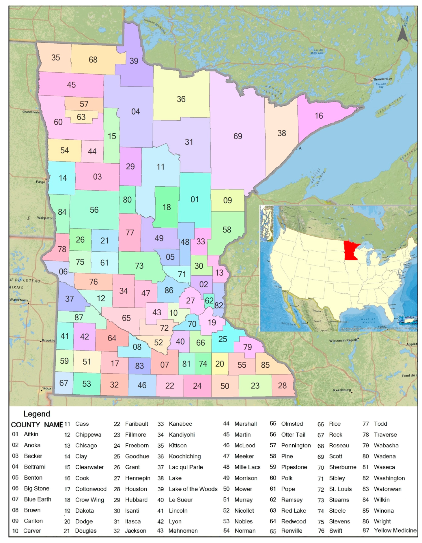
Figure 1. Map of counties in the state of Minnesota.
Remotesensing 12 03955 g001
Figure 2. Framework of multidimensional ecosystem services assessment.
Remotesensing 12 03955 g002
Figure 3. Flowchart of image processing.
Remotesensing 12 03955 g003
Figure 4. Distribution and change of multidimensional assessment results.
Remotesensing 12 03955 g004
Figure 5. Changes in P-score, Q-score, and D-score.
Remotesensing 12 03955 g005
Figure 6. Multidimensional assessment geospatial results.
Remotesensing 12 03955 g006
Figure 7. Spatial distribution of P-score (total output of food provisioning ecosystem services).
Remotesensing 12 03955 g007
Figure 8. Spatial distribution of Q-score (efficiency of food provisioning ecosystem services).
Remotesensing 12 03955 g008
Figure 9. Spatial distribution of D-score (trend of food provisioning ecosystem services).
Remotesensing 12 03955 g009
Table 1. Multidimensional assessment spaces and their properties.
SpacePQDPropertiesDescription
I+++The total output, efficiency, and trend index are above average.Progression
II++The total output and efficiency are above average, but the trend index is below average.Degradation
III++Although the efficiency is below average, it has been raised. The above-average output depends on the larger ecosystem area.Progression
IV+The efficiency is below average and it has degraded. The above-average output depends on ecosystem scales.Degradation
V++The output is below average, indicating that the ecosystem scale should be expanded.Progression
VI+Both the output and the trend index are below average, but it has high efficiency.Degradation
VII+The output and efficiency are below average, but it has an above-average trend index.Progression
VIIIAll three indices are below average. It has a lower output and efficiency. Simultaneously and unfortunately, it has degraded.Degradation
Table 2. Formulas of assessment indices.
IndexFormulationIntroduction
P P i j = P i j P j ¯ σ P j P i j is P-score of county i in the year j, P i j is the crop production of county i in the year j,   P j ¯ is the average crop production of the state in year j, σ P j is the crop production standard variance of all counties in year j.
Q Q i j = Q i j Q j ¯ σ Q j Q i j is the Q-score of ecosystem service efficiency of county i in the year j, Q i j is the yield of county i in the year j, Q j ¯ is the average crop yield of the state in year j,   σ Q j   is the yield standard variance of all counties in year j.
D D i j = D i j D j ¯ σ D j
D i j = Q i j Q i ( j 1 )
D i j is the D-score of the county i in the year j, D j ¯ is the annual efficiency change in county i in year j, is the average of annual efficiency change in the entire state in year j, σ D j is the annual efficiency change standard variance of all counties in year j.
Table 3. Critical p and critical z values with different confidence levels.
Z Score (Standard Deviation)p Value (Probability)Confidence Level
z < −1.65 or z > +1.65p < 0.190%
z < −1.95 or z > +1.95p < 0.0595%
z < −2.58 or z > +2.58p < 0.0199%
Table 4. Agricultural districts in Minnesota.
Agricultural DistrictCounties
CentralScott, Wadena, Sherburne, Morrison, Renville, Todd, Meeker, McLeod, Wright, Benton, Sibley, Carver, Stearns, Kandiyohi
East CentralAitkin, Hennepin, Ramsey, Crow Wing, Carlton, Washington, Pine, Isanti, Anoka, Mille Lacs, Chisago, Kanabec
North CentralKoochiching, Cass, Lake of the Woods, Hubbard, Itasca, Beltrami
NortheastCook, Lake, St. Louis
NorthwestBecker, Clay, Marshall, Red Lake, Norman, Roseau, Mahnomen, Polk, Pennington, Kittson, Clearwater
South CentralFaribault, Martin, Rice, Blue Earth, Waseca, Watonwan, Brown, Le Sueur, Freeborn, Nicollet, Steele
SoutheastDodge, Winona, Mower, Wabasha, Goodhue, Houston, Dakota, Fillmore, Olmsted
SouthwestCottonwood, Redwood, Murray, Rock, Lyon, Jackson, Nobles, Lincoln, Pipestone
West CentralWilkin, Traverse, Yellow Medicine, Grant, Chippewa, Swift, Otter Tail, Stevens, Lac qui Parle, Big Stone, Douglas, Pope
Table 5. Principal component loads.
VariablesPrincipal Component
Z 1 Z 2 Z 3
PDI0.56440.1860−0.0430
NDVI0.18700.53650.7947
RF0.5970−0.0340−0.2448
DT0.5375−0.38960.0750
DIF0.03370.7243−0.5487
Table 6. F-test results.
Objects α F ScoreCritical ValueResults
P0.00523.463.76credible
Q0.00514.193.76credible
D + 0.12.911.92credible
D 0.13.251.92credible
Publisher’s Note: MDPI stays neutral with regard to jurisdictional claims in published maps and institutional affiliations.