Article

RGB Image Prioritization Using Convolutional Neural Network on a Microprocessor for Nanosatellites

1
Institute for Space-Earth Environmental Research, Nagoya University, Nagoya 464-8601, Japan
2
Department of Aerospace Engineering, Nagoya University, Nagoya 464-8601, Japan
3
PASCO CORPORATION, Tokyo 153-0043, Japan
4
NTT DATA Mathematical Systems Inc., Tokyo 160-0016, Japan
5
NAVER LABS Corporation, Seongnam 13638, Korea
*
Author to whom correspondence should be addressed.
Remote Sens. 2020, 12(23), 3941; https://doi.org/10.3390/rs12233941
Submission received: 5 November 2020 / Accepted: 26 November 2020 / Published: 3 December 2020

Abstract

:
Nanosatellites are being widely used in various missions, including remote sensing applications. However, the difficulty lies in mission operation due to downlink speed limitation in nanosatellites. Considering the global cloud fraction of 67%, retrieving clear images through the limited downlink capacity becomes a larger issue. In order to solve this problem, we propose an image prioritization method based on cloud coverage using CNN. The CNN is designed to be lightweight and to be able to prioritize RGB images for nanosatellite application. As previous CNNs are too heavy for onboard processing, new strategies are introduced to lighten the network. The input size is reduced, and patch decomposition is implemented for reduced memory usage. Replication padding is applied on the first block to suppress border ambiguity in the patches. The depth of the network is reduced for small input size adaptation, and the number of kernels is reduced to decrease the total number of parameters. Lastly, a multi-stream architecture is implemented to suppress the network from optimizing on color features. As a result, the number of parameters was reduced down to 0.4%, and the inference time was reduced down to 4.3% of the original network while maintaining approximately 70% precision. We expect that the proposed method will enhance the downlink capability of clear images in nanosatellites by 112%.

Graphical Abstract

1. Introduction

Nanosatellite is a classification of small satellites ranging from 1–10 kg. Multiple nanosatellites can be operated as a constellation due to its low cost, allowing missions to achieve high spatial resolution by multipoint observation and high temporal resolution by short revisit time. Due to these reasons, nanosatellites have been used in various missions [1] such as atmosphere exploration [2] or remote sensing applications [3,4]. Especially in remote sensing, recent nanosatellites have been delivering 3.7 m resolution images [5]. Combining such imaging performance with the advantages of nanosatellites opens a new space era allowing near-real time global coverage Earth observation capabilities. However, nanosatellites have limited resource (i.e., electrical power or payload mass/volume) due to its size compared to conventional satellites, restricting nanosatellite operations related to electrical power or data downlink capability. According to Figure 1, although many commercial application nanosatellites have achieved high data rates, yet many of the academic nanosatellites do not have access to the high-end transmitter or ground station facilities, which limit typical nanosatellite systems in downlinking only a few images daily.
In the case of remote sensing applications over regions with high cloud fraction, the downlink limitation of nanosatellites becomes a larger problem when it comes to retrieving clear images if only a few images can be downloaded. According to a previous study [23], approximately 67% of the land is covered with clouds, and local regions with high cloud fraction exceeding 80% exist. This implies that depending on the region, there is a high possibility that downlinked images will contain cloudy scenes, reducing the effective downlink of nanosatellites.
In order to solve this problem, we aim to accomplish cloudy image rejection by implementing clear image prioritization and discarding lower priority images based on cloud coverage. Cloud coverage estimation in remote sensing has been an active research area, however many research uses additional bands [24,25,26], or the methods are computationally too heavy for onboard processing [27,28,29,30]. As previously introduced, nanosatellites are miniaturized platforms; therefore it is difficult to board additional payload. Thus an optimal nanosatellite system would be a system capable of estimating cloud coverage using what is onboard, which is typically an imager with RGB channels. Furthermore, to prioritize the images, all images should be processed onboard, which requires the cloud coverage estimator to run in nanosatellites.
Considering a nanosatellite with an onboard imager with a FOV (Field of View) of 50 km and further assuming that the images are captured every 50 km during daylight, approximately 6400 images would be generated daily. Such operation requires each image to be processed within 13.5 s using the embedded computer onboard the nanosatellite. Therefore in this study, our requirements are specified to use only RGB images and to be able to run in microcontrollers. Accordingly, the main contribution of the paper is the development of lightweight CNN for onboard image prioritization only using RGB images. We propose a novel method with multiple strategies to meet the requirements: (1) Using thumbnail input images, (2) using patch decomposition, and (3) miniaturizing the CNN (Convolutional Neural Network) architecture. A multi-stream CNN is developed to suppress overfitting of the model to color features, with reflection padding implemented on the first block of the convolutional layers to minimize noise from the border of the images. In Section 2, related work is introduced, and the problems in applying conventional methods are identified. The methods used in the study is introduced in Section 3. The formulation of the proposed method, image evaluation and accuracy metric, and dataset generation method are described in detail. Sensitivity analysis of the proposed strategies, and the computational cost are analyzed in Section 4. Examples of image prioritization results are also presented in the section. The limitations of the proposed method and potential future work are described in Section 5. Lastly, the proposed study is summarized in Section 6.

2. Related Work

Cloud coverage estimations have been among many tasks within post processing in the remote sensing community for automated data analysis. Automated data analysis required masking techniques, in which conventional cloud coverage estimation methods used algorithms involving multiple spectral band inputs.
As part of the LDCM (Landsat Data Continuity Mission) CCA (Cloud-Cover Assessment), ACCA (Automated Cloud-Cover Assessment) was developed [31,32] to build Landsat archive for data management. ACCA incorporates two steps in pixel-wise cloud assessment. The first step consists of a decision tree using five bands and the second step consists of refinement using thermal analysis. However, weakness over cloud shadow, reflectance, or temperature inversion were found in the ACCA algorithm. LDCM (Landsat Data Continuity Mission) followed the LTAP, and new algorithms including Expanded AT-ACCA (Artificial Thermal Automated Cloud-Cover Assessment) and C5 CCA were developed to overcome the disadvantages of the ACCA algorithm. The Expanded AT-ACCA algorithm was developed to evaluate the CCA without the thermal band by modeling the AT (Artificial Thermal) band using the reflective bands [33]. The use of AT removed the dependency of the thermal band from ACCA, allowing CCA even when TIRS (Thermal Infrared Sensors) data were unavailable. However, due to a large number of pixel ambiguity, an additional routine of a simple McCulloch-Pitts neural network was involved to classify the ambiguous pixels in AT-ACCA. Whereas the Expanded AT-ACCA is based on ACCA involving multiple passes for CCA, C5 CCA was developed using a statistical classifier C5.0 to create a stand-alone decision tree [33]. Despite the limited training data size due to memory errors, C5 CCA outperformed ACCA even without the thermal band present. However, the high sensitivity depending on differences in the spectral bandwidth, and maintenance problem due to the algorithm’s complexity remained as potential problems for C5 CCA.
Fmask (Function of mask) [24,25] was introduced to improve the performance of cirrus and cloud shadow detection over conventional methods used on Landsat images. Fmask uses six TOA (Top of Atmosphere) reflectance bands (Bands 1, 2, 3, 4, 5, 7) and a BT (Brightness Temperature) band (Band 6) as the input from the Landsat images. The potential cloud/shadow/snow layers are first identified using a combination of spectral tests, and geometric information is used for matching the overlap of potential cloud/shadow layers with cloud shadow objects to generate the final cloud/shadow masks. The additional matching algorithm by augmenting geometric information showed significant improvement in cloud mask accuracy. However, Fmask showed limitations in very bright or very cold land features due to the high sensitivity of the algorithm on the BT.
A time-series method was introduced to improve the cloud and cloud shadow screening in Landsat images by further using temporal information in addition to spectral and contextual information [34]. The method incorporates four passes: the first and second passes detect cloud affected pixels using minimal and median difference in band 1 over the temporal data, third pass detects shadow affected pixels using the median difference in bands 4 and 5, and the fourth pass classifies the shadow affected pixels by examining shadow objects. Although the time series method shows better cloud and cloud shadow screening accuracy over Fmask, the method was not evaluated under the same scene optimization between the time series method and the Fmask. A clear limitation of the time series method remains due to temporal data requirement, which is typically unavailable on online cloud and cloud shadow screening applications.
More recent methods introduced extensive use of machine learning to achieve a more efficient and reliable cloud and cloud shadow masking. SPARCS (Spatial Procedures for the Automated Removal of Clouds and Shadows) used a neural network with Landsat ETM+ bands 1 through 7 [35] as the input. Further spatial post-processing on the network output with a set of rules on ambiguous pixels was performed to reduce classification error. SPARCS outperformed Fmask on classifying cloud shadow, snow/ice, and clear pixels, showing the potential of machine learning techniques. Wei [36] developed a two-stage method named RFmask, which uses RFC (Random Forest Classification) and SEEDS (Super-pixels Extracted via Energy-Driven Sampling). RFmask uses RFC first to perform pixel level classification, and then the SEEDS to perform spatial analysis. The RFC used multispectral band data from Landsat 7 and Landsat 8 as basic input features, and spectral indices and brightness index were additionally derived from the basic input features. RGB image combined using the red, green, and blue channel of Landsat image is input to SEEDS for spatial segmentation of potential objects. Then RFC and SEEDS results are laid together, generating the final cloud mask. RFmask outperformed conventional methods and also showed comparable results with deep learning methods. However, RFmask omitted small cloud with less pixels due to SEEDS, and the accuracy of snow/ice was low.
Deep learning methods were introduced as the computational power increased over time. Most of the teams used CNN [37] to learn the spatial characteristics, as the convolution layers in CNN are best suited in extracting spatial features. The spatial features allow the CNN to distinguish deeper features such as shape or texture, which grant CNN the outstanding ability in performance over conventional methods based on pixel-wise classification. Shi and Liu [38,39] used CNN as a classifier on superpixels. The superpixels help reduce computation time and noise by taking advantage of group-level statistics. Both Shi and Liu used SLIC (simple linear iterative clustering) [40] for clustering the superpixels and further implemented refinement techniques to solve ambiguous superpixel problems. Shi [38] implemented a gradient method for the superpixels on the classification results to improve the accuracy near the cloud boundaries. The gradient method compares the cloud probability of a superpixel to neighboring superpixels, and the superpixel is refined for large gradient values. Liu [39] combined HFCNN (Hierarchical Fusion CNN) and deep forest to classify superpixels, and further implemented ambiguous superpixel refinement by introducing a distance matrix. The distance matrix calculates the distance metric of cirrus against cloud and other classes, which then the cirrus is refined as cloud depending on the relative distance against neighboring superpixels. Although both methods showed high accuracy above 0.9, using superpixels has large error resolution at superpixel levels, which show high sensitivity for large superpixels.
On the other hand, pixel-wise image segmentation methods using CNN were also investigated [26,29,41]. The U-Net architecture [42] or its variants were used as the baseline CNN model. Drönner [26] developed a CS-CNN (Cloud Segmentation CNN), varying U-Net by reducing the number of kernels, implementing pooling layers using convolution layers with strides, and adding dropout layers. The variations were made to reduce computational time, learn layer-specific downsampling operations, and prevent overfitting respectively. The CS-CNN was evaluated against various input bands of SEVIRI, which showed that IR channels were sufficient in generating robust cloud masks with accuracies as high as 0.948. The addition of VNIR channels showed significant improvement only in snow/ice masks. Jeppesen [29] developed RS-Net, a variant of U-Net, with batch normalization after each convolutional layer in the encoder and cropping layer after the final layer. Batch normalization was added to speed up the training of the CNN and the cropping layer was added to discard the borders where spatial information is lacking during the convolutional layers. Jeppesen also evaluated various combinations of Landsat 8 bands, including combinations consisting only of visual bands (RGB). The results showed that RS-Net outperformed Fmask, and furthermore, RGB band classification showed promising results. Zhang [41] developed a lightweight CNN named L-Unet based on U-Net. Four bands from Landsat 8 including three visual bands and an additional infrared band (bands 2, 3, 4, 5) were used. Zhang implemented LeGall-5/3 wavelet transform for input image compression in order to reduce the computational cost. L-Unet was tested on Raspberry Pi, showing the feasibility of lightweight CNN on systems with low computational power.
Although there was much progress in cloud coverage estimation methods, previous methods use multiple bands, and the methods are too heavy to be implemented onboard a nanosatellite. Therefore, a new method for extremely low computational power and limited band must be developed to achieve onboard cloud coverage estimation on a nanosatellite. Accordingly, we develop a lightweight CNN-based cloud coverage ranking method using only RGB bands as the input.

3. Methods

In this section, we introduce the methods used throughout the study. The overview of the flowchart of the proposed method is shown in Figure 2. Preprocessing is performed to reduce the computational cost and resource requirement of the CNN. A lightweight CNN is then used to predict the cloud coverage of each patch. Lastly, the input image is prioritized based on cloud coverage fraction evaluation of all the patches. The following subsections introduce the formulation of the proposed method, image evaluation method, accuracy metric, and dataset generation method in detail.

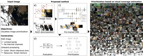
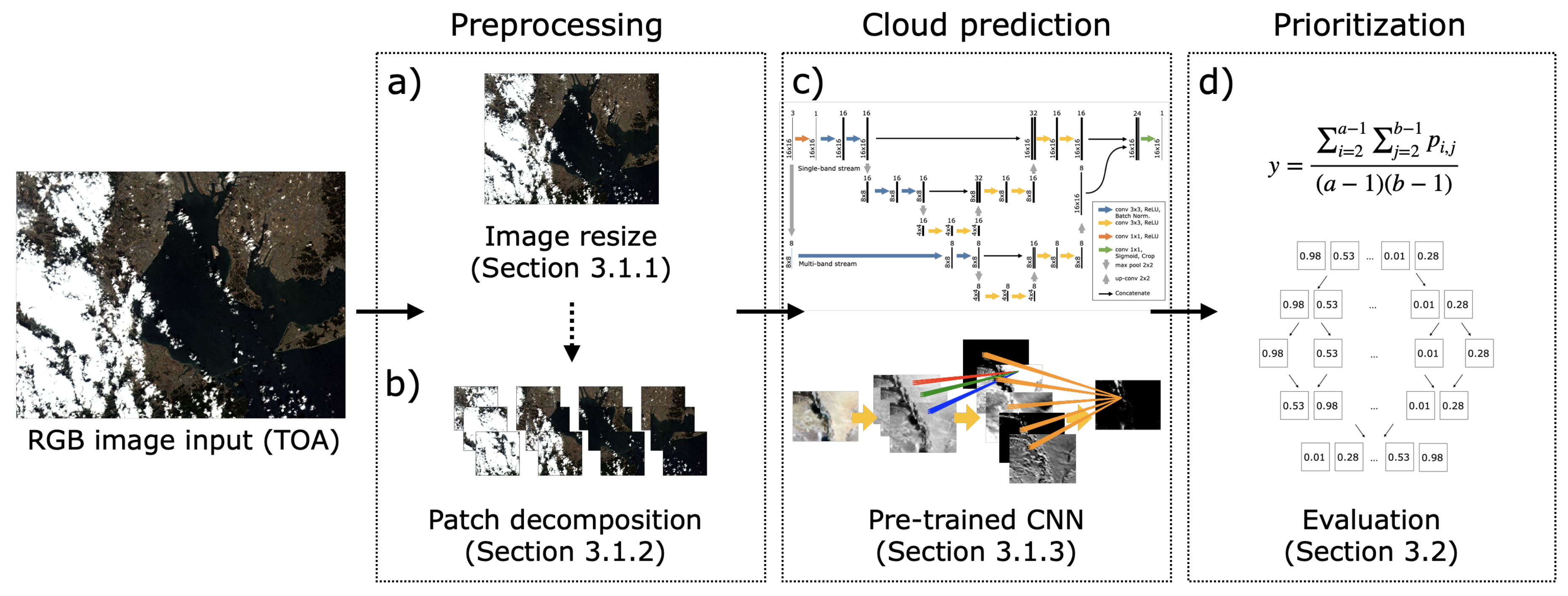
3.1. Proposed Method

As previously introduced, the proposed work focuses on image prioritization onboard a nanosatellite, therefore processing speed and accuracy are both important criteria. In our method, three strategies are adopted to meet the criteria: (1) Reduction of input size, (2) Input decomposition into patches, and (3) miniaturization of the CNN architecture. This section describes each of the strategies in detail.

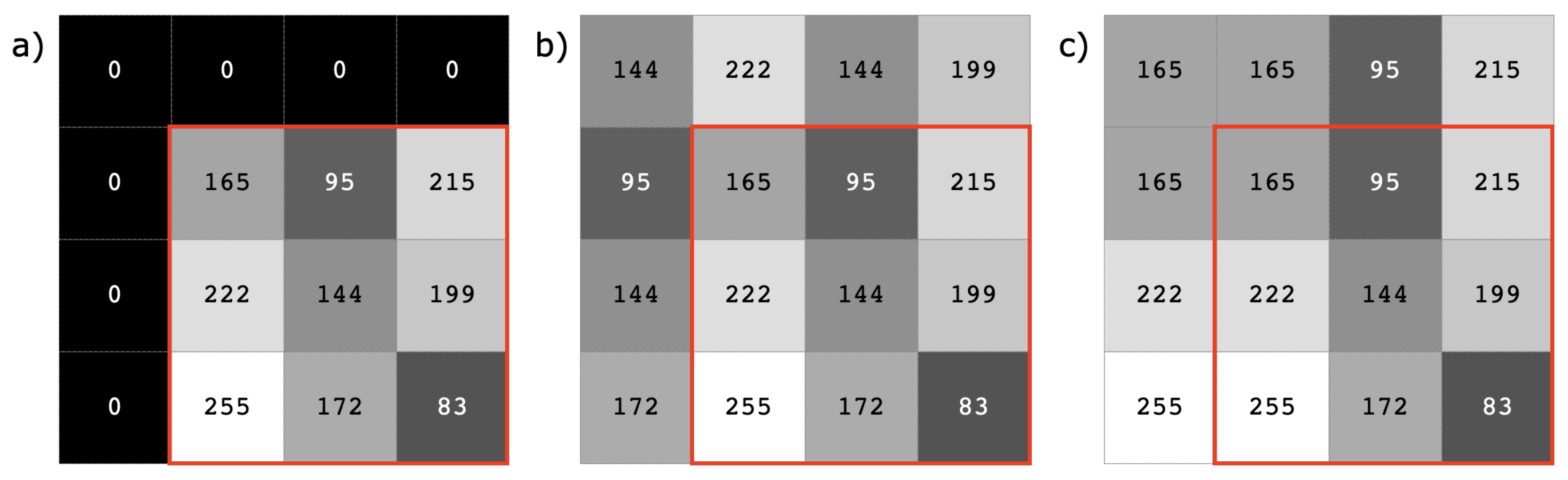
3.1.1. Input Size Reduction

One of the most direct methods of reducing computational cost is to reduce the size of the input. Considering a single simple convolution layer, the number of operations required is proportional to the input size. As the same applies to consecutive layers, the overall operation is approximately proportional to the size of the input. Comparing a 5 MP image (2592 × 1944) and a VGA image (640 × 480), the 5 MP image would require approximately 16 times longer computational time. In this study, VGA images are resized to 64 × 48 images, which reduces the base computational cost down to a hundredth. An additional aspect is that, along with computational advantages, reduced input size allows the network to train on small images. Such a feature makes the fine tuning process after the nanosatellite is placed into orbit easier, as more thumbnail images can be downloaded for training compared to original images. Despite the computational and training advantages, it should be noted that input reduction degrades the image resolution, resulting in cloud coverage estimation accuracy of CNN to decrease as the CNN will not be able to learn from small features.

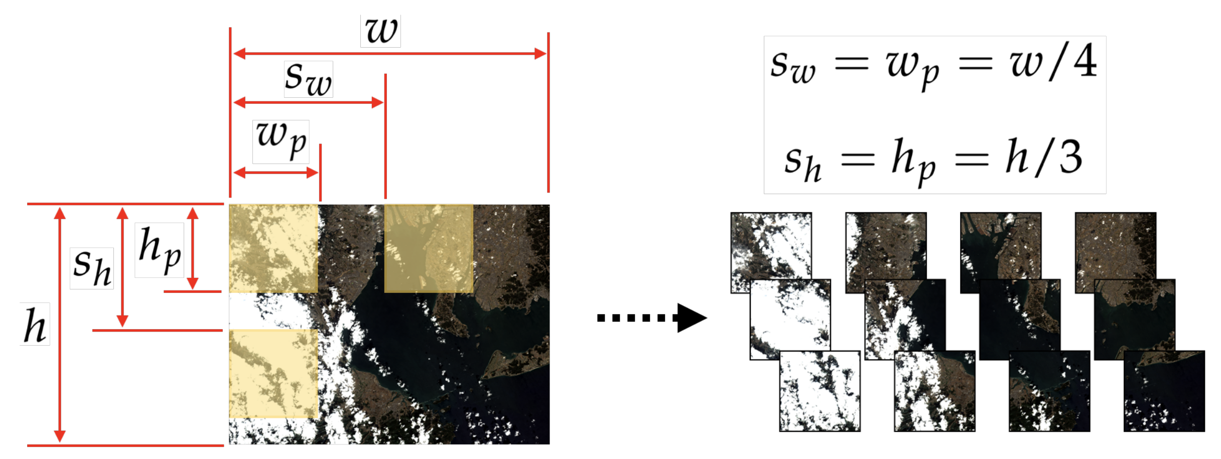
3.1.2. Patch Decomposition

In this study, patch decomposition is implemented for further slicing the input into smaller size patches. Calling small patches at a time requires less memory and reduces the runtime of each task onboard. Such characteristics have advantages in space environment, as memory is subject to possible bit flips due to single events, and tasks with short runtime increase the flexibility in task scheduling in embedded systems. Furthermore, by using patch decomposition, a single image can be handled in parallel by multicore microprocessors.
x ( m ) = w w p s w + 1 × h h p s h + 1
The number of patches of an image with a size of w×h×c is shown in Equation (1) for patch size of w p × h p ×c with width-wise stride s w and height-wise stride s h , where x ( m ) is the number of patches. Note that the division in Equation (1) is an integer division. As an example, a 640 × 480 × 3 image with 32 × 32 × 3 patch and a 32 × 32 stride would extract 300 patches, whereas the target input and patch size of this study are a 64 × 48 × 3 image with 16 × 16 × 3 patch and a 16 × 16 stride, which extract 12 patches as shown in Figure 3.
However, as discussed by Jeppesen [29], loss in the outermost boundary of the input due to lack of information outside of the boundary becomes a larger problem when using patch decomposition. Jeppesen proposes cropping out the boundaries where the most uncertainty lies. Considering the cropped pixels against the total pixels of the image with a size of a × b , the ratio η is given as Equation (2).
η = 2 ( a + b 2 ) a b
For a fixed pixel size patch, the border ratio is the smallest when a and b are equal, i.e., a perfect square. Therefore in this study, we choose patch candidates with perfect squares. In the case of a patch input with a size of 16 × 16 , the uncertainty due to the cropped boundary is approximately 23.5%. Thus, the tradeoff between computational cost and accuracy must be considered carefully when using patch decomposition.

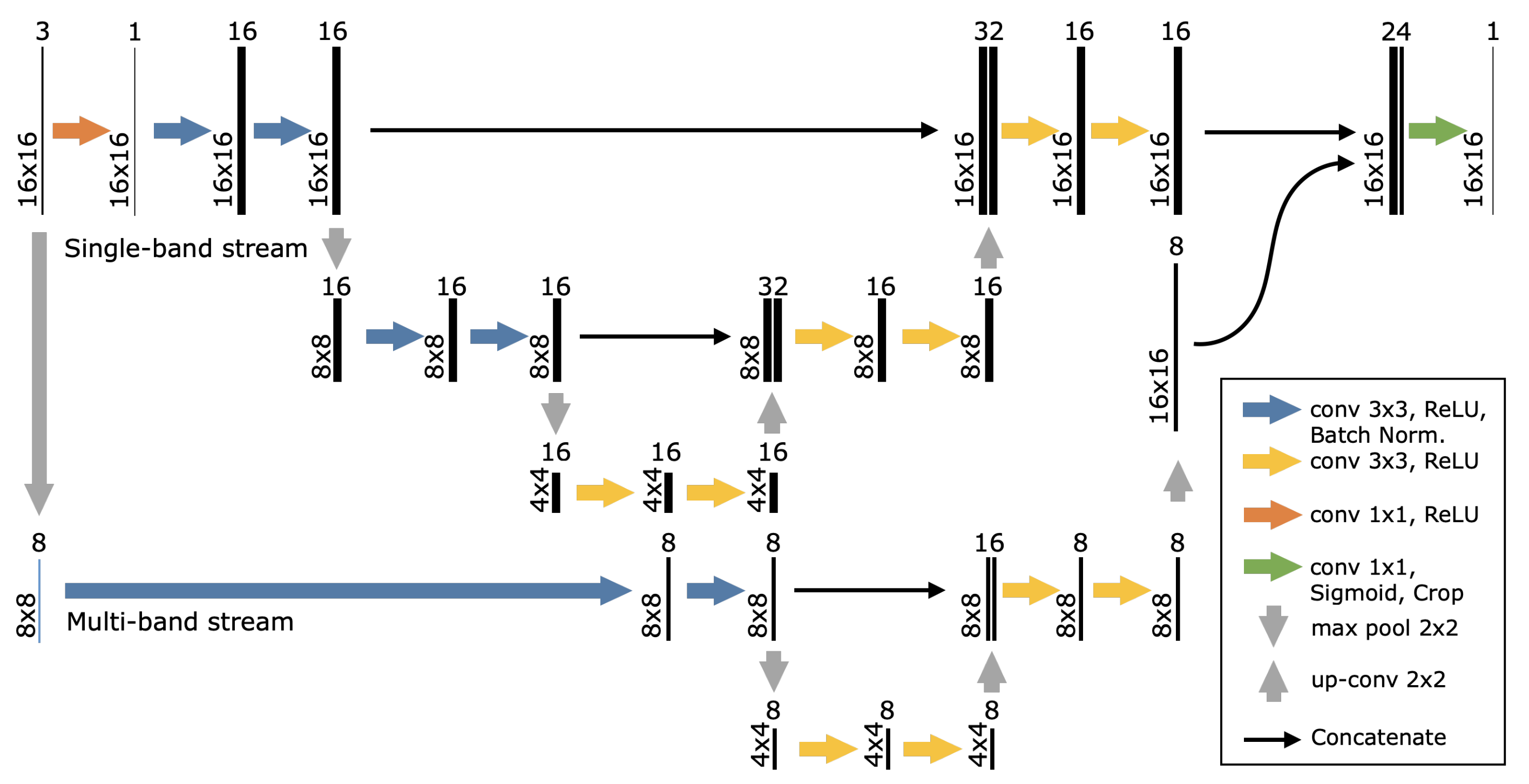
3.1.3. CNN Architecture Miniaturization

In this study, CNN (Convolution Neural Network) [37] is used for cloud coverage estimation. Jeppesen [29] showed that RS-Net works well with remote sensing images, as introduced in Section 2. However, the strategies used in this study involves input size reduction and further decomposing the resized input into smaller patches. Due to the reduced input size, the maximum possible number of pooling operations is limited to twice. Furthermore, the number of kernels in each convolution layer in RS-Net makes the network heavy for microcontrollers. Therefore the number of Kernels in each of the convolutional layers are reduced.
As a result of modifying the base structure of CNN matching the input, the CNN also becomes shallower, and the decreased number of kernels limits the number of features in the hidden layers. In the proposed method, we develop a multi-stream architecture to assure the network to learn spatial features and suppress the network from optimizing against color features. The multi-stream forwards the input to a single-band stream and a multi-band stream. A deeper and larger network is constructed for the single-band stream to mimic panchromatic images and extract spatial features. The single-band stream consists of a (1 × 1) convolutional layer to transform the input into a single-band image. A custom kernel constraint is defined, such that the sum of the weights does not exceed a unit value with bias set to zero. The multi-band stream feeds the input directly into a pooling layer to match the output size of the single-band stream. The single-band and multi-band stream outputs are concatenated at the end of the CNN.
The padding for the first block in each of the streams is further modified to improve the performance near the border of the input patches. The proposed method is subject to errors at the borders of the patches, as described in Section 3.1.2. The typical zero-padding in the convolutional layer would underestimate the cloud coverage, as zeros are interpreted as non-cloudy features in the convolutional layers. Underestimation in cloud rejection applications is unwanted, as it will degrade the precision of the network. As a solution, the zero-padding in the convolutional layers are replaced by replication padding, with an assumption that natural clouds are spatially continuous. Replication padding is only applied in the first convolutional blocks of each of the streams, as deeper layers have higher-order derivation error due to propagation. The different types of paddings are depicted in Figure 4.
The rest of the CNN architecture resembles RS-Net, except for the aforementioned modifications. Batch normalization is applied after each activation in the downsampling convolutions, and sigmoid with zero bias is used as the activation function of the last convolutional layer. The proposed network is called NU-Net (Nano U-Net). The architecture of NU-Net is shown in Figure 5. NU-Net shrinks RS-Net from 7,854,592 parameters down to 29,907 parameters, reducing the number of parameters down to merely 0.4% of the original network.

3.2. Image Evaluation

The segmentation result of NU-Net is converted to cloud coverage by evaluating the confidence value of each pixel. The cloud coverage of a single patch is given in Equation (3), where y, a, b, p represents the cloud coverage of a single patch, width of the patch, height of the patch, and the pixel value.
y = Σ i = 2 a 1 Σ j = 2 b 1 p i , j ( a 1 ) ( b 1 )
The image cloud coverage is evaluated by taking the average of all the subset patches of the image as given Equation (4), where Y, m, y represents the cloud coverage of an image, number of patches in an image, and the cloud coverage of a single patch respectively. The images are finally prioritized based on the cloud coverage of each image. Merge sort algorithm is used in this study for the ranking of the images for prioritization.
Y = 1 m Σ i = 0 m y i

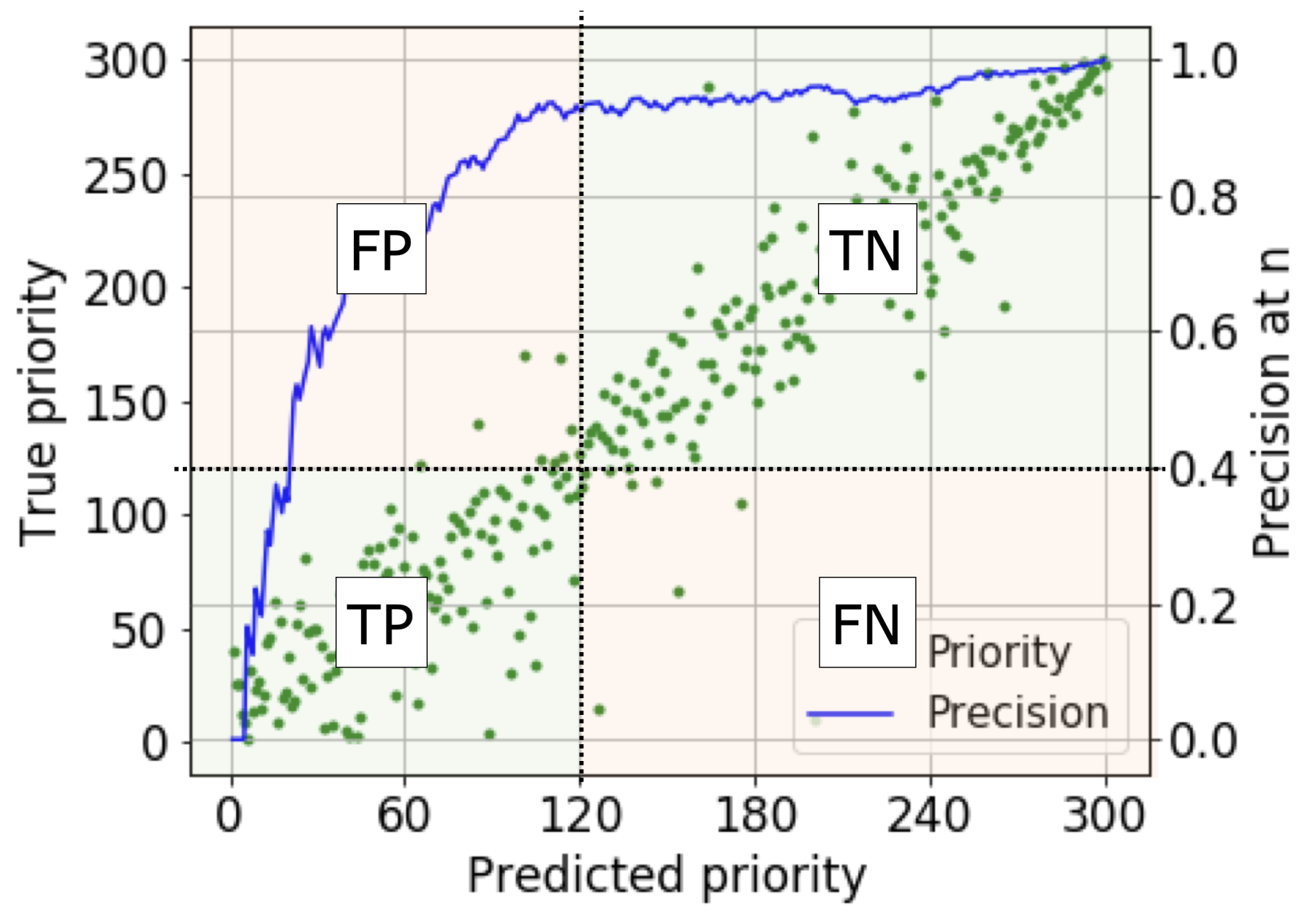
3.3. Accuracy Metric

Prior to presenting the results, as it is difficult to quantify and assess the performance over prioritization, the accuracy metric must be defined. The precision at n [43] for both cloud coverage and priority is evaluated to quantify the results. The precision at n of cloud coverage shows the network characteristics against the cloud coverage spectrum, and the precision at n of priority shows the prioritization performance of the test dataset when n images are downlinked.
Figure 6 shows an example of precision at 0.4 for cloud coverage. The first quadrant is defined as true negative (TP), as the true cloud coverage of the images is higher than 0.4. The second quadrant is defined as false positive (FP), as these images were predicted to have cloud coverage lower than 0.4, whereas the true cloud coverage is higher than 0.4. The third quadrant is defined as true positive (TP) as the true cloud coverage is less than 0.4. Lastly, the fourth quadrant is defined as false negative (FN), as the images were predicted to have cloud coverage higher than 0.4, whereas the true cloud coverage is less than 0.4. The top accuracies are evaluated at small steps to cover the whole spectrum, which finally gives the precision at n curve. In this study, the accuracy is measured against precision, as it is more important not to download any cloudy images rather than missing clear images. In the case of a one-to-one correspondence ranking problem, precision and recall are the same as the number of false negative and false positive cases is the same.
Besides the accuracy metric, the Spearman’s rank correlation coefficient is calculated for evaluating the predicted priority rank against the true priority rank. The Spearman’s rank correlation coefficient quantifies the correlation between the two ranks. The equation for the Spearman’s rank correlation coefficient is given in Equation (5), where ρ , d i , n represents the spearman’s rank correlation coefficient, the difference in paired ranks, and the number of paired ranks, respectively.
ρ = 1 6 Σ d i 2 n ( n 2 1 )
As precision at n is affected by the distribution of the testing dataset, the proposed method is evaluated against testing dataset generated by images with various cloud coverage distributions.

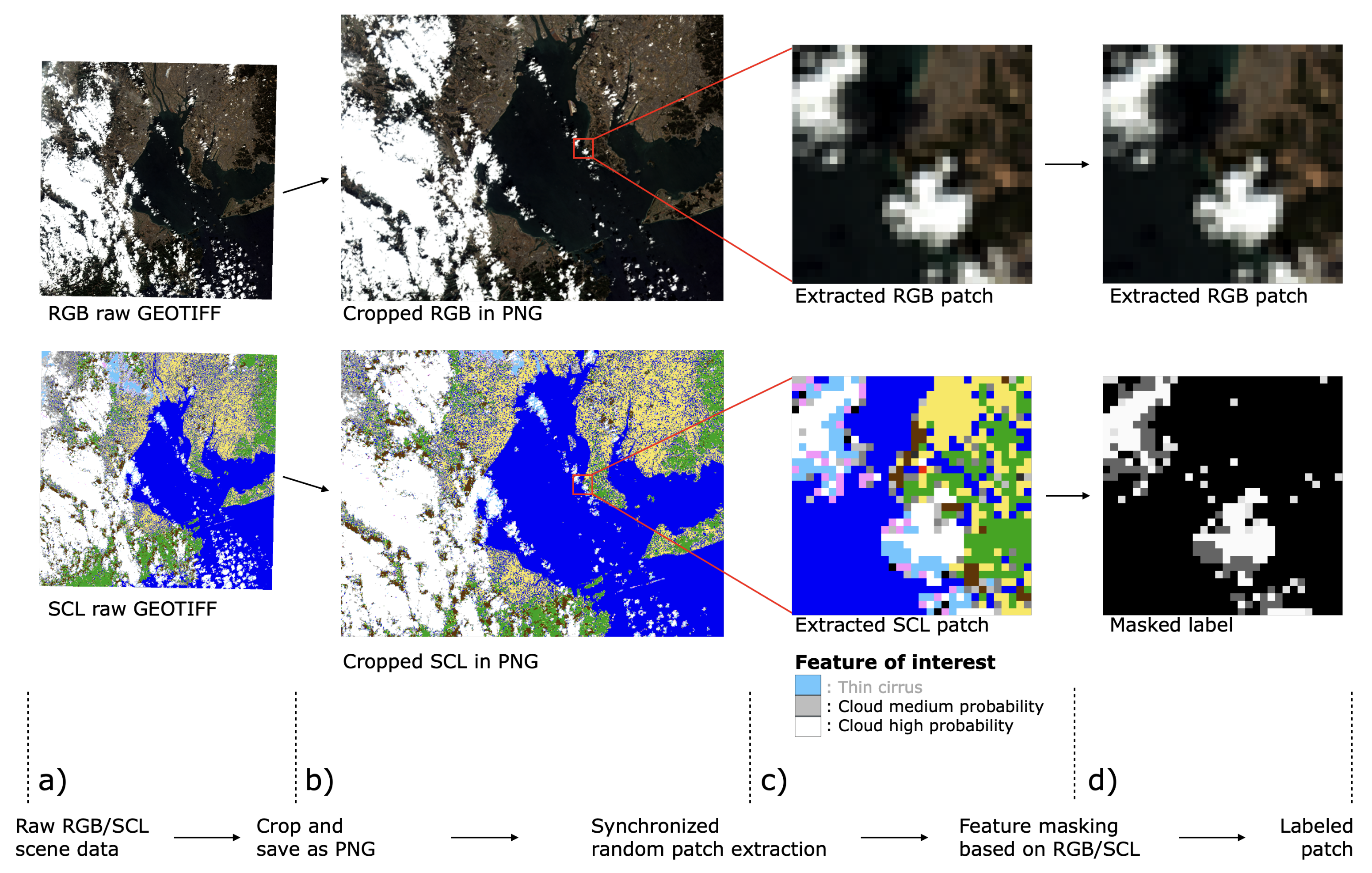
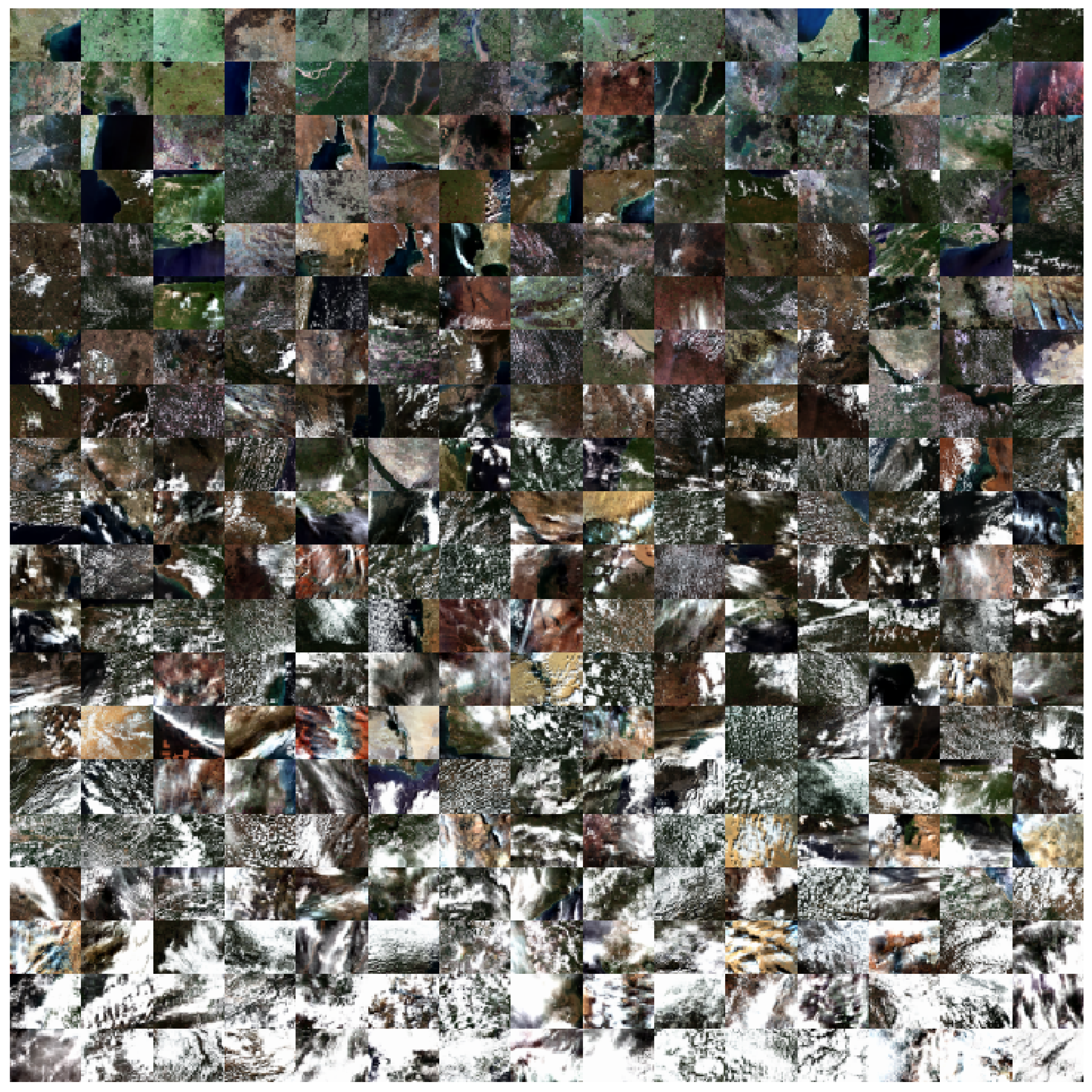
3.4. Dataset Generation

3.4.1. Automatic Dataset Generation
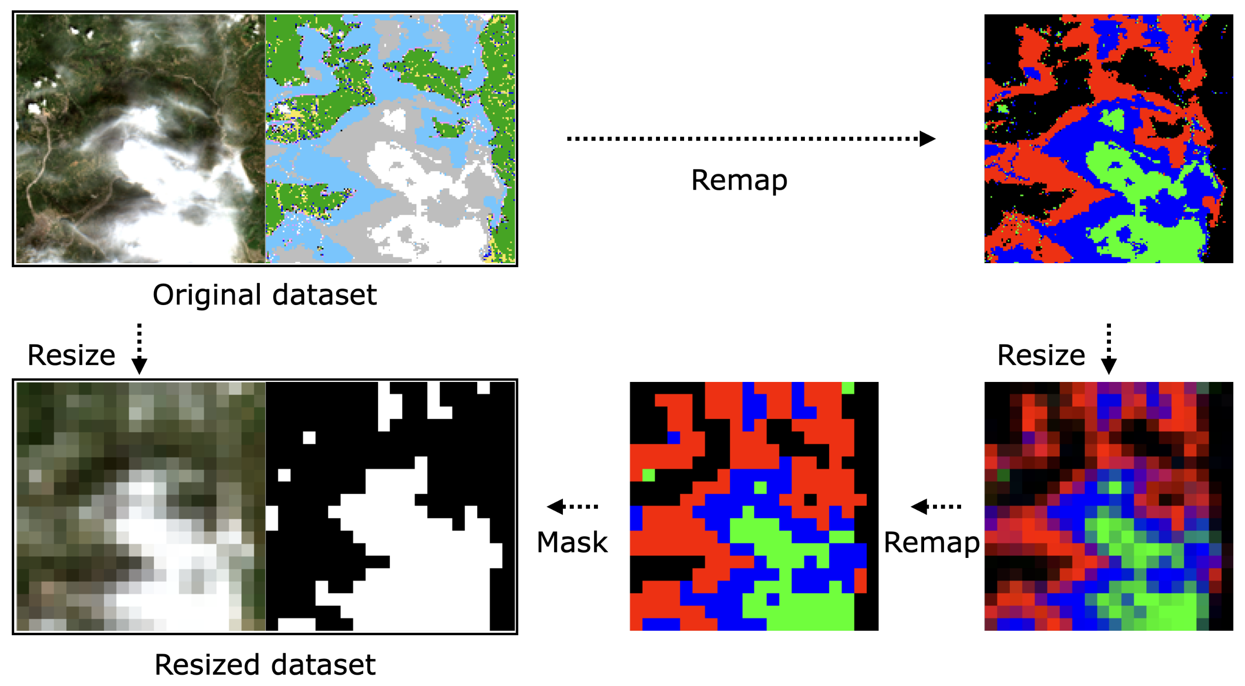
Manual labeling increases the overall cost during training, validation, and testing of a neural network, and the cost increases when the application becomes related to semantic segmentation. In this study, an automatic data labeling method is developed using scene classification satellite products from Sentinel-2 [44] to reduce the cost. TCI (True Color Image) and SCL (Scene Classification map) products are used as a set [45] for automatic dataset generation. Sentinel-2 TCI provides the RGB data, which resembles RGB images acquired by nanosatellite imagers. In this study, low resolution images corresponding 60 m resolution images were used to mimic the performance of nanosatellite imagers. Sentinel-2 SCL provides the ground truth for the corresponding TCI with information on scene features, including cloud.
The input raw images, consisting of a set of TCI and SCL products from Sentinel-2, are converted and cropped to generate a baseline image set, as shown in Figure 7a,b. Once the baseline image sets are generated, patches are extracted depending on the patch decomposition parameters described in Section 3.1.2. During the extraction of patches, the same sector is extracted from the baseline image set, as shown in Figure 7c. Finally, a grayscale mask is generated based on features of interest, and the final cloud mask is generated as shown in Figure 7d.
In this study, 600 images were used with 300 images allocated for the training dataset and 300 images allocated for the test dataset. Within the training dataset, 70% were allocated for training, and 30% were allocated for validation. The training and test dataset are provided as supplementary material Data D1.

3.4.2. Label Resize

In the proposed method, the input images are resized to reduce the total arithmetic operations. However, a problem with the input size reduction is the dataset preparation for the CNN. When using the dataset generation method introduced in Section 3.4, resizing the SCL will mix the features nearby each other, resulting in inaccurate feature mapping during the masking process in Figure 7d.
To overcome the resize problem, the SCL patch is reconfigured such that features of interest are distributed to each of the channels of the image. If multiple features share a channel, it would be difficult to decompose the features after the resize. In this study, as we are only interested in thin cirrus, high probability cloud, and medium probability cloud, the three labels are remapped to the red, green, and blue channels. The resize process is shown in Figure 8.

4. Results and Discussion

Unless mentioned separately, this section presents results from NU-Net with an input image size of 64 × 48 × 3 with patch size of 16 × 16 × 3. The network was trained with a learning rate of 1 × 10 4 , L2 regularization of 1 × 10 3 , and without any dropout.

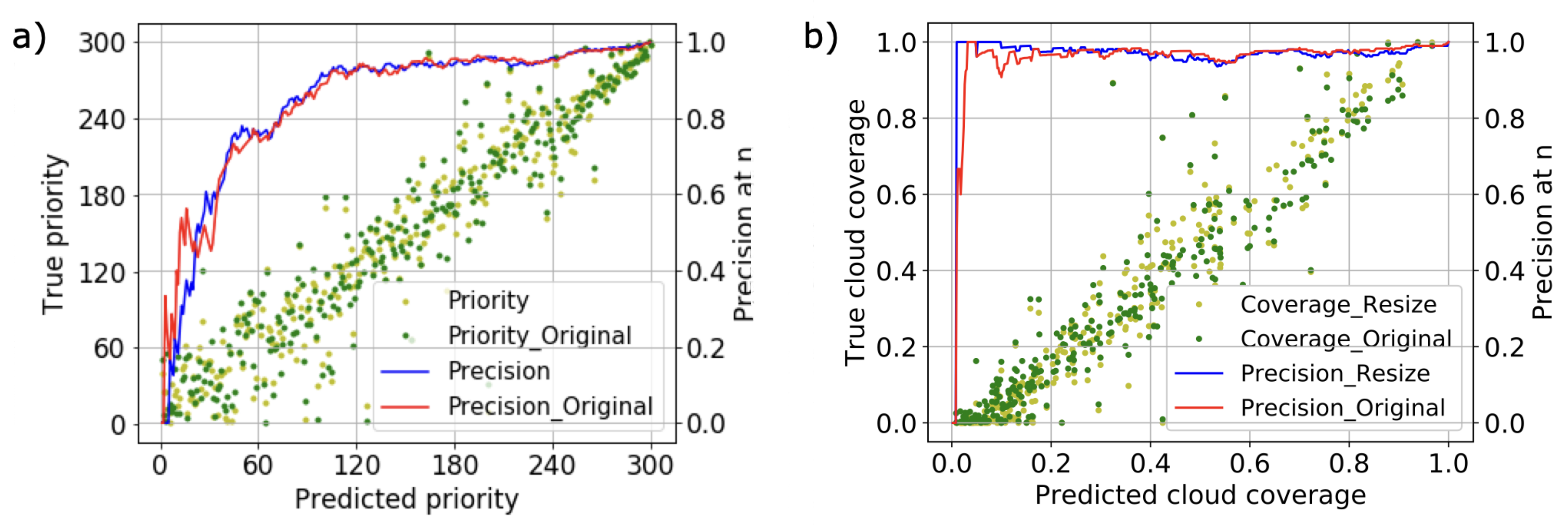
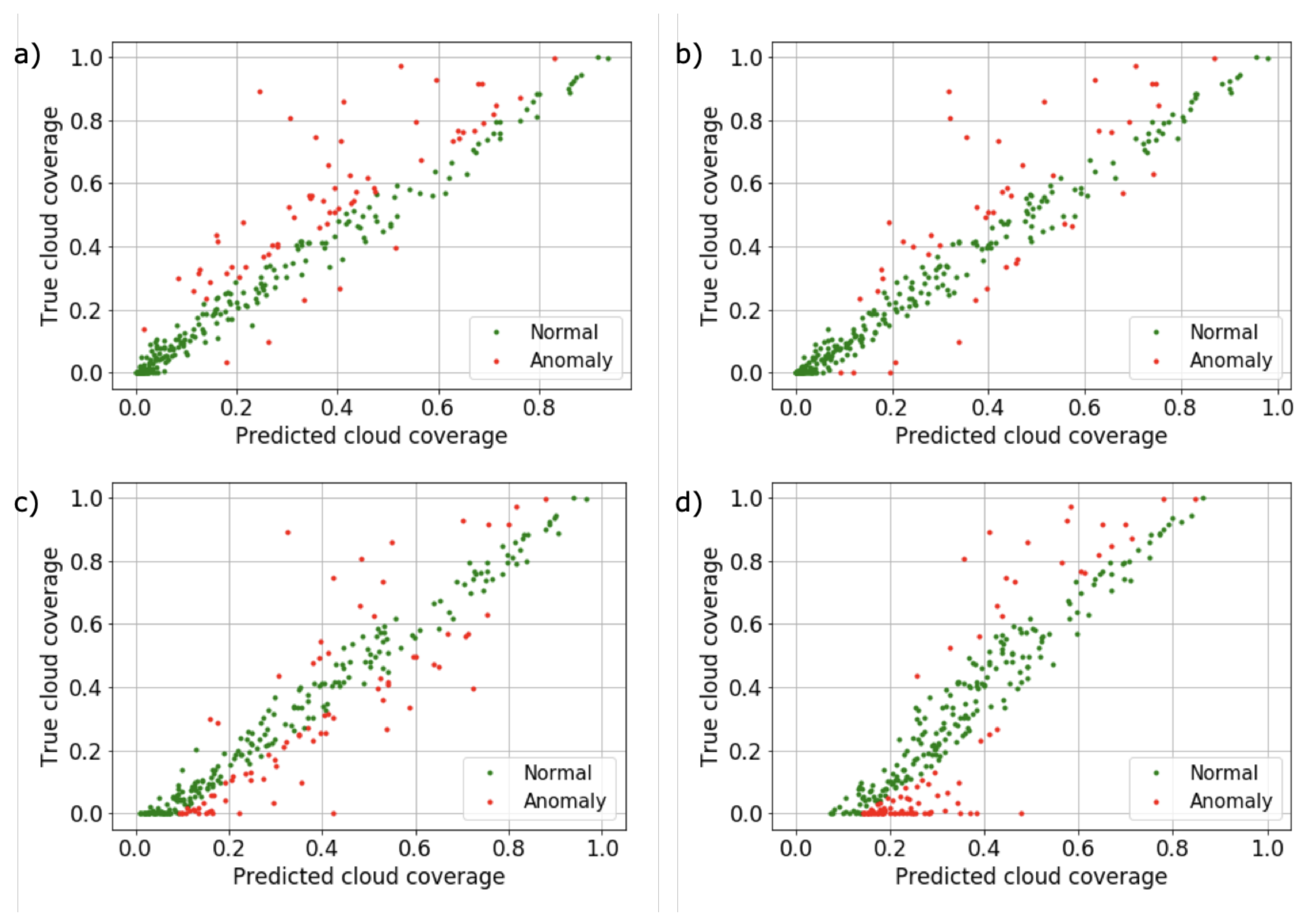
4.1. Effect of Image Resize on Accuracy

Although a label resize method was proposed in Section 3.4.2, residual error due to pixel averaging must be examined. To examine the effect of image resize on accuracy, the priority prediction and cloud coverage prediction results are compared against the original label and the resized label. The comparison results are shown in Figure 9. It can be seen that the overall error is insignificant in achieving the objective. Therefore hereby, resized labels are used as the reference in evaluating the performance throughout the remaining study.

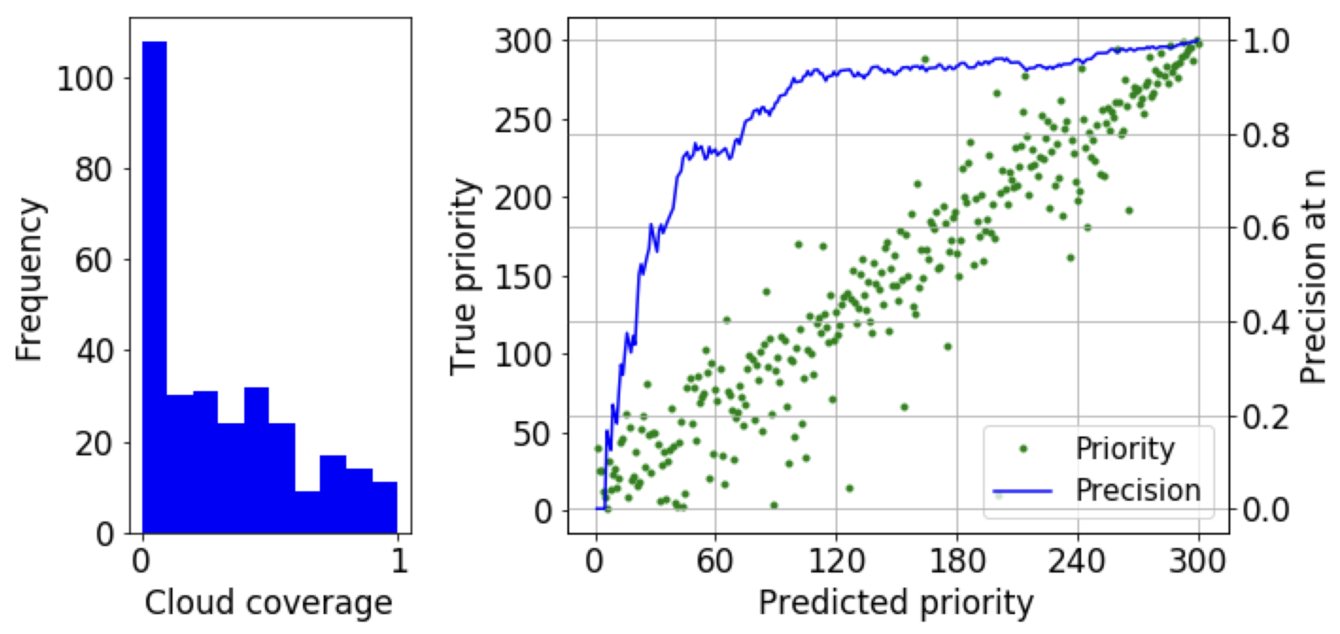
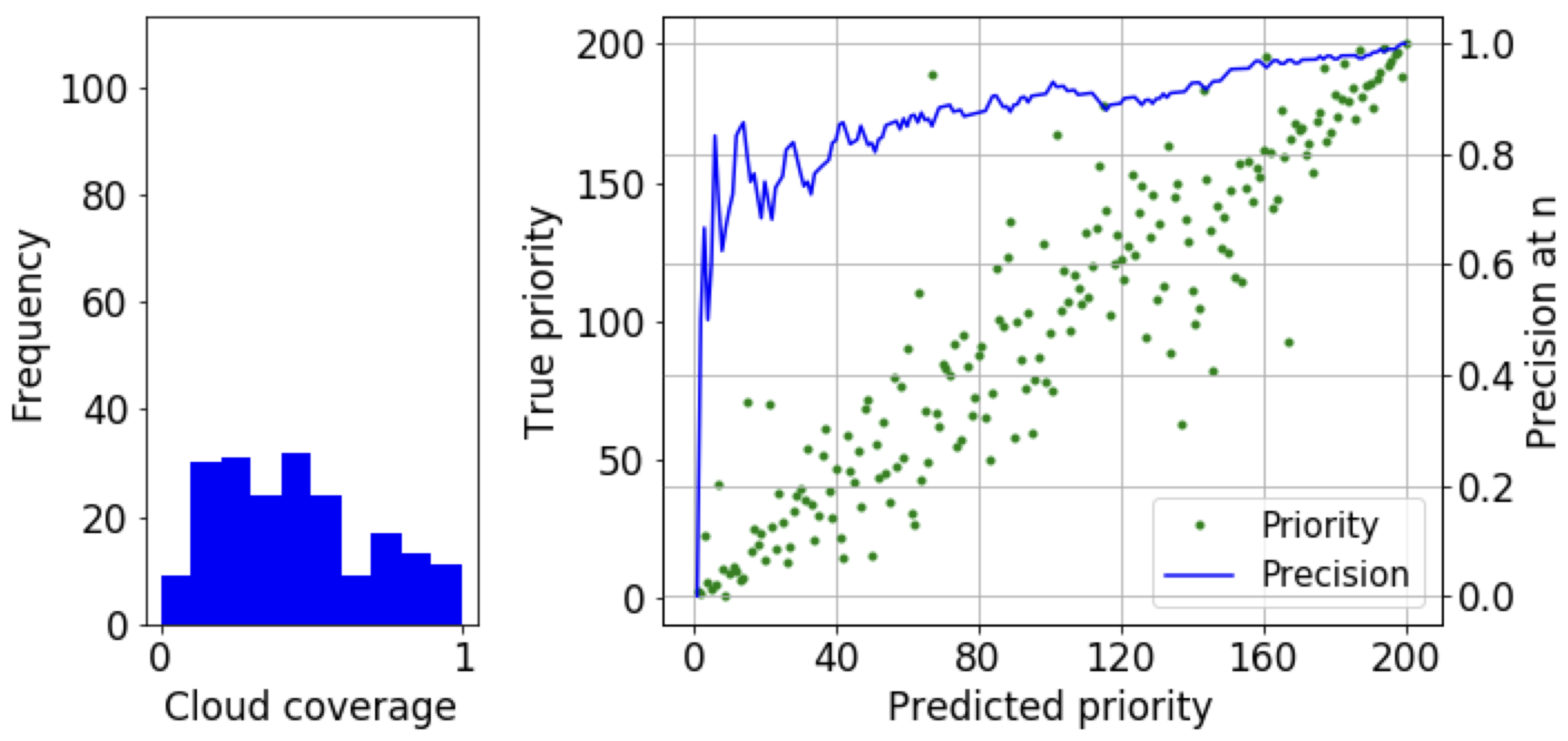
4.2. Effect of Dataset Distribution

As described in Section 3.3, the precision at n will be affected by the distribution of the dataset to be examined. To investigate the effect of the distribution of the dataset, two datasets each with a high and low ratio of clear images were prepared. The results for each of the two datasets are shown in Figure 10 and Figure 11.
The histogram on the left of each figure shows the cloud coverage distribution of the dataset with an interval of 10%. Examining both figures, although it may seem that the performance of the proposed method is low at higher priority images, considering the frequency of the clear images, the practical performance is satisfying. In Figure 10, the number of the top 10% clear images in the dataset is 108, and the precision at 108 is higher than 90%. Considering a downlink capability of 10 images daily, despite the low precision of approximately 10% at 10, all data are clear images. In Figure 11, although the dataset has less clear images in the top 10%, the precision at 10 is approximately 70%. From the results, we can expect the proposed method to be satisfactory also in environments with frequent cloud images [23]. Despite the expectations, the dataset in Figure 10 is used throughout the study to evaluate the proposed method with higher sensitivity.

4.3. Performance Analysis

The performance of the proposed method is compared against RS-Net [29], L-Unet [41], and classical machine learning techniques using RFC (Random Forest Classifier), GBC (Gradient Boosting Classifier), and SVM (Support Vector Machine). RS-Net is selected to compare the performance in terms of precision as it is one of the few methods that consider RGB input while showing high precision results. However, as RS-Net is a heavy network, L-Unet is further selected to compare the performance in inference time as L-Unet is an extremely lightweight network.

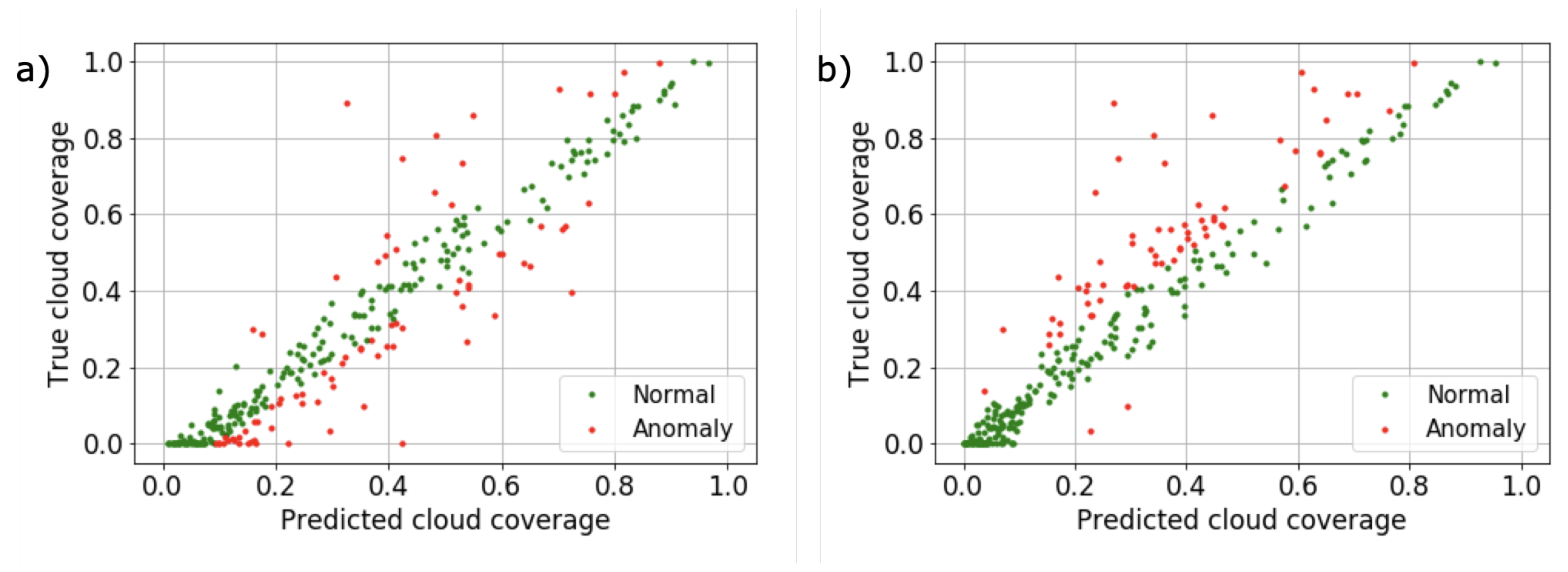
4.3.1. Accuracy and Error Analysis

The prioritization result of the networks is shown in Figure 12. It can be seen that NU-Net without patch decomposition performs almost the same as RS-Net. In the case of NU-Net with patch decomposition, a clear difference in performance can be seen, which comes from the larger border uncertainty described in Section 3.1.2.
Figure 13 shows the segmentation results corresponding to heavily cloudy, lightly cloudy, bright, and city scenes. The green, red, and yellow represent correctly classified cloud (true positive), missed cloud (false negative), and incorrectly classified clear pixels as cloud (true negative), respectively. Only the RFC results are shown out of the classical methods, as random forest had the best results. All methods show reasonably good results in heavily cloudy scenes. The artifacts of border cropping can be seen in the proposed methods (NU1616 and NU4864) and in Jeppesen’s method (RS4864). It can clearly be seen that smaller patches increase the uncertainty, as described in Equation (2) in Section 3.1.2. In the case of lightly cloudy scenes, Zhang’s method shows the best results, particularly over thin clouds. However, Zhang’s method tends to overpredict scenes, including bright features such as a desert or a city. In the bright and city scenes, the proposed method without the patch decomposition (NU4864) shows the best results, followed by Jeppesen’s method (RS4864) and the proposed method with patch decomposition (NU1616).
The characteristics shown in Figure 13 are well represented in Figure 14, in which shows the comparison results of predicted cloud coverage against true cloud coverage. The red dots in Figure 14 represent anomalous data, in which the distance between predicted cloud coverage and true cloud coverage is larger than 1 σ . It can be clearly seen that NU-Net without patch decomposition (Figure 14a) and RS-Net (Figure 14b) have good performance throughout clear images. In contrast, the majority of anomalies are populated in overestimation of clear images in the case of L-Unet (Figure 14d). The NU-Net with patch decomposition (Figure 14c) method slightly overestimates cloud coverage due to the padding effect related to the increase in the border ratio.
Figure 15 shows the anomaly of RS-Net with patch decomposition with and without replication padding applied on the first convolutional block of the network respectively. It can be seen that the overall characteristics share a similar result as RS-Net and NU-Net without patch decomposition when replication padding is not applied. Furthermore, replication padding has a larger effect on small patches, and the padding changes the network characteristics to overestimate cloud coverage. The reason the network characteristics shift to overestimation from underestimation can be explained by comparing zero-padding against unit-padding. In the case of zero-padding the border areas are set to have a non-cloudy boundary, whereas in the case of unit-padding the border areas are set to have a cloudy boundary. As replication padding has been implemented instead of unit-padding, we can expect the boundary condition to be less strict than unit-padding, which keeps the anomalies from departing further away. The reason the padding has a larger effect on the patch decomposition method can be explained by Equation (2), as the padding has a larger impact on the pixels near the border. In this study, since overestimated cloud coverage is preferred as it assures high precision, the replication padding effect can be considered significant. A more complex padding method considering the gradient at the borders of the neighboring patches could further improve the information loss problem near the borders.

4.3.2. Computational Cost Analysis

The computational cost is measured by running the networks on an STMicroelectronics ARM Cortex-M4 based STM32F469BI6NIH6 microcontroller implemented using the X-CUBE-AI package in STM32Cube. HDF5 file is exported from the Keras model [46] of each of the architectures. The X-CUBE-AI package generates a temporary project containing the test code is flashed to the microcontroller. The test code runs the model ten times in batches with random input, and the average runtime of the model is evaluated. In this study, the microcontroller runs at 168 MHz with 2 MB embedded Flash memory and 324 KB embedded RAM when using internal memory and 16 MB NOR Flash and 16 MB SDRAM. The computational cost results are shown in Table 2.
NU-Net without using the patch decomposition, L-Unet, and the proposed method satisfy the design requirement of 13.5 s for inference time to process 6400 images daily. However, NU-Net without patch decomposition requires external memory, whereas the proposed method runs only using embedded memory in the microprocessor, which is a clear advantage for embedded systems if an external component is not required. Although L-Unet has the shortest inference time, performance trade-off exists as shown in Figure 12 and Figure 13. Note that the weights used in the network are floating point. Therefore, the inference time can be further reduced by using quantization [47] methods or using a BNN (Binary Neural Network).

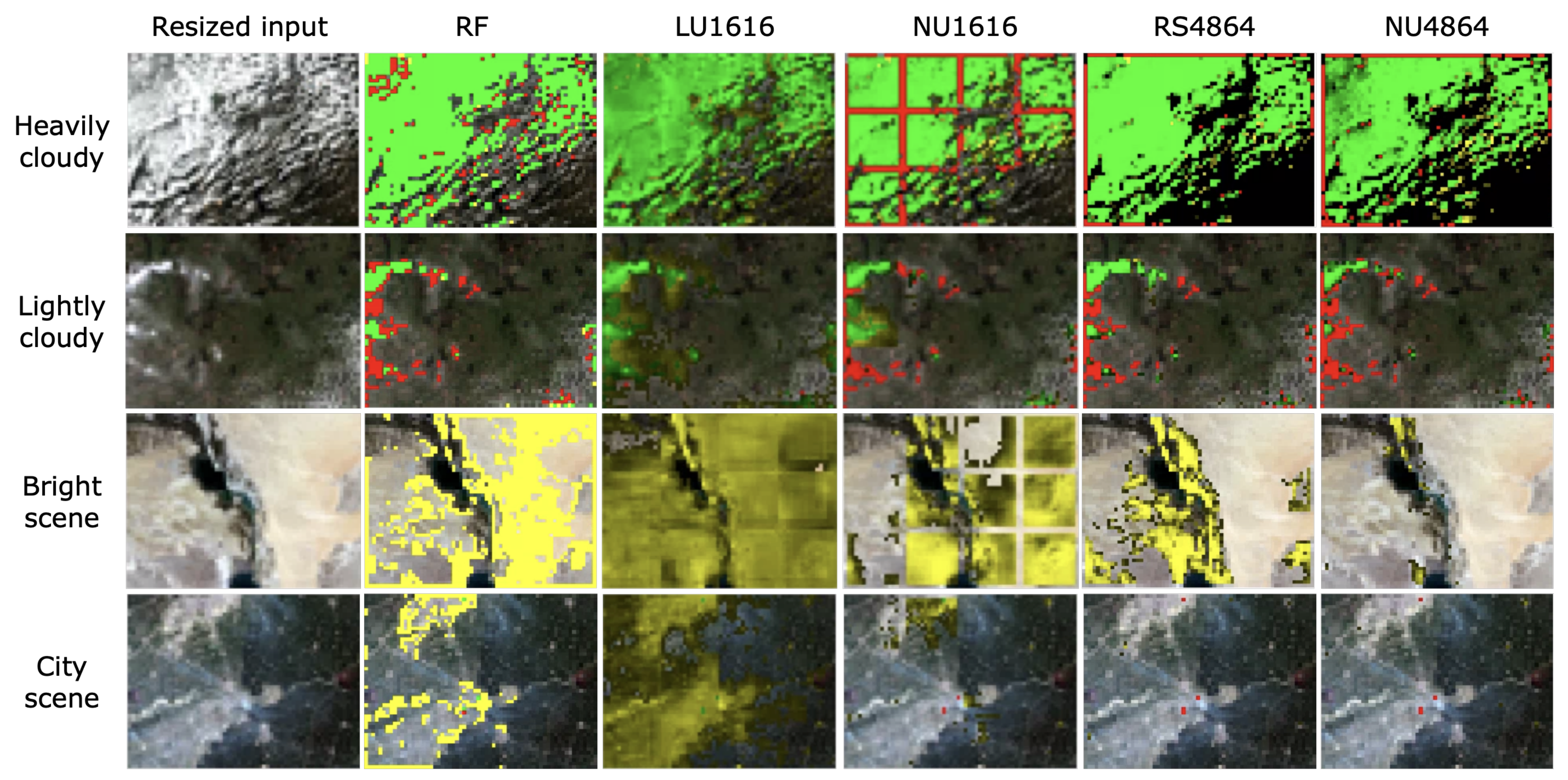
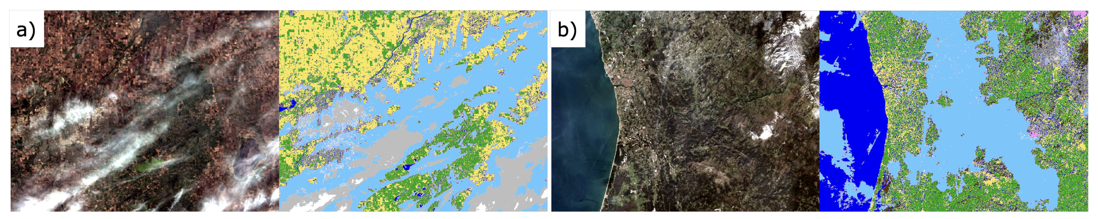
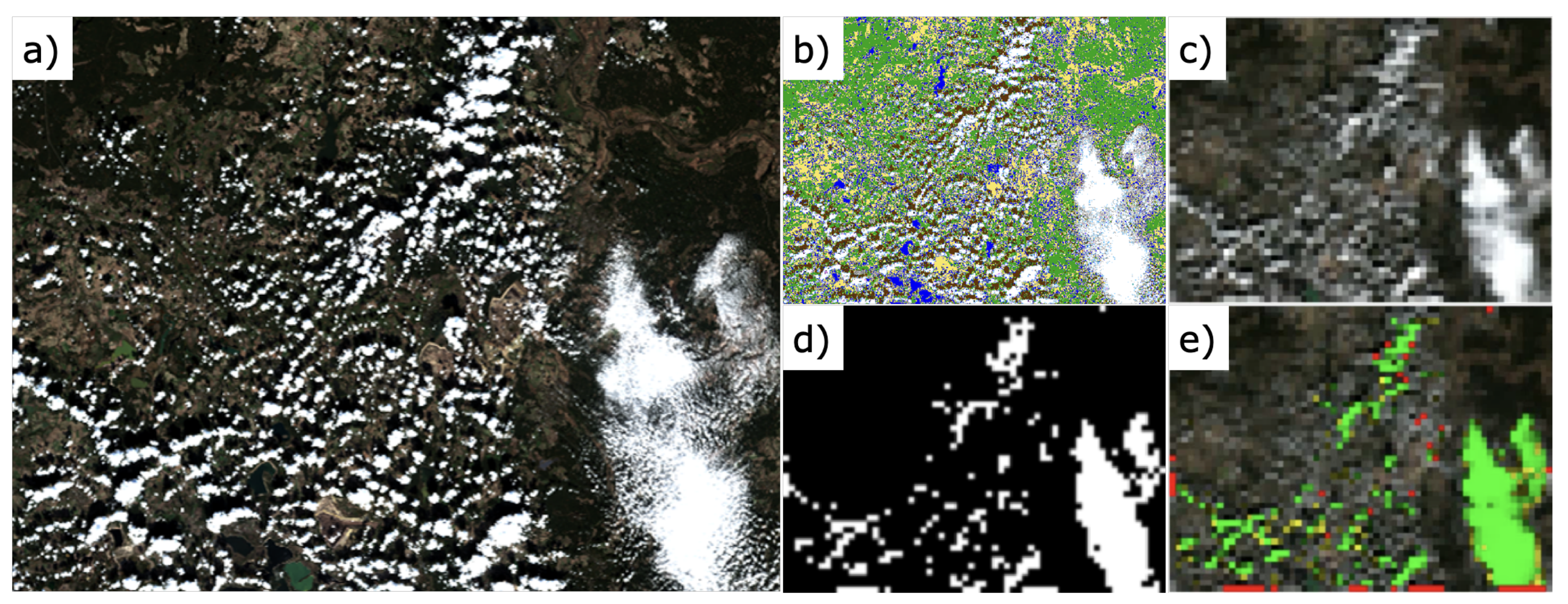
4.4. Visualization of Prioritized Images

Finally, the visualization of the prioritized images using the proposed method is shown in Figure 16. All 300 images from the test dataset were evaluated using NU-Net with the patch decomposition method with a patch size of 16 × 16. High priority scenes are placed on the top left corner with descending order in priority to low priority scenes on the bottom right corner. It can be confirmed from the visualization result that the clear images are prioritized as intended.

5. Limitations of the Proposed Method

In this section, the limitations of the proposed method and corresponding future work related to the limitations of onboard RGB imagers and the effect of input image resizing are discussed in detail.

5.1. Limitation of Onboard RGB Imagers

This study considered only RGB images as the input of the algorithm. Some limitations exist in performing cloud coverage evaluation using such RGB images, especially considering onboard RGB imagers. First, multiple bands have been used in conventional cloud detection methods as previously introduced in Section 2. Various bands play an important role in cloud detection due to the nature of clouds. As the clouds are formed in the atmosphere, the clouds have a similar temperature profile as the well-known atmospheric temperature. Therefore, thermal data can be used to assist cloud detection and further estimate the height of the cloud for evaluating nearby shadows by observing thermal infrared bands. Shortwave infrared bands provide further information in distinguishing cloud with snow/ice, due to the difference in the reflectance of shortwave infrared for cloud from snow/ice. Only using RGB images limit the input information and rely on the CNN to learn deep features such as patterns or texture to classify the clouds. However, deeper features require the CNN architecture to either accompany deeper layers or larger receptive fields, leading to increased computational cost. Other methods, such as augmenting geographical or seasonal information, could provide a mask for non-snow/ice regions.
Secondly, the onboard imagers differ from the visual band data from Landsat or Sentinel, as the pixels in typical CMOS imagers used in nanosatellites are wideband [48]. The wideband channels will inject noise in the proposed method, and therefore will result in performance degradation. A possible solution to these limitations is using a filter wheel with the onboard RGB imagers. Considering that the CMOS imagers have adequate sensitivity in the near-infrared bands, a filter wheel consisting of narrowband green, red, and near-infrared (corresponding to bands 2, 3, and 4) with additional IR cut filter would yield the best results.
Lastly, the inconsistency in the visibility of the cirrus is a source of error when only using RGB images. In this study, cirrus was not masked as cloud due to the inconsistency in the dataset as shown in Figure 17. Cirrus is visible in Figure 17a, whereas cirrus is invisible in Figure 17b. Manual labeling is required to reduce this error, which takes the cost problem in dataset preparation back to the origin.

5.2. Input Image Resize

The input images in the proposed method are scaled down for two main reasons: (1) Reduction in computational time, and (2) to take advantage of dataset generation for post-operational CNN tuning. However, the resizing process averages pixel values with neighboring pixels, resulting in thin or small clouds to blend into clear pixels. Such an effect is larger when the neighboring pixels have dark features, such as cloud shadows. Figure 18 shows an example of the input image resize, resulting in the pixel resolution to degrade from 160 m down to 1600 m. The loss of cloud mask for thin or small clouds can be seen in the resized cloud mask in Figure 18c. These losses result in underestimation of cloud coverage in scenes populated with thin or small clouds. Similarly, cloud shadows are also blended into bright pixels. As cloud shadow is an important feature in validating cloud mask [24,34], resizing results in feature truncation. An ensemble method [49] could be implemented with a dedicated network for detecting small features to improve the proposed method regarding small feature loss.

6. Conclusions

In this research, we have proposed an onboard cloudy image rejection method using machine learning for improving the downlink efficiency of nanosatellites. The main advantage of the proposed method over conventional methods is onboard cloud detection without requiring additional bands. The main strategy was to reduce the input size to reduce the number of arithmetic operations in the CNN. Furthermore, patch decomposition on the input image is introduced to reduce the memory usage when running the CNN. Due to the reduced input size and further patch decomposition, the number of pooling operations was limited to twice. To further cut down the inference time, the number of kernels in the convolution layer was reduced. Finally, a multi-stream architecture was developed to restrain the network from optimizing on simple features such as color. As a result, the proposed method reduced the number of parameters down to 0.4% of RS-Net, while the inference time was reduced down to 4.3% of RS-Net. Considering approximately 67% global cloud fraction [23], we expect the proposed method will enhance the downlink capability of clear images by 112%, assuming 70% precision. Furthermore, the reduced input size helps acquire training images from space for fine tuning, and patch decomposition has potential in parallel cloud coverage estimation in platforms with multicore microprocessors. The in-orbit performance of the proposed method will be evaluated onboard NUcube1, which is scheduled for launch in 2022.

Supplementary Materials

The following are available online at https://www.mdpi.com/2072-4292/12/23/3941/s1, Data D1: Training dataset containing 64 × 48 and 16 × 16 patches, and test dataset containing 640 × 480 images.

Author Contributions

Conceptualization, J.H.P., T.I., R.H., K.O., J.E.K. and K.Y.; methodology, J.H.P., R.H., K.O. and J.E.K.; software, J.H.P.; validation, J.H.P., T.I., R.H., K.O. and J.E.K.; formal analysis, J.H.P., T.I., R.H. and K.O.; investigation, J.H.P., T.I., R.H. and K.O.; resources, T.I. and K.Y.; data curation, J.H.P.; writing—original draft preparation, J.H.P.; writing—review and editing, J.H.P., T.I., R.H., K.O., K.Y. and J.E.K.; visualization, J.H.P.; supervision, T.I., R.H., K.O. and J.E.K.; project administration, T.I.; funding acquisition, K.Y. and T.I. All authors have read and agreed to the published version of the manuscript.

Funding

This research received no external funding.

Acknowledgments

The authors thank Earth Observing System (EOS) for allowing publication using remote sensing images provided through Land Viewer, and the anonymous reviewers for their valuable comments.

Conflicts of Interest

The authors declare no conflict of interest.

Abbreviations

The following abbreviations are used in this manuscript:
ACCAAutomated Cloud-Cover Assessment
AT-ACCAArtificial Thermal Automated Cloud-Cover Assessment
BNNBinary Neural Network
BTBrightness Temperature
CCACloud-Cover Assessment
CNNConvolutional Neural Network
CS-CNNCloud Segmentation CNN
DLASDeep Learning Attitude Sensor
EMEngineering Model
FmaskFunction of mask
FNFalse negative
FOVField of View
FPFalse Positive
GBCGradient Boosting Classifier
HFCNNHierarchical Fusion CNN
IPEXIntelligent Payload Experiment
LDCMLandsat Data Continuity Mission
RFCRandom Forest Classifier
SCLScene Classification map
SLICSimple Linear Iterative Clustering
SPARCSSpatial Procedures for the Automated Removal of Clouds and Shadows
SVMSupport Vector Machine
TCITrue Color Image
TIRSThermal Infrared Sensors
TNTrue negative
TOATop of Atmosphere
TPTrue positive

References

  1. Poghosyan, A.; Golkar, A. CubeSat evolution: Analyzing CubeSat capabilities for conducting science missions. Prog. Aerosp. Sci. 2017, 88, 59–83. [Google Scholar] [CrossRef]
  2. Gill, E.; Sundaramoorthy, P.; Bouwmeester, J.; Zandbergen, B.; Reinhard, R. Formation flying within a constellation of nano-satellites: The QB50 mission. Acta Astronaut. 2013, 82, 110–117. [Google Scholar] [CrossRef] [Green Version]
  3. Butler, D. Many eyes on Earth: Swarms of small satellites set to deliver close to real-time imagery of swathes of the planet. Nature 2014, 505, 143–144. [Google Scholar] [CrossRef] [PubMed]
  4. Devaraj, K.; Kingsbury, R.; Ligon, M.; Breu, J.; Vittaldev, V.; Klofas, B.; Yeon, P.; Colton, K. Dove High Speed Downlink System. In Proceedings of the 31st Annual AIAA/USU Conference on Small Satellites, Logan, UT, USA, 5–10 August 2017. SSC17-VII-02. [Google Scholar]
  5. Planet. Planet Imagery Product Specifications. 2020. Available online: https://www.planet.com/ (accessed on 25 May 2020).
  6. Azami, M.H.; Maeda, G.; Faure, P.; Yamauchi, T.; Kim, S.; Masui, H.; Cho, M. BIRDS-2: A Constellation of Joint Global Multi-Nation 1U CubeSats. J. Phys. Conf. Ser. 1 2019, 1152, 012008. [Google Scholar] [CrossRef]
  7. Park, J.; Jeung, I.-S.; Inamori, T. Telemetry and Two Line Element data analysis for SNUSAT-1b anomaly investigation. In Proceedings of the 32nd International Symposium on Space Technology and Science (ISTS), Fukui, Japan, 15–21 June 2019. 2019-f-76. [Google Scholar]
  8. Malan, D.; Wiid, K.; Burger, H.; Visagie, L. The Development of “nSight-1”—Earth Observation and Science in 2U. In Proceedings of the 31st Annual AIAA/USU Conference on Small Satellites, Logan, UT, USA, 5–10 August 2017. SSC17-X-10. [Google Scholar]
  9. Mas, I.A.; Kitts, C.A. A Flight-Proven 2.4GHz ISM Band COTS Communications System for Small Satellites. In Proceedings of the 21st Annual AIAA/USU Conference on Small Satellites, Logan, UT, USA, 13–16 August 2007. SSC07-XI-11. [Google Scholar]
  10. Evans, D.; Donati, A. The ESA OPS-SAT Mission: Don’t just say there is a better way, fly it and prove it. In Proceedings of the 2018 SpaceOps Conference, Palais du Pharo Marseille, France, 28 May–1 June 2018. [Google Scholar]
  11. Eagleson, S.; Sarda, K.; Mauthe, S.; Tuli, T.; Zee, R. Adaptable, Multi-Mission Design of CanX Nanosatellites. In Proceedings of the 20th Annual AIAA/USU Conference on Small Satellites, Logan, UT, USA, 14–17 August 2006. SSC06-VII-3. [Google Scholar]
  12. Clagett, C.; Santos, L.; Azimi, B.; Cudmore, A.; Marshall, J.; Starin, S.; Sheikh, S.; Zesta, E.; Paschalidis, N.; Johnson, M.; et al. Dellingr: NASA Goddard Space Flight Center’s First 6U Spacecraft. In Proceedings of the 31st Annual AIAA/USU Conference on Small Satellites, Logan, UT, USA, 5–10 August 2017. SSC17-III-06. [Google Scholar]
  13. Klesh, A.; Krajewski, J. MarCO: CubeSats to Mars in 2016. In Proceedings of the 29th Annual AIAA/USU Conference on Small Satellites, Logan, UT, USA, 8–13 August 2015. SSC15-III-3. [Google Scholar]
  14. Kobayashi, M. Iris Deep-Space Transponder for SLS EM-1 CubeSat Missions. In Proceedings of the 31st Annual AIAA/USU Conference on Small Satellites, Logan, UT, USA, 5–10 August 2017. SSC17-II-04. [Google Scholar]
  15. Sako, N. About Nano-JASMINE Satellite System and Project Status. Trans. JSASS Aerosp. Technol. Jpn. 2010, 8, Tf7–Tf12. [Google Scholar] [CrossRef]
  16. Barschke, M.F.; Jonglez, C.; Werner, P.; von Keiser, P.; Gordon, K.; Starke, M.; Lehmann, M. Initial orbit results from the TUBiX20 platform. Acta Astronaut. 2020, 167, 108–116. [Google Scholar] [CrossRef]
  17. Guerra, A.G.; Francisco, F.; Villate, J.; Agelet, F.A.; Bertolami, O.; Rajan, K. On small satellites for oceanography: A survey. Acta Astronaut. 2016, 127, 404–423. [Google Scholar] [CrossRef] [Green Version]
  18. Purivigraipong, S. Review of Satellite-Based AIS for Monitoring Maritime Fisheries. Eng. Trans. 2018, 21, 81–89. [Google Scholar]
  19. Tsuruda, Y.; Aoyanagi, Y.; Tanaka, T.; Matsumoto, T.; Nakasuka, S.; Shirasaka, S.; Matsui, M.; Mase, I. Demonstration of Innovative System Design for Twin Micro-Satellite: Hodoyoshi-3 and -4. Trans. JSASS Aerosp. Technol. Jpn. 2016, 14, Pf131–Pf140. [Google Scholar] [CrossRef] [Green Version]
  20. AlDhafri, S.; AlJaziri, H.; Zowayed, K.; Yun, J.; Park, S. Dubaisat-2 High Resolution Advanced Imaging System (HiRAIS). In Proceedings of the 63rd International Astronautical Congress, Naples, Italy, 1–5 October 2012; Volume 21. IAC-12.B4.6A.6. [Google Scholar]
  21. Bargellini, P.; Emanuelli, P.P.; Provost, D.; Cunningham, R.; Moeller, H. Sentinel-3 Ground Segment: Innovative Approach for future ESA-EUMETSAT Flight Operations cooperation. In Proceedings of the SpaceOps 2010 Conference, Huntsville, Alabama, 25–30 April 2010. AIAA 2010-2193. [Google Scholar]
  22. Mah, G.; O’Brien, M.; Garon, H.; Mott, C.; Ames, A.; Dearth, K. Design and Implementation of the Next Generation Landsat Satellite Communications System. Int. Telemetering Conf. Proc. 2012, 48. Available online: http://hdl.handle.net/10150/581626 (accessed on 21 November 2019).
  23. King, M.; Platnick, S.; Menzel, P.; Ackerman, S.; Hubanks, P. Spatial and Temporal Distribution of Clouds Observed by MODIS Onboard the Terra and Aqua Satellites. IEEE Trans. Geosci. Remote Sens. 2013, 51, 3826–3852. [Google Scholar] [CrossRef]
  24. Zhu, Z.; Woodcock, C.E. Object-based cloud and cloud shadow detection in Landsat imagery. Remote Sens. Environ. 2012, 118, 83–94. [Google Scholar] [CrossRef]
  25. Zhu, Z.; Wang, S.; Woodcock, C.E. Improvement and expansion of the Fmask algorithm: Cloud, cloud shadow, and snow detection for Landsats 4–7, 8, and Sentinel 2 images. Remote Sens. Environ. 2015, 159, 269–277. [Google Scholar] [CrossRef]
  26. Drönner, J.; Korfhage, N.; Egli, S.; Mühling, M.; Thies, B.; Bendix, J.; Freisleben, B.; Seeger, B. Fast Cloud Segmentation Using Convolutional Neural Networks. Remote Sens. 2018, 10, 1782. [Google Scholar] [CrossRef] [Green Version]
  27. Morales, G.; Ramirez, A.; Telles, J. End-to-end Cloud Segmentation in High-Resolution Multispectral Satellite Imagery Using Deep Learning. In Proceedings of the 2019 IEEE XXVI International Conference on Electronics, Electrical Engineering and Computing (INTERCON), Lima, Peru, 12–14 August 2019. [Google Scholar]
  28. Mohajerani, S.; Krammer, T.A.; Saeedi, P. A Cloud Detection Algorithm for Remote Sensing Images Using Fully Convolutional Neural Networks. In Proceedings of the 2018 IEEE 20th International Workshop on Multimedia Signal Processing (MMSP), Vancouver, BC, Canada, 29–31 August 2018; pp. 1–5. [Google Scholar]
  29. Jeppesen, J.H.; Jacobsen, R.H.; Inceoglu, F.; Toftegaard, T.S. A cloud detection algorithm for satellite imagery based on deep learning. Remote Sens. Environ. 2019, 229, 247–259. [Google Scholar] [CrossRef]
  30. Francis, A.; Sidiropoulos, P.; Muller, J.-P. CloudFCN: Accurate and Robust Cloud Detection for Satellite Imagery with Deep Learning. Remote Sens. 2019, 11, 2312. [Google Scholar] [CrossRef] [Green Version]
  31. Irish, R. Landsat 7 Automatic Cloud Cover Assessment. In Algorithms for Multispectral, Hyperspectral, and Ultraspectral Imagery VI; SPIE: Bellingham, WA, USA, 2000; Volume 4049, pp. 348–355. [Google Scholar]
  32. Irish, R.; Barker, J.; Goward, S.; Arvidson, T. Characterization of the Landsat-7 ETM+ Automated Cloud-Cover Assessment (ACCA) algorithm. Photogammetric Eng. Remote. Sens. 2006, 72, 1179–1188. [Google Scholar] [CrossRef]
  33. Scaramuzza, P.L.; Bouchard, M.A.; Dwyer, J.L. Development of the Landsat Data Continuity Mission Cloud-Cover Assessment Algorithms. IEEE Trans. Geosci. Remote Sens. 2012, 50, 1140–1154. [Google Scholar] [CrossRef]
  34. Goodwin, N.R.; Collett, L.J.; Denham, R.J.; Flood, N.; Tindall, D. Cloud and cloud shadow screening across Queensland, Australia: An automated method for Landsat TM/ETM + time series. Remote Sens. Environ. 2013, 134, 50–65. [Google Scholar] [CrossRef]
  35. Hughes, M.J.; Hayes, D.J. Automated Detection of Cloud and Cloud Shadow in Single-Date Landsat Imagery Using Neural Networks and Spatial Post-Processing. Remote Sens. 2014, 6, 4907–4926. [Google Scholar] [CrossRef] [Green Version]
  36. Wei, J.; Huang, W.; Li, Z.; Sun, L.; Zhu, X.; Yuan, Q.; Liu, L.; Cribb, M. Cloud detection for Landsat imagery by combining the random forest and superpixels extracted via energy-driven sampling segmentation approaches. Remote Sens. Environ. 2020, 248, 112005. [Google Scholar] [CrossRef]
  37. Yamashita, R.; Nishio, M.; Do, R.K.G.; Togashi, K. Convolutional neural networks: An overview and application in radiology. Insights Imaging 2018, 9, 611–629. [Google Scholar] [CrossRef] [PubMed] [Green Version]
  38. Shi, M.; Xie, F.; Zi, Y.; Yin, J. Cloud Detection of Remote Sensing Images by Deep Learning. In Proceedings of the 2016 IEEE International Geoscience and Remote Sensing Symposium (IGARSS), Beijing, China, 10–15 July 2016; pp. 701–704. [Google Scholar]
  39. Liu, H.; Zeng, D.; Tian, Q. Super-Pixel Cloud Detection Using Hierarchical Fusion CNN. In Proceedings of the 2018 IEEE Fourth International Conference on Multimedia Big Data (BigMM), Xi’an, China, 13–16 September 2018. [Google Scholar]
  40. Achanta, R.; Shaji, A.; Smith, K.; Lucchi, A.; Fua, P.; Süsstrunk, S. SLIC Superpixels Compared to State-of-the-Art Superpixel Methods. IEEE Trans. Pattern Anal. Mach. Intell. 2012, 34, 2274–2281. [Google Scholar] [CrossRef] [PubMed] [Green Version]
  41. Zhang, Z.; Iwasaki, A.; Xu, G.; Song, J. Cloud detection on small satellites based on lightweight U-net and image compression. J. Appl. Remote Sens. 2019, 13, 026502. [Google Scholar] [CrossRef]
  42. Ronneberger, O.; Fischer, P.; Brox, T. U-Net: Convolutional Networks for Biomedical Image Segmentation. arXiv 2015, arXiv:1505.04597v1. [Google Scholar]
  43. Craswell, N. Precision at n. In Encyclopedia of Database Systems; Springer: Boston, MA, USA, 2009. [Google Scholar]
  44. Louis, J.; Debaecker, V.; Pflug, B.; Main-Knorn, M.; Bieniarz, J.; Mueller-Wilm, U.; Cadau, E.; Gascon, F. Sentinel-2 Sen2Cor: L2A Processor for Users. In Proceedings of the Living Planet Symposium 2016; ESA Communications: Noordwijk, The Netherlands, 2016; ESA SP-740. [Google Scholar]
  45. Gascon, F.; Bouzinac, C.; Thépaut, O.; Jung, M.; Francesconi, B.; Louis, J.; Lonjou, V.; Lafrance, B.; Massera, S.; Gaudel-Vacaresse, A.; et al. Copernicus Sentinel-2A Calibration and Products Validation Status. Remote Sens. 2017, 9, 584. [Google Scholar] [CrossRef] [Green Version]
  46. Chollet, F. Keras. 2015. Available online: https://keras.io (accessed on 21 November 2019).
  47. Cheng, J.; Wu, J.; Leng, C.; Wang, Y.; Hu, Q. Quantized CNN: A Unified Approach to Accelerate and Compress Convolutional Networks. IEEE Trans. Neural Netw. Learn. Syst. 2018, 29, 4730–4743. [Google Scholar] [CrossRef]
  48. Maskey, A. Imaging Payload System Design for Nano-Satellite Applications in Low-Earth Orbit. Master’s Thesis, Seoul National University, Seoul, Korea, 2016. [Google Scholar]
  49. Hamaguchi, R.; Hikosaka, S. Building Detection from Satellite Imagery using Ensemble of Size-specific Detectors. In Proceedings of the 2018 IEEE/CVF Conference on Computer Vision and Pattern Recognition Workshops (CVPRW), Salt Lake City, UT, USA, 18–22 June 2018; pp. 223–227. [Google Scholar]
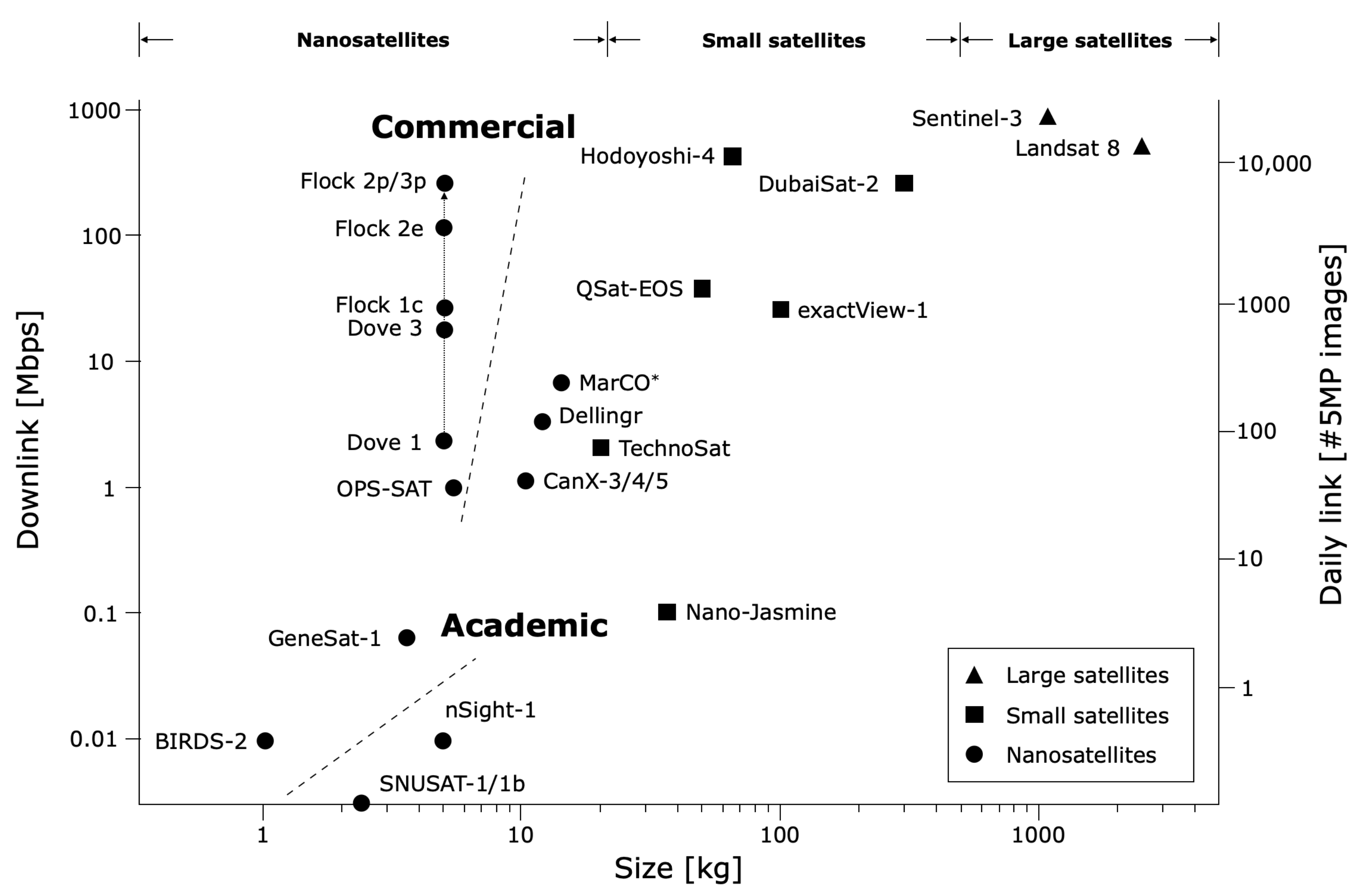
Figure 1. Downlink capability of various spacecrafts. Nanosatellites are limited in downlink data, therefore being able to downlink high priority data is more important compared to larger satellites that have the capability of bulk downlink. The class and downlink information (band, RF power, and downlink throughput) and corresponding references for each satellite are shown in Table 1.
Remotesensing 12 03941 g001
Figure 2. Overview of the flowchart of the proposed method. Each part in (a) image resize, (b) patch decomposition, (c) cloud coverage prediction, and (d) cloud coverage fraction evaluation are designed to reduce inference time.
Remotesensing 12 03941 g002
Figure 3. An example of patch decomposition with 16 × 16 × 3 patch and a 16 × 16 stride on a 64 × 48 × 3 image. The patch decomposition results in 12 patches as shown on the right-hand side of the figure.
Remotesensing 12 03941 g003
Figure 4. Variations of the paddings around the border used in the convolutional layer of the CNN: (a) zero padding, (b) reflection padding, and (c) replication padding. The red box shows the boundary at the top left-hand corner of an image, and the numbers in each pixel represent the pixel value.
Remotesensing 12 03941 g004
Figure 5. Schematic of NU-Net architecture proposed in this study. NU-Net is a modified lightweight version of RS-Net with multi-stream architecture in order to suppress the network from optimizing in color features.
Remotesensing 12 03941 g005
Figure 6. Precision at n used as an accuracy metric in the study. Precision is chosen as the specific accuracy metric as the main objective is to prevent downlink of cloudy images. The figure shows an evaluation example of precision at 0.4 .
Remotesensing 12 03941 g006
Figure 7. Overview of automatic dataset generation using Sentinel-2 products. RGB and SCL data are paired to ensure the extracted mask from SCL corresponds to the same area over RGB. (a) RGB and SCL data are prepared and (b) cropped to an arbitrary input image size. (c) Patches are extracted over the same area, and (d) the target feature masks are generated based on the SCL data.
Remotesensing 12 03941 g007
Figure 8. Label resize for scaling down the size of the label. Thin cirrus, high probability cloud, and medium probability cloud features are remapped to red, green, and blue channels. Channel-wise feature decomposition gives a higher degree of freedom in averaging methods upon downsampling.
Remotesensing 12 03941 g008
Figure 9. (a) Priority and (b) cloud coverage prediction results compared against labels before and after resize. The results show a similar trend between before and after resize, which indicates the resize method can be considered valid.
Remotesensing 12 03941 g009
Figure 10. Prioritization result for clear image rich dataset. Spearman’s rank correlation coefficient ρ = 0.946 .
Remotesensing 12 03941 g010
Figure 11. Prioritization result for balanced dataset. Spearman’s rank correlation coefficient ρ = 0.977 .
Remotesensing 12 03941 g011
Figure 12. Precision at n for NU-Net (proposed), RS-Net (Jeppesen, 2019), without patch decomposition, and NU-Net (proposed) and L-Unet (Zhang, 2019) with patch decomposition. CNN methods are also compared with classical methods using RF, GBC, and SVM. Spearman’s rank correlation coefficient is ρ N U 4864 = 0.962, ρ R S 4864 = 0.961, ρ R S 1616 = 0.946, ρ L U 1616 = 0.837, ρ R F 4864 = 0.903, ρ G B C 4864 = 0.890, and ρ S V M 4864 = 0.795 respectively.
Remotesensing 12 03941 g012
Figure 13. Selected segmentation results for heavily cloudy, lightly cloudy, bright, and city scenes (RF: Random Forest, LU1616: Zhang’s method, NU1616: Proposed method with patch decomposition, RS4864: Jeppesen’s method, NU4864: Proposed method without patch decomposition). Green, red, and yellow represent true positive, false negative, and true negative, respectively.
Remotesensing 12 03941 g013
Figure 14. Cloud coverage prediction error depending on CNN models with anomaly points for error distances larger than 1 σ . (a) NU-Net (proposed) without patch decomposition, (b) RS-Net (Jeppesen, 2019) without patch decomposition, (c) NU-Net (proposed) with 16×16 patch decomposition, and (d) L-Unet (Zhang, 2019) with 16×16 patch decomposition.
Remotesensing 12 03941 g014
Figure 15. Effect of reflection padding in the first convolutional block on cloud coverage, (a) with reflection padding and (b) without reflection padding applied on the first block. Reflection padding changes the network characteristics to overestimate cloud coverage, which has a positive effect in performance regarding precision.
Remotesensing 12 03941 g015
Figure 16. Visualization of image prioritization using NU-Net with patch decomposition of 16 × 16 patch. The images with the highest priority have been aligned from the top left corner down to the bottom right corner.
Remotesensing 12 03941 g016
Figure 17. When only the RGB image is used, (a) cirrus in Sentinel-2 SCL data may sometimes be visible as shown on the left and (b) sometimes invisible as shown on the right. In this study, cirrus is neglected and is considered as a noise source.
Remotesensing 12 03941 g017
Figure 18. The effect of input image resize. Thin or small features are blended into neighboring pixels, resulting in underestimating cloud coverage in scenes with high populations of thin or small clouds. The figure shows an example of (a) original input image, (b) SCL, (c) resized image, (d) resized cloud mask, and (e) cloud coverage estimation result, respectively. The losses in small clouds can be seen in the resized image and mask.
Remotesensing 12 03941 g018
Table 1. Detailed information on the downlink capacity of various spacecrafts for Figure 1. (* Maximum achieved in laboratory tests).
SatelliteClassMassRF InformationReference
BandRF PowerThroughput
Birds-2Nanosatellite1 kg (1U)UHF0.8 W9.6 kbps [6]
SNUSAT-1bNanosatellite1.9 kg (2U)UHF0.5 W1.2 kbps [7]
nSight-1Nanosatellite5 kg (2U)UHF-9.6 kbps [8]
GeneSat-1Nanosatellite3.5 kgS-band-83 kbps [9]
OPS-SATNanosatellite5.4 kg (3U)S-band-1 Mbps [10]
CanX-3/4/5Nanosatellite10 kgS-band-1 Mbps [11]
DellingrNanosatellite11 kgUHF2 W3 Mbps [12]
MarCONanosatellite13.5 kg (6U)X-band4 W6.25 Mbps * [13,14]
Dove 1Nanosatellite5 kg (3U)X-band2 W4 Mbps [4]
Dove 3Nanosatellite5 kg (3U)X-band2 W25 Mbps [4]
Flock 1cNanosatellite5 kg (3U)X-band2 W34 Mbps [4]
Flock 2eNanosatellite5 kg (3U)X-band2 W100 Mbps [4]
Flock 2p/3pNanosatellite5 kg (3U)X-band2 W220 Mbps [4]
Nano-JasmineSmall satellite35 kgS-band-100 kbps [15]
TechnoSatSmall satellite20 kgS-band0.5 W1.39 Mbps[16]
QSat-EOSSmall satellite50 kgKu-band-30 Mbps[17]
exactView-1Small satellite100 kgC-band5 W20 Mbps[18]
Hodoyoshi-4Small satellite64 kgX-band2 W350 Mbps[19]
DubaiSat-2Small satellite300 kgX-band-160 Mbps[20]
Sentinel-3Large satellite1150 kgX-band-520 Mbps[21]
Landsat-8Large satellite2623 kgX-band50 W384 Mbps[22]
Table 2. Computational cost results for selected models. Inference time is only for CNN excluding image pre-processing time. ( 1 External memory used, 2 Inference time for 12 patches).
NetworkResource UsageInference Time
(ms)
Precision
at 60
ModelImagePatchParametersROM (KB)RAM (KB)
Jeppesen, 201948 × 6448 × 647,854,59230,666.50 1 2304.00 1 58,723.4380.867
Proposed48 × 6448 × 6429,907115.83 1 864.00 1 4886.6740.900
Zhang, 201948 × 6416 × 16982837.3896.00987.12 2 0.583
Proposed48 × 6416 × 1629,907127.3372.002499.84 2 0.767
Sample Availability: The dataset and codes for reproducing the work presented in this study are available from the authors.
Publisher’s Note: MDPI stays neutral with regard to jurisdictional claims in published maps and institutional affiliations.

