Combined Effects of Impervious Surface Change and Large-Scale Afforestation on the Surface Urban Heat Island Intensity of Beijing, China Based on Remote Sensing Analysis

Abstract

Urban heat island (UHI) attenuation is an essential aspect for maintaining environmental sustainability at a local, regional, and global scale. Although impervious surfaces (IS) and green spaces have been confirmed to have a dominant effect on the spatial differentiation of the urban land surface temperature (LST), comprehensive temporal and quantitative analysis of their combined effects on LST and surface urban heat island intensity (SUHII) changes is still partly lacking. This study took the plain area of Beijing, China as an example. Here, rapid urbanization and a large-scale afforestation project have caused distinct IS and vegetation cover changes within a small range of years. Based on 8 scenes of Landsat 5 TM/7ETM/8OLI images (30 m × 30 m spatial resolution), 920 scenes of EOS-Aqua-MODIS LST images (1 km × 1 km spatial resolution), and other data/information collected by different approaches, this study characterized the interrelationship of the impervious surface area (ISA) dynamic, forest cover increase, and LST and SUHII changes in Beijing’s plain area during 2009–2018. An innovative controlled regression analysis and scenario prediction method was used to identify the contribution of ISA change and afforestation to SUHII changes. The results showed that percent ISA and forest cover increased by 6.6 and 10.0, respectively, during 2009–2018. SUHIIs had significant rising tendencies during the decade, according to the time division of warm season days (summer days included) and cold season nights (winter nights included). LST changes during warm season days responded positively to a regionalized ISA increase and negatively to a regionalized forest cover increase. However, during cold season nights, LST changes responded negatively to a slight regionalized ISA increase, but positively to an extensive regionalized ISA increase, and LST variations responded negatively to a regionalized forest cover increase. The effect of vegetation cooling was weaker than ISA warming on warm season days, but the effect of vegetation cooling was similar to that of ISA during cold season nights. When it was assumed that LST variations were only caused by the combined effects of ISA changes and the planting project, it was found that 82.9% of the SUHII rise on warm season days (and 73.6% on summer days) was induced by the planting project, while 80.6% of the SUHII increase during cold season nights (and 78.9% during winter nights) was caused by ISA change. The study presents novel insights on UHI alleviation concerning IS and green space planning, e.g., the importance of the joint planning of IS and green spaces, season-oriented UHI mitigation, and considering the thresholds of regional IS expansion in relation to LST changes.

1. Introduction

The urban heat island (UHI) effect occurs when urban areas have higher temperatures than surrounding rural areas [1], which can contribute to a series of environmental and socio-economic problems, e.g., increasing the frequency and persistence of heat waves [2,3], raising energy consumption [4], accelerating air pollution [5], and threatening public health [6]. In the current context of global climate change and rapid urbanization, UHI attenuation based on a better understanding of its influential factors and mechanisms is a pressing issue for sustainable development [7].

UHI can be measured via both the atmospheric and land surface temperature. The latter, in terms of surface UHI (SUHI), has been studied more frequently due to the advantage of data acquisition through remote sensing imageries [8]. Urban land surface characteristics (e.g., albedo, emissivity, and thermal capacity) that are mostly determined by land-use/land-cover (LULC) varieties have been found to have a major impact on the SUHI [9]. Accordingly, a number of studies have focused on discovering the contributions of both the LULC composition and configuration to the land surface temperature (LST). Commonly, on hot summer days, impervious surfaces (IS) increase LST by raising sensible heat flux, whereas green spaces (especially forests) lower the ambient air temperature through reducing the absorption of solar radiance and increasing latent heat flux [10,11]. Water bodies also have negative effects on LST due to their high heat capacity and evaporative cooling [12]. Additionally, the effects of the LULC configuration on LST variations have been confirmed, e.g., clustered impervious surfaces/vegetation cover act more strongly in elevating/lowering LST [13], and the rational use of connectivity from a landscape source–sink point of view can bring additional cooling effects [14]. On the whole, the composition of LULC has been proven to be more important in influencing LST than the configuration based on macro-scale remote sensing observations, and the proportions of impervious surface (IS) and green spaces have been shown to have a dominant effect on LST spatial differentiation in different seasons [15,16,17,18,19,20,21].

Compared with the pattern analysis of LST in relation to the LULC composition and configuration, the temporal dynamic of LST in response to LULC conversions seems to be more complicated and has been given less attention. Yu et al. [22] explored summertime LST changes in an urban agglomeration of southern China. Their study concluded that the transformation of built-up areas from all other land cover types can increase LST, except for bare land, and the transformation of forestland from all other land cover types decreases LST. Akinvemi et al. [23] and Muro et al. [24] studied land cover variations of dryland and wetland regions in relation to LST changes, respectively, also concluding that positive LST trends corresponded to deforestation and farmland expansion, while negative LST trends corresponded to forestation processes. In addition to studies following the land use transfer matrix, research has looked into the relationships between individual LULC component (especially IS and vegetation cover) dynamics and LST changes. For example, time-series models were used to measure and predict LST changes in relation to urban expansion [25,26,27,28]. It is anticipated that urban expansion-induced global warming between 2015 and 2050 will be about half to two times as strong as that caused by greenhouse gas emissions [29]. Vegetation cooling has been valued as a nature-based solution (NBS) for counteracting the negative effects of urbanization [30,31,32]. However, the effects of IS and vegetation cover changes of the same area in influencing LST are inequivalent, as IS change generally has a stronger relationship with LST [33,34,35]. Moreover, the cooling/warming effect and magnitude of vegetation gain/loss are still debated, as few studies have found that they highly depend on the growing stages, previous land cover types, and biophysical characteristics [22,36,37,38].

The SUHI intensity (SUHII) reflects the UHI effect directly and quantitatively. So far, three types of methods have been applied to estimate SUHII: LST as a proxy of SUHI; the LST difference between the urban and reference areas; and non-parametric models [39,40]. While the second method is the most commonly used, the third of non-parametric models can avoid the problem of defining urban–rural boundaries that cause additional SUHII deviations [41,42,43]. Research on the temporal dynamic analysis of SUHII in response to LULC changes has been very limited. Li et al. [44] studied approximately 5000 urban areas of the conterminous United States and showed that the urban area size alone can explain as much as 87% of the variance of SUHII during urban expansion. Yao et al. [45] found that rural greening contributed to 22.5% of the increased daytime SUHII in the growing season at a global scale during 2001–2017, indicating that afforestation or reforestation could also exacerbate the UHI effect without rational spatial planning. Overall, despite the high-ranking importance of IS and vegetation cover changes in influencing urban LST having been demonstrated, their effects on SUHII changes remain largely unknown.

In general, past research has provided plentiful references for urban landscape planning in terms of coping with the UHI effect, especially IS and green spaces at a local scale. As shown by Zhou et al. [39,40], SUHII publications have grown exponentially since 2005 due to the growing interest associated with rapid urbanization and global warming, in addition to the advancement of new remote sensing techniques. However, with respect to these pieces of literature, debate exists, for example, on aspects of the cooling effects of afforestation or reforestation, as well as their role in SUHII attenuation. Moreover, although the changing trend of LST in response to LULC conversions has been frequently discussed, quantitative relationships are still unclear due to inadequate time-series analysis. Furthermore, many relevant studies have focused on a specific time (generally summer), whereas inter-annual variations of LST changes in response to LULC conversions are yet to be explored in seasonal and diurnal divisions. Additionally, focus on practically implemented urban strategies could refresh the conclusions of this field of study, especially if advanced remote sensing techniques were applied [46]. It is therefore important to follow opportunities that could motivate new insights on this “old” topic.

Due to rapid development, some Chinese megacities (e.g., Beijing) have seen extensive IS expansion and greening efforts during the past two or three decades [47]. From 2012 to 2015, the Beijing municipal government accomplished a large-scale planting project to increase forest cover by over 10% in its plain area—the One-Million-Mu (666 km²) Plain Afforestation Project [48]. This unprecedented greening project motivated the conception of this study, leading to three specific questions: (a) How have IS, forest cover, and LST changed over the range of years covering the large-scale afforestation period in the plain area of Beijing?; (b) what is the interrelationship among IS, forest cover, and LST changes with seasonal and diurnal variations?; and (c) how have IS change and afforestation influenced the SUHIIs of this area? Based on remote sensing data of Landsat 5 TM/7ETM/8OLI images (30 m × 30 m spatial resolution), EOS-Aqua-MODIS LST images (1 km × 1 km spatial resolution), and other data/information collected from different approaches, a series of methods, including temporal trend analysis, regression analysis, and a new technique of scenario prediction, were used to find answers to the three questions. The study aimed to provide implications for sustainable urban landscape planning in coping with UHI, based on a novel understanding of the combined effects of IS and forest cover changes on LST and SUHII variations.

2. Materials and Methods

2.1. Study Area

Beijing covers an area of 16,410 km². It has a warm temperate and monsoon-influenced continental climate, with hot humid summers and cold, windy, and dry winters. The Taihang and Yanshan Mountains shield the city to the north, northwest, and west, while the North China Plain opens to the south and east of the city (Figure 1b). The plain area (6338 km², altitude generally lower than 100 m) hosts the majority of the population of Beijing and has experienced drastic urban expansion driven by concentric development, with the appearance of five city ring roads (Figure 1c) [49,50]. A negative influence of urban expansion on the thermal environment of Beijing has been found [51,52]. From 1960 to 2008, the annual mean temperature of Beijing increased 0.39 °C per year on average, which is much higher than the global warming rate of 0.13 °C [53]. A previous study also revealed that latent heat flux (LHF) in the plain areas changed more drastically from 1997 to 2017 compared with the mountain areas [51].

2.2. Data Collection and Preprocessing

2.2.1. Extraction of the Impervious Surface Area (ISA)

Standard terrain corrected (L1T) Landsat 5 TM, 7 ETM+, and 8 OLI/TIRS imagery (30 m × 30 m spatial resolution) acquired on 09-22-2009, 07-26-2011, 09-04-2014, and 07-10-2017 was used to extract the ISA in Beijing’s plain area at different stages during the decade of 2009–2018. Each imaging day had two scenes that covered the study area and their path/row was 123/32 and 123/33. All images were downloaded from the United States Geological Survey (USGS) website (https://earthexplorer.usgs.gov/).

Image preprocessing was conducted with the ENVI software (version 5.2; Exelis VIS, Inc., Boulder, CO, USA). Procedures included radiometric correction, FLASH atmospheric correction, image mosaicing, and image cutting. The Modified Normalized Difference Water Index (MNDWI) was calculated following Equation (1) [54], in order to extract water cover by exploring and setting threshold values.

$$\mathrm{MNDWI}=\frac{\mathrm{GREEN}-\mathrm{SWIR}}{\mathrm{GREEN}+\mathrm{SWIR}},$$

(1)

where GREEN and SWIR represent the reflectance of green (band 2 of Landsat 5 TM and 7 ETM+, and band 3 of Landsat 8 OLI/TIRS) and shortwave infrared (SWIR 1, band 5 of Landsat 5 TM and 7 ETM+, and band 6 of Landsat 8 OLI/TIRS) spectral bands, respectively.

Furthermore, the Biophysical Composition Index (BCI) was calculated to extract ISA by exploring and setting threshold values. BCI was proposed by Deng and Wu [55] following Ridd’s [56] conceptual vegetation-impervious surface-soil triangle model, and was derived by reexamining the components of Tasseled Cap (TC) transformation using Equation (2):

$$\mathrm{BCI}=\frac{\left(\mathrm{H}+\mathrm{L}\right)/2-\mathrm{V}}{\left(\mathrm{H}+\mathrm{L}\right)/2+\mathrm{V}},$$

(2)

where H is “high albedo”, the normalized TC1; L is “low albedo”, the normalized TC3; and V is “vegetation”, the normalized TC2. These three factors can be calculated as follows:

$$\mathrm{H}=\frac{\mathrm{TC}1-\mathrm{TC}{1}_{\min }}{\mathrm{TC}{1}_{\max }-\mathrm{TC}{1}_{\min }},$$

(3)

$$\mathrm{L}=\frac{TC3-TC{3}_{min}}{TC{3}_{max}-TC{3}_{min}},$$

(4)

$$\mathrm{V}=\frac{TC2-TC{2}_{min}}{TC{2}_{max}-TC{2}_{min}},$$

(5)

where TCi (i = 1, 2, and 3) represents the first three TC components, and TCi_min and TCi_max are the minimum and maximum values of the ith TC component, respectively. TC transformation of Landsat 5 TM and Landsat 7 ETM+ images was realized using the default parameters in ENVI 5.2, while TC transformation of Landsat 8 OLI/TIRS images was conducted following the study of Baig et al. [57].

Finally, 300 checking points were randomly selected to testify the classification results in reference to high-resolution Google Earth images.

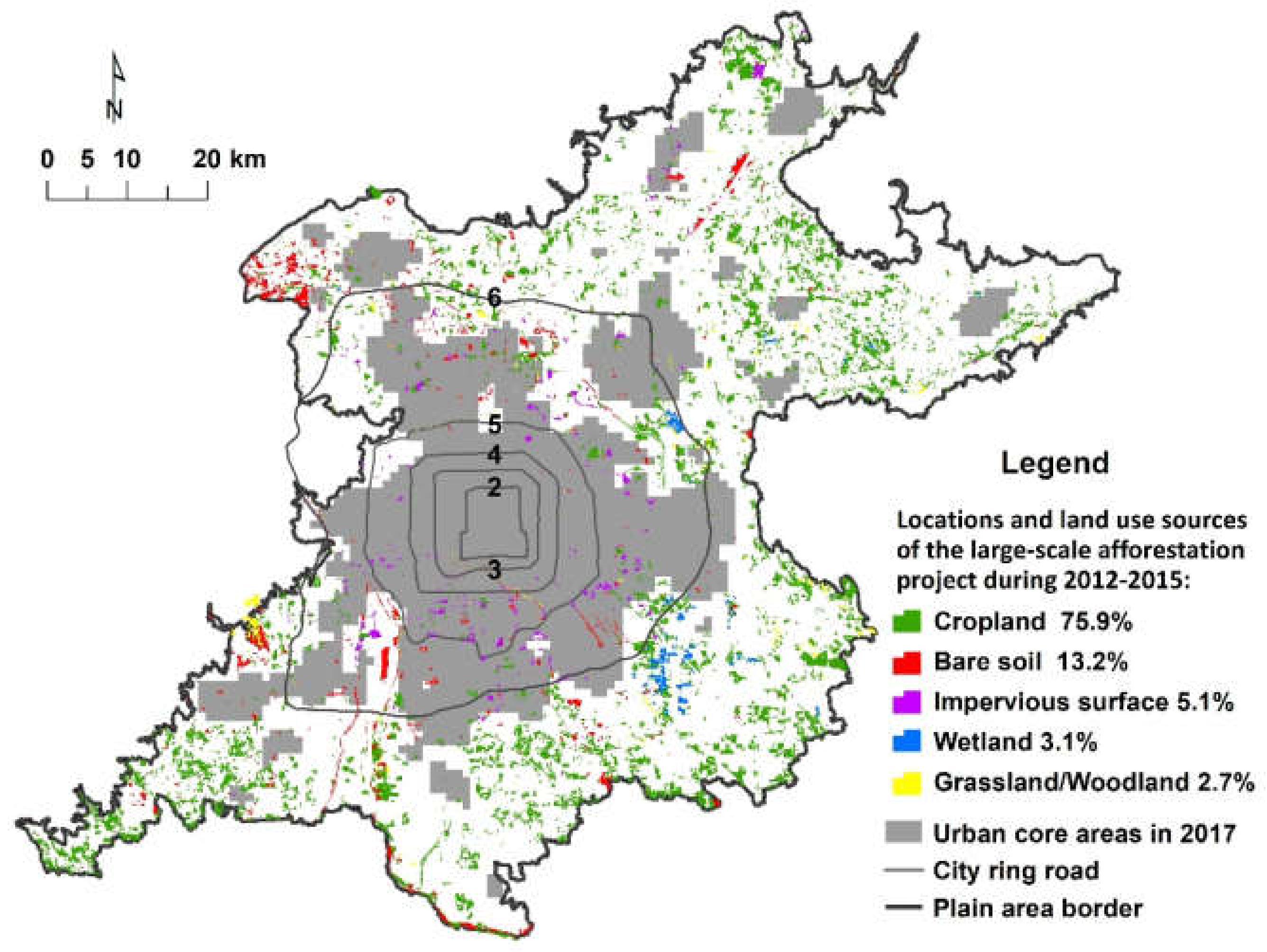
2.2.2. Identification of the Planting Sites

According to the official Eighth Census Report on Landscaping Resources of Beijing (2015), the One-Million Mu Plain Afforestation Project was the dominant greening effort in Beijing’s plain area during 2011–2015, contributing to a 10.0 increase of percent forest cover in Beijing’s plain area. Besides this, no major forest gain/loss was officially recorded during the decade of 2009–2018 under strict forestland supervision of the Bureau. As a result, other efforts that contributed to forest cover changes in the studied period were ignored.

The locations and borders of 7395 planned planting sites of the One-Million-Mu Plain Afforestation Project conducted during 2012–2015 were obtained from the Beijing Municipal Bureau of Forestry and Parks in the format of GIS shapefile. Considering deviations between planning and practice, the file was rectified based on Google Earth images captured in 2015 or 2016. Additionally, land use sources of new plantations were identified with various references, including, e.g., official documents; Google Earth images (captured in 2011); and field investigations covering 180 planting sites conducted in March, April, and November of 2013.

2.2.3. Calculation of the Diurnal and Seasonal Average LST and SUHII

MODIS LST data have been frequently used in UHI studies due to their high temporal resolution [58]. In this study, time series LST data were obtained from version 6 EOS-Aqua-MODIS LST data (MOD11A2, 8-day composite, 1 km × 1 km spatial resolution) through the Google Earth Engine [59]. We chose the Aqua satellite as it passes over Beijing at local time of 01:30 (nighttime) and 13:30 (daytime), which is closer to the lowest and highest temperature during the day compared with the Terra satellite at the local time of 22:30 (nighttime) and 10:30 (daytime). A total of 920 images covering ten years of 2009–2018 in Beijing were downloaded. Daytime/nighttime images of each year ranged from band 1 (1–8 January) to band 46 (26–31 December/25–31 December). Bands were classified and averaged according to the warm season (band 13–38, 7 April–30 October) and cold season (band 39–46 and band 1–12, 31 October–6 April) during the year, as well as the four seasons of spring (band 9–19, 6 March–1 June), summer (band 20–31, 2 June–5 September), autumn (band 32–42, 6 September–1 December), and winter (band 43–46 and band 1–8, 2 December–5 March).

A non-parametric model of the linear regression function between LST and regionalized ISA to calculate SUHII proposed by Li et al. [60] was used in this study (Figure 2). The steps applied were as follows. Firstly, a 1 km × 1 km fishnet was created within the study area considering the resolution of MODIS LST data. The proportion of water cover and ISA in each grid cell of the fishnet in the years of 2009, 2011, 2014, and 2017 was calculated. Secondly, grid cells with more than half of their total area outside the boundary and those with a water coverage higher than 0.25 were excluded. This meant that 6325 grid cells were left. Thirdly, grid cells were converted into points using the feature to point module in the Arcgis software (version 10.5; Esri, Inc., RedLands, CA, USA), and the ISA proportion was regionalized using the Kernel Density Estimation (KDE) method. The kernel radius was 3 km and the resolution of the output raster cell was 1 km. Fourth, all the output pixels within the study area were clustered based on 1% intervals of ISA_KDE. The values of ISA_KDE and LST of the same cluster were averaged to counteract the sub-interval variation of LST caused by the heterogeneity of the urban surface. Finally, the linear regression slopes of percentile-averaged ISA_KDE and LST in the years from 2009 to 2018 were calculated and defined as SUHIIs if the coefficient of determination (R²) employed to evaluate the accuracy of the function was higher than 0.8. As ISA data were not available in each year during 2009–2018, ISA_KDE in 2009 was used for the modeling in 2009 and 2010; ISA_KDE in 2011 was used for the modeling in 2011 and 2012; ISA_KDE in 2014 was used for the modeling in 2013, 2014, and 2015; and ISA_KDE in 2017 was used for the modeling in 2016, 2017, and 2018.

2.3. Statistical Analysis

2.3.1. Temporal Trend Analysis of SUHII and Pixel-Wise LST

The yearly value of SUHIIs and pixel-wise LST was averaged in three periods, i.e., Period I (2009–2011, before the planting), Period II (2012–2015, during the planting), and Period III (2016–2018, after the planting), in order to find potential rules for the changes related to the planting. Simultaneously, the temporal trends of SUHII and pixel-wise LST in time series of 2009–2018 were detected by using the Mann–Kendall (MK) [61,62] and Sen’s slope estimator [63] non-parametric tests to further detect the rules. The MK test was used to disclose the statistical significance of the trend in time series, and the Sen’s slope estimation was employed to discover the trend magnitude. These two methods have been widely used in climate and environmental research because no distributional hypotheses for the variables are required [28,64]. The calculation of the MK and Sen’s slope test was conducted using the mkttest function of the modifiedmk package, and the sqmk function of trendchange package with R (version 3.3.1; R Development Core Team, Vienna, Austria). The visualization of pixel-wise variables was realized in Arcgis 10.5.

2.3.2. Regression Analysis of LST Changes in Response to the ISA Dynamic and Afforestation

Basic data on the variables, including the LST, ISA_KDE, and new plantation areas in the 6325 grid cells (1 km*1 km) covering the study area described above in Section 2.2.3 were collected. The average LST of Period I and III in each grid and its increase from Period I to III were calculated, and recorded as ΔLST. Similarly, the increase of ISA_KDE from Period I (ISA_KDE2011) to Period III (ISA_KDE2017) in each grid was computed, and recorded as ΔISA_KDE. The area of new plantations in each grid was also regionalized using the Kernel Density Estimation (KDE) method following the same steps in Section 2.2.3 and was named FOR_KDE.

The ordinary least squares (OLS) model was used as a conventional regression model to estimate geographical issues [65]. It was adopted in this study to figure out the general effects of ISA change and large-scale afforestation on LST changes from a global view of the study area. The process of OLS estimation was realized using the Ordinary Least Squares module in Arcgis 10.5. Furthermore, in order to unveil the individual contribution of ISA change and afforestation to SUHII change, the data were divided into two sub-datasets of “ISA unchanged” and “ISA changed”, as well as “without new plantations” and “with new plantations”, following the steps displayed in the Supplementary file (Figure S1). To counteract the sub-interval variations caused by spatial heterogeneity, processes to obtain the pixel group and data average were conducted following the 1% intervals clustering method, as described in Section 2.2.3. A linear regression simulation was chosen as the preferential model and was realized using Microsoft Excel 2016. For scatter diagrams that showed evident trend transition and inflection points, a piecewise linear regression simulation was conducted to improve the model reliability using the segmented function of the segmented package with R software.

2.3.3. Scenario Prediction

As previous studies have proved that artificial surfaces and green space determine LST variations in all seasons [17,20], it was hypothesized that LST change was only caused by the combined effects of ISA change and the planting project. To unveil the share of contributions of ISA change and afforestation to SUHII variation in different time divisions, the controlled regression models mentioned in Section 2.3.2 using sub-datasets of “ISA unchanged” and “without new plantations” were employed. Regression models of higher correlation coefficients were selected to predict ΔLST from Period I to Period III under two scenarios: (A) Without the afforestation project, and (B) without ISA change during the transition from Period I to Period III. The actual SUHII of different time divisions in Period I and Period III, as well as the predicted SUHII in Period III under the two scenarios, was calculated. Finally, the actual and predicted SUHII increases from Period I to Period III were compared, and the difference could be attributed to the assumption of “without the afforestation project” or “without ISA change”. Therefore, the contribution shares were uncovered.

3. Results

3.1. ISA Dynamics, Location of the Planting Sites, and SUHII Changes

The accuracy of land cover classification of 2009, 2011, 2014, and 2017 was 87.9%, 85.3%, 88.2%, and 82.3%, respectively. The ISA percentage in the plain area of Beijing consistently increased from 38.1% in 2009 to 44.7% in 2017 (Figure 3). The ISA increment seems to be more intense near and outside the Sixth Ring Road. When urban core areas and suburb/rural areas were zoned by the contour line of ISA_KDE of 50% [28], the ratio of urban core areas increased from 1752 km² in 2009 to 2075 km² in 2017. The expansion of urban core areas seems to be more obvious in northeastward and southward directions.

The locations and land use sources of 7395 planting sites of the project are shown in Figure 4. According to the statistical results, we found that the project has accomplished the target of a 10.0 increase of percent forest cover in Beijing’s plain area. Most of the planting was arranged outside the urban core areas, as 81.7% of the planting area was distributed outside the Sixth Ring Road, 16.6% between the Sixth and Fifth Ring Road, and 1.68% inside the Fifth Ring Road. The influence of land use sources of new plantations on LST change was ignored in this study because most of the planting sites were converted from the same land cover type, i.e., cropland (75.9%).

The process of SUHII quantification during 2009–2018 following the linear regression method is displayed in the Supplementary Material (Figure S2), as are the calculation results (Tables S1 and S2). The regression functions seem well-fitted in all of the time divisions, except for spring days, winter days, and cold season days, which have R² values generally lower than 0.8. The highest SUHII across a year occurred on summer days, ranging from 6.17 to 9.26, followed by winter nights, ranging from 5.48 to 8.00, while the lowest SUHII occurred on autumn days, varying from 2.19 to 3.96.

Table 1. Results of Mann–Kendall (MK) and Sen’s slope tests of SUHIIs during the years from 2009 to 2018.

Time	Statistical Parameter	Spring	Summer	Autumn	Winter	Warm Season	Cold Season
Daytime	ZMK	-	2.33	−0.18	-	3.22	-
	QSen	-	0.22	−0.04	-	0.12	-
	p-value	-	0.02 *	0.86	-	0.00 *	-
Nighttime	ZMK	1.43	0.36	1.43	2.68	0.89	2.5
	QSen	0.13	0.04	0.1	0.21	0.03	0.18
	p-value	0.15	0.72	0.15	0.01 *	0.37	0.01 *

Z_MK is the statistical detection value of the MK test, where positive values of Z_MK indicate increasing trends and negative Z_MK values show decreasing trends; and Q_Sen is the Sen’s slope value and the absolute value of Q_Sen can be interpreted as the changing magnitude. * Statistically significant trends at the 5% significance level.

reveals the SUHII with a yearly rising tendency in all diurnal and seasonal divisions during 2009–2018, except for autumn days, because all of the values of Z_MK are positive, in addition to autumn days. SUHII for summer days, winter nights, warm season days, and cold season nights increased significantly. Sen’s slope values of SUHII for these four time divisions were higher than others, indicating higher growth rates of SUHII.

Average SUHIIs in the three periods divided by the planting project showed a consistent rise in all of the time divisions (values available), except for autumn days, summer nights, and warm season nights (Figure 5). Considering the results above, the focus in the subsequent study was on summer days, winter nights, warm season days, and cold season nights, as SUHII and its increase in these four time divisions were more evident.

3.2. Distribution of the Regionalized ISA Increment, Regionalized Planting Areas, and Changing Magnitude of Pixel-Wise LST

Figure 6a,b reveal that high values of ISA_KDE and FOR_KDE are mainly distributed near or outside the Sixth Ring Road. Sen’s slope values representing the changing magnitude of LST are similarly distributed in summer days and warm season days, i.e., high values are mainly found in the south, especially outside the Sixth Ring Road, where lots of pixels have experienced a significant LST increase; low values are generally distributed in the northwest zone, and a few pixels have experienced a significant LST decrease (Figure 6c,e). However, during winter nights and cold season nights, the distribution was different, i.e., high-value areas are mainly inside or around the Sixth Ring Road, especially in the south, where a few clustered pixels display a significant LST increase; low-value areas are generally located in the northeast and southeast, and very few pixels show a significant LST decrease (Figure 6d,f). This disparity suggests different driving mechanisms of LST changes during warm season days and cold season nights.

3.3. LST Changes in Response to ISA Dynamics and Afforestation

Distributions of the average LST in the three periods are displayed in the Supplementary Materials, Figure S2.

Table 2. Ordinary least squares (OLS) estimation results of ΔLST in relation to FOR_KDE and ΔISA_KDE.

Time	Variable	Coefficient	Std Error	t-Statistic	Probability	Observations	R2	Adjusted R2	AICs
Summer day	FORKDE	−0.0024	0.00	−2.38	0.0174 *	6325	0.1273	0.1270	13701
	ΔISAKDE	0.0408	0.00	30.18	0.0000 *
	Intercept	0.5281	0.01	37.66	0.0000 *
Winter night	FORKDE	−0.0173	0.00	−27.00	0.0000 *	6325	0.2247	0.2245	7847
	ΔISAKDE	−0.0235	0.00	−27.60	0.0000 *
	Intercept	1.2660	0.01	143.42	0.0000 *
Warm season day	FORKDE	0.0012	0.00	1.20	0.2314	6325	0.1159	0.1156	1302
	ΔISAKDE	0.0360	0.00	28.04	0.0000 *
	Intercept	−0.0908	0.01	−6.83	0.0000 *
Cold season night	FORKDE	−0.0154	0.00	−25.87	0.0000 *	6325	0.1929	0.1926	6962
	ΔISAKDE	−0.0188	0.00	−23.67	0.0000 *
	Intercept	1.1680	0.01	141.90	0.0000 *

* Statistically significant trends at the 5% significance level. AIC, the Akaike information criterion (AIC). The best model is determined with the smallest AIC value.

reveals that FOR_KDE was significantly negatively correlated with ΔLST during summer days, winter nights, and cold season nights, but insignificantly positively correlated with ΔLST on warm season days. ΔISA_KDE was significantly positively correlated with ΔLST on summer days and warm season days, and significantly negatively correlated with ΔLST during winter nights and cold season nights. On summer days, the regression coefficient between ΔISA_KDE and ΔLST was nearly 20 times the coefficient between FOR_KDE and ΔLST, indicating a substantial difference of contribution magnitudes to ΔLST. However, during winter nights and cold season nights, the regression coefficient between ΔISA_KDE and ΔLST was slightly larger than that between FOR_KDE and ΔLST, suggesting a similar magnitude of contribution to LST.

In total, 499 pixels with a zero value of FOR_KDE and 468 pixels with a zero value of ΔISA_KDE were found among all of the 6325 pixels (Figure 7a or Figure 8a). In the groups with zero-valued ΔISA_KDE, the average ΔLST showed a downward trend as FOR_KDE increased in all four time divisions, which indicates that afforestation can restrict the LST increase on both warm season days and during cold season nights (Figure 7c–f). In groups with nonzero-valued ΔISA_KDE, the average ΔLST also showed a downward trend as FOR_KDE increased on summer days and warm season days; however, during winter nights and cold season nights, there was an inflection point, after which the trend reversed. This may be caused by the difference in the positive and negative ΔISA_KDE value before and after the inflection point, reflected in Figure 7b, as the LST change in the group of nonzero-valued ΔISA_KDE was related to the combined effects of afforestation and ISA change. It was also noticed that on summer days and warm season days, the group with nonzero-valued ΔISA_KDE generally had a higher ΔLST compared with zero-valued ΔISA_KDE, while during winter nights and cold season nights, the group with nonzero-valued ΔISA_KDE had lower ΔLST. This phenomenon manifests the heating effect of impervious surfaces on warm season days and the cooling effect during cold season nights, which conforms to the above OLS estimation results.

Likewise, in groups with zero-valued FOR_KDE, the average ΔLST showed an upward trend as ΔISA_KDE increased on summer days and warm season days (Figure 8c,e), and there was a turning point (ΔISA_KDE equals 0.217), after which the slope increased. During winter nights and cold season nights, the average ΔLST firstly showed a downward trend along the gradient of ΔISA_KDE, and then exhibited a slightly upward trend when ΔISA_KDE was higher than 0.096 during winter nights and 0.034 during cold season nights (Figure 8d,f). This indicates that ISA expansion can accelerate the LST increase on warm season days, especially when ΔISA_KDE exceeds 0.217, and can restrict the LST increase during cold season nights within certain thresholds. ΔLST in the groups with nonzero-valued FOR_KDE displayed a similar trend to the groups with zero-valued FOR_KDE on summer days and warm season days. During winter nights and cold season nights, however, the trends were different. The average ΔLST firstly showed an upward trend within a ΔISA_KDE value of −9.5 and −9.6 during winter nights and cold season nights, respectively. Then, the trend reversed beyond the threshold value. It could be noticed that this trend transition was closely related to the average FOR_KDE dynamic along the ΔISA_KDE gradient revealed in Figure 8b. The values of ΔLST in the group with nonzero-valued FOR_KDE were generally lower than in the group with zero-valued FOR_KDE, from which the cooling effect of afforestation during cold season nights can be derived.

3.4. Contributions of ISA Change and Afforestation to SUHII Increases

SHUIIs of the four time divisions in Period I and III, as well as predicted scenarios of Period III, were calculated using the linear regression model (Figure 9). Models selected from Section 3.3 to predict ΔLST in the two scenarios include the piecewise regression models of ΔLST and ΔISA_KDE on summer days and warm season days in the groups with zero-valued FOR_KDE, as well as linear regression models of ΔLST and FOR_KDE during winter nights and cold season nights in the groups with zero-valued ΔISA_KDE.

As shown in Figure 9, SUHII on summer days increased by 1.40 from Period I (7.47) to III (8.87), whereas, without the planting project, the increase should have been 0.37. This indicates that the ISA change contributed 26.4% of the total SUHII increase on summer days, and the remaining 73.6% increase was caused by afforestation. Similarly, on warm season days, the ISA change contributed 17.1% of the SUHII increase, and the remaining 82.9% increase was caused by afforestation (

Table 3. Contributions of the ISA change and afforestation to SUHII increases derived from the difference of the actual and predicted SUHII in the two scenarios from Period I to Period III.

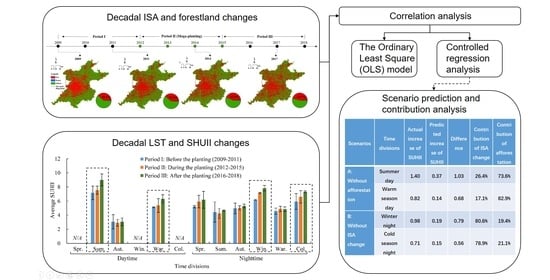
Scenarios	Time Divisions	Actual Increase of SUHII	Predicted Increase of SUHII	Difference	Contribution of ISA Change	Contribution of Afforestation
A: Without afforestation	Summer day	1.40	0.37	1.03	26.4%	73.6%
	Warm season day	0.82	0.14	0.68	17.1%	82.9%
B: Without ISA change	Winter night	0.98	0.19	0.79	80.6%	19.4%
	Cold season night	0.71	0.15	0.56	78.9%	21.1%

). SUHII during winter nights increased by 0.98 from Period I (6.40) to III (7.38), whereas, without ISA change, the increase should have been 0.19. This suggests that afforestation led to 19.4% of the SUHII increase during winter nights, and the remaining 80.6% increase was induced by ISA change. Similarly, during cold season nights, 19.4% of the SUHII increase was caused by afforestation and the remaining 78.9% was attributed to ISA change. Altogether, afforestation had the dominant effect on increasing SUHII on warm season days, while ISA change had the major effect on increasing SUHII during cold season nights.

4. Discussion

4.1. Spatial-Temporal Changes of ISA, Urban Forests, and SUHII in Beijing’s Plain Area

The study revealed that the percent of ISA in the plain area of Beijing increased by 6.6 from 2009 to 2017. Previous studies depicting the urbanization dynamics of Beijing showed divergent results because of disparities of data sources, geographic extents, urban area definitions, and time ranges, etc. [66,67,68]. A shared phenomenon was that ISA and urban areas in Beijing had a consistent increasing tendency during the past decades, and the urban–rural fringe generally extended to the northeast and south, especially near and outside the Sixth Ring Road.

The ratio of forest cover in Beijing’s plain area increased by 10.0 due to the large-scale afforestation project from 2012 to 2015. However, according to the study of Huang et al. [69], only 52.34% of the total afforested/reforested area could be recognized by Landsat remote sensors in 2015. One of the reasons for this may be that most of the new forestland was converted from cropland. These two land cover types are easily confused because of their similar reflectance. Another important reason may be that there is a growing stage in which the trees are “green” enough to be captured through remote sensing. Similarly, ecological services of the new plantations, such as environment cooling, could also have a development period, and that is why, in the present study, the ten year range was divided into three periods according to the planting stage.

The regression analysis method applied in this study to calculate SUHII avoided the problem of defining urban–rural boundaries that can cause variations in the results [41,42,70]. It is based on a strong linear relationship between LST and the percent of ISA in all the year-round seasons [60,71]. However, in this study, the correlation coefficient between LST and ISA_KDE for cold season days was relatively low, which requires further discussion. These time divisions were omitted in the next steps. Seasonal and diurnal SUHIIs were characterized by higher values on summer days and during winter nights based on this study, which is in line with previous studies [41,72]. Moreover, it was discovered that during warm season days and cold season nights, SHUII in Beijing’s plain area showed a significant rising tendency from 2009 to 2018 (also from Period I to Period III ). Meng et al. [73] similarly concluded that during 2003 and 2014 in Beijing, SUHII exhibited a fluctuating increasing trend during summer days, and the same during the nights of all seasons, except for summer. However, the study of Liu et al. [43] revealed that the SUHII of Beijing during summer days showed a fluctuating increasing trend from 2003 to 2009, but from 2010 to 2018, it showed a fluctuating decreasing trend. The bias may be caused by different geographical focuses of Beijing and the calculation methods of SUHII.

4.2. The Combined Effects of ISA Change and the Greening Project on LST and SUHII

Through OLS estimation, it was found that afforestation and ISA changes together can only explain 11.59% to 22.47% of LST changes. However, previous studies have confirmed that the proportions of impervious surface (IS) and green spaces have a dominant effect on LST spatial differentiation [17,20]. The reason for this may be that the driving mechanism of LST changes in relation to LULC conversion is more complicated than with LULC patterns because of diversified conversion types and climate effects. OLS estimation may not be a perfect model for the studied variables, as it is based on a linear-based hypothesis and there is an assumption that the error terms are independent.

The results of OLS estimation showed that ΔISA_KDE and ΔLST had a significant positive correlation on warm season days, and a significant negative correlation during cold season nights. In studies of pattern analysis, however, urban impervious surfaces and LST commonly show positive correlations during both the summer daytime/nighttime and winter nighttime [74,75]. Moreover, the results showed that FOR_KDE and ΔLST had a significant negative correlation on summer days, and the absolute value of the coefficient was much lower than that between ΔISA_KDE and ΔLST. This showed a stronger role of ISA change of the same area in influencing LST on summer days, which is in accordance with previous studies [33,34,35]. During winter nights, the role of FOR_KDE in decreasing LST was similar to that of ΔISA_KDE with the same area. This result matches the study of Duncan et al. [76], which showed that an increase in urban vegetation within a location reduces the LST in both summer and winter. However, it also challenges studies which concluded that increased greenery could reduce temperatures in summer, but increase them in winter [77,78]. The different results may be caused by the imparity of former land cover types at the revegetated sites, as well as the geographic and climatic context of studied areas.

The controlled regression analysis characterized the relationships between ΔLST, FOR_KDE, and ΔISA_KDE more precisely, as it discussed the individual effects of FOR_KDE and ΔISA_KDE on LST changes, respectively. When ΔISA_KDE equaled zero, the relationship between ΔLST and FOR_KDE was similar to the result generated from OLS estimation, i.e., FOR_KDE decreased ΔLST both on warm season days and during cold season nights. A 10% increase of FOR_KDE resulted in a decrease of 0.53 °C of LST on summer days, and a decrease of 1.11 °C of LST during winter nights. This outcome is inconsistent with a previous study which concluded that vegetation cooling is generally stronger during the daytime periods, in warm seasons, in low-latitude zones, while in the opposite context, vegetation warming usually occurs [78]. The reason for this may be that most of the new plantations from the project were transformed from cropland; the effect of this conversion on influencing LST can be counteracted by the pre-existing role of previous land cover. When FOR_KDE equaled zero, the relationship between ΔLST and ΔISA_KDE was different from the result of OLS estimation. On summer days and warm season days, a threshold of ΔISA_KDE in relation to ΔLST was found, i.e., the magnitude of IS warming could be accelerated when ΔISA_KDE exceeded 0.217 (about four times stronger than that when ΔISA_KDE was below 0.217). During winter nights and cold season nights, a turning point of ΔISA_KDE in relation to ΔLST was found (0.096 during winter nights and 0.034 during cold season nights), after which the negative correlation between ΔISA_KDE and ΔLST reversed. This phenomenon implies that the effect of the IS dynamic on LST change is not monotonous. IS expansion heats the surface on warm season days, and the warming effect can be exacerbated after IS expansion reaches certain thresholds. During cold season nights, both IS shrinkage and strong IS expansion cause surface warming. The former could generally have been caused by land use conversion, but the latter was mainly caused by anthropogenic heat releases.

Seasonal variability of the LST changing pattern and SUHII was observed in this study, as well as in previous research [72,77,79,80], suggesting different driving mechanisms between year-round time divisions. When we assumed that LST variations during 2009–2018 in the plain area of Beijing were only caused by the combined effects of ISA changes and the planting project, it was found that 82.9% of the SUHII rise on warm season days (and 73.6% on summer days) was caused by the percent forest cover increase of 10.0, and 80.6% of the SUHII increase during cold season nights (and 78.9% during winter nights) could be attributed to the percent ISA increase of 6.6. This result conforms to the previous finding that SUHII on summer days is closely related to vegetation activity and anthropogenic heat releases, while during winter nights, SUHII is strongly linked to the albedo, built-up intensity (or night-time light), and anthropogenic heat releases [72,79]. However, for the first time, a quantitative relationship was demonstrated in this study. The mechanism behind SUHII changes may be as follows: On summer days and warm season days, large-scale afforestation in the peri-urban and rural areas lowered the regional ΔLST and enlarged the gap between the LST of urban and rural areas. IS expansion formed new urban areas and had a warming effect in these regions. Therefore, afforestation and ISA changes acted synergistically to increase SUHII. During winter nights and cold season nights, peri-urban and rural afforestation still decreased the regional ΔLST, thus increasing the gap between the LST of urban and rural areas. A small amount of slight ISA shrinkage in the high-urbanized areas increased the regional ΔLST, a large amount of medium ISA expansion in the suburban areas reduced the regional ΔLST, and a small amount of extensive ISA expansion in the rural areas (e.g., construction of the new Daxing Airport in the southern city periphery) increased the regional ΔLST. As a result, the scatter points of LST and ISA_KDE in Period III showed a “U” shape trend compared with the predicted Scenario B, and the linear regression slope was eventually higher than that in the predicted scenario.

4.3. Implications for Future Landscape Planning for Urban Thermal Environment Regulation

This study characterized the combined effects of IS change and afforestation on LST and SUHII variations based on a spatial-temporal analysis of Beijing’s plain area during 2009–2018. The results can provide important insights on UHI alleviation concerning IS and green space planning in a global context of rapid urbanization [29,67,81,82] and an anticipated new development stage when abundant urban (region) greening can be conducted to help cool the city [22,83]. First, large-scale afforestation in the periphery of built-up areas in Beijing was found to have a counterproductive effect on UHI attenuation. This was caused by a singular view of vegetation cooling, rather than considering the whole area and adapting the greening to the features of the IS distribution and its development. Therefore, it is recommended that IS and green spaces should be planned jointly in coping with the UHI effect.

Second, distinct diurnal and seasonal variations of LST and SUHII changes in response to ISA and forest cover dynamics were observed. On warm season days, LST change was more sensitive to the IS dynamic compared to vegetation change of the same area, while during winter nights, the difference was much smaller. SHUII changes in response to IS and vegetation cover variations seem to be more complex as the placing of IS and vegetation cover changes also matter. For example, in this study, the contribution of a 10.0% increase of vegetation cover versus a 6.6% increase of ISA to the SUHII increase was about 3:1 on summer days, but 1:4 during winter nights. Therefore, it is suggested that city planners are season-oriented when facing the task of UHI mitigation.

Third, the existence of threshold values of ISA change in influencing LST was identified. On warm season days, a greater regional ISA increase resulted in a higher LST increase, but when the regional ISA increase reached a certain threshold, the magnitude of the LST increase was exacerbated. During cold season nights, a greater regional ISA increase corresponded to a lower LST increase within a range, whereas after a threshold, a greater regional ISA increase resulted in a higher LST increase. As a result, practitioners and planners need to pay attention to the threshold of regional ISA expansion in relation to LST changes.

4.4. Limitations and Uncertainties

While our findings enrich the existing scientific knowledge of how IS and vegetation cover changes can influence the urban thermal environment, several study limitations should be highlighted. First, extra vegetation cover changes besides the afforestation project and the influence of other land cover conversions except for ISA and forest cover were omitted due to the restriction of appropriate data with a high accuracy. However, the error caused by this shortcoming is not believed to have had a major impact on the conclusions as no major forest gain/loss except for the planting project was recorded. The influence of additional land cover conversions was trivial, e.g., strict cropland protection was implemented by the government unless there was an official decision; bare soil and grassland only account for 9.7% and 1.1% of the study area, respectively; and the area of water cover was excluded during the calculation. Moreover, an in-depth analysis of urban thermal changes in response to various types of ISA and vegetated areas, and the mechanism of energy balance (natural or anthropogenic) behind this will be addressed in our future studies.

Second, inter-annual variations of meteorological elements (e.g., temperature, precipitation, and radiation level) in the same place may have influenced the results. However, those changes should be slight within a decade and given the city-wide scope. Additionally, the processes of the pixel group and data average during the calculation can reduce the spatial heterogeneity caused by this aspect. We found that the average surface LST in the whole city had a rising tendency during 2009–2018, probably partly caused by global climate change. Therefore, further studies can be conducted on the relationship between climate change and SUHII variation, but a longer time-series is needed.

Third, the revegetated areas in this study are still at an early growing stage, while the future effect of forest cover changes on LST may not be able to be interpreted in the same way. Therefore, results of longer observation periods and continuous research are needed. Moreover, the study only focused on the case of Beijing, whereas some of its conclusions may not be directly applicable elsewhere. Therefore, further work is needed in terms of global observations on the effect of LULC conversion (especially IS and vegetation cover variations) on LST and SUHII changes, in order to fully understand the characteristics of this relationship in different background climate and geographical contexts.

5. Conclusions

Knowledge of infrastructure-based interventions (especially ISA and green space regulations) to mitigate the UHI effect is imperative for planners and practitioners [7]. This study explored LST and SUHII changes in response to ISA and forest cover variations based on remote sensing analysis for the case of Beijing. The findings show that the percent of ISA and forest cover increased by 6.6 and 10.0, respectively, in the study area. SUHIIs showed significant rising tendencies during 2009–2018 in the four time divisions of warm season days, summer days, cold season nights, and winter nights. LST changes on warm season days and summer days responded positively to a regionalized ISA increase and negatively to a regionalized forest cover increase. However, during cold season nights and winter nights, LST changes responded negatively to a slight regional ISA increase, but positively to an extensive regional ISA increase, and LST variations responded negatively to a regional forest cover increase. The effect of vegetation cooling was weaker than ISA warming on warm season days, but the effect of vegetation cooling was similar to that of ISA during cold season nights. The afforestation project dominated the contribution of SUHII rise on warm season days, while ISA changes led the contribution of SUHII increase during cold season nights. Based on our results, we suggest that IS and green spaces should be planned jointly in coping with the UHI effect, strategies of UHI mitigation should be season-oriented, and the development threshold of ISA in influencing LST should be determined.

References

- Oke, T.R. The energetic basis of the urban heat island. Q. J. R. Meteorol. Soc. 1982, 108, 1–24. [Google Scholar] [CrossRef]
- Graham, D.A.; Vanos, J.K.; Kenny, N.A.; Brown, R.D. The relationship between neighbourhood tree canopy cover and heat-related ambulance calls during extreme heat events in Toronto, Canada. Urban For. Urban Green. 2016, 20, 180–186. [Google Scholar] [CrossRef]
- Ward, K.; Lauf, S.; Kleinschmit, B.; Endlicher, W. Heat waves and urban heat islands in Europe: A review of relevant drivers. Sci. Total Environ. 2016, 569–570, 527–539. [Google Scholar] [CrossRef] [PubMed]
- Li, X.; Zhou, Y.; Yu, S.; Jia, G.; Li, H.; Li, W. Urban heat island impacts on building energy consumption: A review of approaches and findings. Energy 2019, 174, 407–419. [Google Scholar] [CrossRef]
- Li, H.; Meier, F.; Lee, X.; Chakraborty, T.; Liu, J.; Schaap, M.; Sodoudi, S. Interaction between urban heat island and urban pollution island during summer in Berlin. Sci. Total Environ. 2018, 636, 818–828. [Google Scholar] [CrossRef] [PubMed]
- Wong, L.P.; Alias, H.; Aghamohammadi, N.; Aghazadeh, S.; Nik Sulaiman, N.M. Urban heat island experience, control measures and health impact: A survey among working community in the city of Kuala Lumpur. Sustain. Cities Soc. 2017, 35, 660–668. [Google Scholar] [CrossRef]
- Leal Filho, W.; Echevarria Icaza, L.; Neht, A.; Klavins, M.; Morgan, E.A. Coping with the impacts of urban heat islands. A literature based study on understanding urban heat vulnerability and the need for resilience in cities in a global climate change context. J. Clean. Prod. 2018, 171, 1140–1149. [Google Scholar] [CrossRef]
- Voogt, J.A.; Oke, T.R. Thermal remote sensing of urban climates. Remote Sens. Environ. 2003, 86, 370–384. [Google Scholar] [CrossRef]
- Kuang, W.; Liu, Y.; Dou, Y.; Chi, W.; Chen, G.; Gao, C.; Yang, T.; Liu, J.; Zhang, R. What are hot and what are not in an urban landscape: Quantifying and explaining the land surface temperature pattern in Beijing, China. Landsc. Ecol. 2015, 30, 357–373. [Google Scholar] [CrossRef]
- Kuang, W.; Yang, T.; Liu, A.; Zhang, C.; Lu, D.; Chi, W. An EcoCity model for regulating urban land cover structure and thermal environment: Taking Beijing as an example. Sci. China Earth Sci. 2017, 60, 1098–1109. [Google Scholar] [CrossRef]
- Dai, Z.; Guldmann, J.; Hu, Y. Thermal impacts of greenery, water, and impervious structures in Beijing’s Olympic area: A spatial regression approach. Ecol. Indic. 2019, 97, 77–88. [Google Scholar] [CrossRef]
- Sun, R.; Chen, L. How can urban water bodies be designed for climate adaptation? Landsc. Urban Plan. 2012, 105, 27–33. [Google Scholar] [CrossRef]
- Wang, C.; Li, Y.; Myint, S.W.; Zhao, Q.; Wentz, E.A. Impacts of spatial clustering of urban land cover on land surface temperature across Köppen climate zones in the contiguous United States. Landsc. Urban Plan. 2019, 192, 103668. [Google Scholar] [CrossRef]
- Sun, R.; Xie, W.; Chen, L. A landscape connectivity model to quantify contributions of heat sources and sinks in urban regions. Landsc. Urban Plan. 2018, 178, 43–50. [Google Scholar] [CrossRef]
- Zhou, W.; Huang, G.; Cadenasso, M.L. Does spatial configuration matter? Understanding the effects of land cover pattern on land surface temperature in urban landscapes. Landsc. Urban Plan. 2011, 102, 54–63. [Google Scholar] [CrossRef]
- Peng, J.; Xie, P.; Liu, Y.; Ma, J. Urban thermal environment dynamics and associated landscape pattern factors: A case study in the Beijing metropolitan region. Remote Sens. Environ. 2016, 173, 145–155. [Google Scholar] [CrossRef]
- Peng, J.; Jia, J.; Liu, Y.; Li, H.; Wu, J. Seasonal contrast of the dominant factors for spatial distribution of land surface temperature in urban areas. Remote Sens. Environ. 2018, 215, 255–267. [Google Scholar] [CrossRef]
- Chen, A.; Yao, L.; Sun, R.; Chen, L. How many metrics are required to identify the effects of the landscape pattern on land surface temperature? Ecol. Indic. 2014, 45, 424–433. [Google Scholar] [CrossRef]
- Chen, Y.; Yu, S. Impacts of urban landscape patterns on urban thermal variations in Guangzhou, China. Int. J. Appl. Earth Obs. 2017, 54, 65–71. [Google Scholar] [CrossRef]
- Hu, D.; Meng, Q.; Zhang, L.; Zhang, Y. Spatial quantitative analysis of the potential driving factors of land surface temperature in different “Centers” of polycentric cities: A case study in Tianjin, China. Sci. Total Environ. 2020, 706, 135244. [Google Scholar] [CrossRef]
- Yao, L.; Li, T.; Xu, M.; Xu, Y. How the landscape features of urban green space impact seasonal land surface temperatures at a city-block-scale: An urban heat island study in Beijing, China. Urban For. Urban Green. 2020, 52, 126704. [Google Scholar] [CrossRef]
- Yu, Z.; Yao, Y.; Yang, G.; Wang, X.; Vejre, H. Strong contribution of rapid urbanization and urban agglomeration development to regional thermal environment dynamics and evolution. For. Ecol. Manag. 2019, 446, 214–225. [Google Scholar] [CrossRef]
- Akinyemi, F.O.; Ikanyeng, M.; Muro, J. Land cover change effects on land surface temperature trends in an African urbanizing dryland region. City Environ. Interact. 2019, 4, 100029. [Google Scholar] [CrossRef]
- Muro, J.; Strauch, A.; Heinemann, S.; Steinbach, S.; Thonfeld, F.; Waske, B.; Diekkrüger, B. Land surface temperature trends as indicator of land use changes in wetlands. Int. J. Appl. Earth Obs. 2018, 70, 62–71. [Google Scholar] [CrossRef]
- Qiao, Z.; Tian, G.; Xiao, L. Diurnal and seasonal impacts of urbanization on the urban thermal environment: A case study of Beijing using MODIS data. ISPRS J. Photogramm. 2013, 85, 93–101. [Google Scholar] [CrossRef]
- Tran, D.X.; Pla, F.; Latorre-Carmona, P.; Myint, S.W.; Caetano, M.; Kieu, H.V. Characterizing the relationship between land use land cover change and land surface temperature. ISPRS J. Photogramm. 2017, 124, 119–132. [Google Scholar] [CrossRef]
- Nurwanda, A.; Honjo, T. The prediction of city expansion and land surface temperature in Bogor City, Indonesia. Sustain. Cities Soc. 2020, 52, 101772. [Google Scholar] [CrossRef]
- Yang, Q.; Huang, X.; Tang, Q. The footprint of urban heat island effect in 302 Chinese cities: Temporal trends and associated factors. Sci. Total Environ. 2019, 655, 652–662. [Google Scholar] [CrossRef]
- Huang, K.; Li, X.; Liu, X.; Seto, K.C. Projecting global urban land expansion and heat island intensification through 2050. Environ. Res. Lett. 2019, 14, 114037. [Google Scholar] [CrossRef]
- Tran, Y.L.; Siry, J.P.; Bowker, J.M.; Poudyal, N.C. Atlanta households’ willingness to increase urban forests to mitigate climate change. Urban For. Urban Green. 2017, 22, 84–92. [Google Scholar] [CrossRef]
- Sanchez, L.; Reames, T.G. Cooling Detroit: A socio-spatial analysis of equity in green roofs as an urban heat island mitigation strategy. Urban For. Urban Green. 2019, 44, 126331. [Google Scholar] [CrossRef]
- Nastran, M.; Kobal, M.; Eler, K. Urban heat islands in relation to green land use in European cities. Urban For. Urban Green. 2019, 37, 33–41. [Google Scholar] [CrossRef]
- Myint, S.W.; Brazel, A.; Okin, G.; Buyantuyev, A. Combined Effects of Impervious Surface and Vegetation Cover on Air Temperature Variations in a Rapidly Expanding Desert City. GISci. Remote Sens. 2013, 47, 301–320. [Google Scholar] [CrossRef]
- Jamei, Y.; Rajagopalan, P.; Sun, Q.C. Spatial structure of surface urban heat island and its relationship with vegetation and built-up areas in Melbourne, Australia. Sci. Total Environ. 2019, 659, 1335–1351. [Google Scholar] [CrossRef] [PubMed]
- Xu, H.; Lin, D.; Tang, F. The impact of impervious surface development on land surface temperature in a subtropical city: Xiamen, China. Int. J. Climatol. 2013, 33, 1873–1883. [Google Scholar] [CrossRef]
- Sun, R.; Chen, L. Effects of green space dynamics on urban heat islands: Mitigation and diversification. Ecosyst. Serv. 2017, 23, 38–46. [Google Scholar] [CrossRef]
- Shen, W.; Li, M.; Huang, C.; He, T.; Tao, X.; Wei, A. Local land surface temperature change induced by afforestation based on satellite observations in Guangdong plantation forests in China. Agric. For. Meteorol. 2019, 276–277, 107641. [Google Scholar] [CrossRef]
- Bowler, D.E.; Buyung-Ali, L.; Knight, T.M.; Pullin, A.S. Urban greening to cool towns and cities: A systematic review of the empirical evidence. Landsc. Urban Plan. 2010, 97, 147–155. [Google Scholar] [CrossRef]
- Zhou, D.; Xiao, J.; Bonafoni, S.; Berger, C.; Deilami, K.; Zhou, Y.; Frolking, S.; Yao, R.; Qiao, Z.; Sobrino, J. Satellite Remote Sensing of Surface Urban Heat Islands: Progress, Challenges, and Perspectives. Remote Sens. 2019, 11, 48. [Google Scholar] [CrossRef]
- Schwarz, N.; Lautenbach, S.; Seppelt, R. Exploring indicators for quantifying surface urban heat islands of European cities with MODIS land surface temperatures. Remote Sens. Environ. 2011, 115, 3175–3186. [Google Scholar] [CrossRef]
- Zhou, D.; Zhang, L.; Hao, L.; Sun, G.; Liu, Y.; Zhu, C. Spatiotemporal trends of urban heat island effect along the urban development intensity gradient in China. Sci. Total Environ. 2016, 544, 617–626. [Google Scholar] [CrossRef] [PubMed]
- Li, K.; Chen, Y.; Wang, M.; Gong, A. Spatial-temporal variations of surface urban heat island intensity induced by different definitions of rural extents in China. Sci. Total Environ. 2019, 669, 229–247. [Google Scholar] [CrossRef] [PubMed]
- Liu, X.; Zhou, Y.; Yue, W.; Li, X.; Liu, Y.; Lu, D. Spatiotemporal patterns of summer urban heat island in Beijing, China using an improved land surface temperature. J. Clean. Prod. 2020, 257, 120529. [Google Scholar] [CrossRef]
- Li, X.; Zhou, Y.; Asrar, G.R.; Imhoff, M.; Li, X. The surface urban heat island response to urban expansion: A panel analysis for the conterminous United States. Sci. Total Environ. 2017, 605–606, 426–435. [Google Scholar] [CrossRef] [PubMed]
- Yao, R.; Wang, L.; Huang, X.; Gong, W.; Xia, X. Greening in Rural Areas Increases the Surface Urban Heat Island Intensity. Geophys. Res. Lett. 2019, 46, 2204–2212. [Google Scholar] [CrossRef]
- Wang, W.; Shu, J. Urban Renewal Can Mitigate Urban Heat Islands. Geophys. Res. Lett. 2020, 47, e2019GL085948. [Google Scholar] [CrossRef]
- Dou, Y.; Kuang, W. A comparative analysis of urban impervious surface and green space and their dynamics among 318 different size cities in China in the past 25 years. Sci. Total Environ. 2020, 706, 135828. [Google Scholar] [CrossRef]
- Yao, N.; Konijnendijk Van Den Bosch, C.C.; Yang, J.; Devisscher, T.; Wirtz, Z.; Jia, L.; Duan, J.; Ma, L. Beijing’s 50 million new urban trees: Strategic governance for large-scale urban afforestation. Urban For. Urban Green. 2019, 44, 126392. [Google Scholar] [CrossRef]
- Wu, W.; Zhao, S.; Zhu, C.; Jiang, J. A comparative study of urban expansion in Beijing, Tianjin and Shijiazhuang over the past three decades. Landsc. Urban Plan. 2015, 134, 93–106. [Google Scholar] [CrossRef]
- Li, X.; Zhou, W.; Ouyang, Z. Forty years of urban expansion in Beijing: What is the relative importance of physical, socioeconomic, and neighborhood factors? Appl. Geogr. 2013, 38, 1–10. [Google Scholar] [CrossRef]
- Guo, M.; Chen, S.; Wang, W.; Liang, H.; Hao, G.; Liu, K. Spatiotemporal variation of heat fluxes in Beijing with land use change from 1997 to 2017. Phys. Chem. Earth Parts A/B/C 2019, 110, 51–60. [Google Scholar] [CrossRef]
- Liu, K.; Su, H.; Li, X.; Wang, W.; Yang, L.; Liang, H. Quantifying spatial--temporal pattern of urban heat island in Beijing: An improved assessment using land surface temperature (LST) time series observations from LANDSAT, MODIS, and Chinese new satellite GaoFen-1. IEEE J. Sel. Top. Appl. Earth Obs. Remote Sens. 2016, 9, 2028–2042. [Google Scholar] [CrossRef]
- Song, X.; Wang, S.; Li, T.; Tian, J.; Ding, G.; Wang, J.; Wang, J.; Shang, K. The impact of heat waves and cold spells on respiratory emergency department visits in Beijing, China. Sci. Total Environ. 2018, 615, 1499–1505. [Google Scholar] [CrossRef] [PubMed]
- Xu, H. Modification of normalised difference water index (NDWI) to enhance open water features in remotely sensed imagery. Int. J. Remote Sens. 2007, 27, 3025–3033. [Google Scholar] [CrossRef]
- Deng, C.; Wu, C. BCI: A biophysical composition index for remote sensing of urban environments. Remote Sens. Environ. 2012, 127, 247–259. [Google Scholar] [CrossRef]
- Ridd, M.K. Exploring a VIS (vegetation-impervious surface-soil) model for urban ecosystem analysis through remote sensing: Comparative anatomy for cities. Int. J. Remote Sens. 1995, 16, 2165–2185. [Google Scholar] [CrossRef]
- Baig, M.H.A.; Zhang, L.; Shuai, T.; Tong, Q. Derivation of a tasselled cap transformation based on Landsat 8 at-satellite reflectance. Remote Sens. Lett. 2014, 5, 423–431. [Google Scholar] [CrossRef]
- Wan, Z. New refinements and validation of the MODIS Land-Surface Temperature/Emissivity products. Remote Sens. Environ. 2008, 112, 59–74. [Google Scholar] [CrossRef]
- Gorelick, N.; Hancher, M.; Dixon, M.; Ilyushchenko, S.; Thau, D.; Moore, R. Google Earth Engine: Planetary-scale geospatial analysis for everyone. Remote Sens. Environ. 2017, 202, 18–27. [Google Scholar] [CrossRef]
- Li, H.; Zhou, Y.; Li, X.; Meng, L.; Wang, X.; Wu, S.; Sodoudi, S. A new method to quantify surface urban heat island intensity. Sci. Total Environ. 2018, 624, 262–272. [Google Scholar] [CrossRef]
- Mann, H.B. Nonparametric tests against trend. Econom. J. Econom. Soc. 1945, 13, 245–259. [Google Scholar] [CrossRef]
- Kendall, M.G. Rank Correlation Methods; Griffin: London, UK, 1975. [Google Scholar]
- Sen, P.K. Estimates of the regression coefficient based on Kendall’s tau. J. Am. Stat. Assoc. 1968, 63, 1379–1389. [Google Scholar] [CrossRef]
- Chen, J.; Lyu, Y.; Zhao, Z.; Liu, H.; Zhao, H.; Li, Z. Using the multidimensional synthesis methods with non-parameter test, multiple time scales analysis to assess water quality trend and its characteristics over the past 25 years in the Fuxian Lake, China. Sci. Total Environ. 2019, 655, 242–254. [Google Scholar] [CrossRef] [PubMed]
- Butler, N.A. The efficiency of ordinary least squares in designed experiments subject to spatial or temporal variation. Stat. Probabil. Lett. 1999, 41, 73–81. [Google Scholar] [CrossRef]
- Peng, J.; Hu, Y.; Liu, Y.; Ma, J.; Zhao, S. A new approach for urban-rural fringe identification: Integrating impervious surface area and spatial continuous wavelet transform. Landsc. Urban Plan. 2018, 175, 72–79. [Google Scholar] [CrossRef]
- Chen, W.; Zhang, Y.; Pengwang, C.; Gao, W. Evaluation of Urbanization Dynamics and its Impacts on Surface Heat Islands: A Case Study of Beijing, China. Remote Sens. 2017, 9, 453. [Google Scholar]
- Yang, Y.; Liu, Y.; Li, Y.; Du, G. Quantifying spatio-temporal patterns of urban expansion in Beijing during 1985–2013 with rural-urban development transformation. Land Use Policy 2018, 74, 220–230. [Google Scholar] [CrossRef]
- Huang, H.; Chen, Y.; Clinton, N.; Wang, J.; Wang, X.; Liu, C.; Gong, P.; Yang, J.; Bai, Y.; Zheng, Y.; et al. Mapping major land cover dynamics in Beijing using all Landsat images in Google Earth Engine. Remote Sens. Environ. 2017, 202, 166–176. [Google Scholar] [CrossRef]
- Yao, R.; Wang, L.; Huang, X.; Niu, Y.; Chen, Y.; Niu, Z. The influence of different data and method on estimating the surface urban heat island intensity. Ecol. Indic. 2018, 89, 45–55. [Google Scholar] [CrossRef]
- Yuan, F.; Bauer, M.E. Comparison of impervious surface area and normalized difference vegetation index as indicators of surface urban heat island effects in Landsat imagery. Remote Sens. Environ. 2007, 106, 375–386. [Google Scholar] [CrossRef]
- Zhou, D.; Zhao, S.; Liu, S.; Zhang, L.; Zhu, C. Surface urban heat island in China’s 32 major cities: Spatial patterns and drivers. Remote Sens. Environ. 2014, 152, 51–61. [Google Scholar] [CrossRef]
- Meng, Q.; Zhang, L.; Sun, Z.; Meng, F.; Wang, L.; Sun, Y. Characterizing spatial and temporal trends of surface urban heat island effect in an urban main built-up area: A 12-year case study in Beijing, China. Remote Sens. Environ. 2018, 204, 826–837. [Google Scholar] [CrossRef]
- Ma, Q.; Wu, J.; He, C. A hierarchical analysis of the relationship between urban impervious surfaces and land surface temperatures: Spatial scale dependence, temporal variations, and bioclimatic modulation. Landsc. Ecol. 2016, 31, 1139–1153. [Google Scholar] [CrossRef]
- Mathew, A.; Khandelwal, S.; Kaul, N. Investigating spatial and seasonal variations of urban heat island effect over Jaipur city and its relationship with vegetation, urbanization and elevation parameters. Sustain. Cities Soc. 2017, 35, 157–177. [Google Scholar] [CrossRef]
- Duncan, J.M.A.; Boruff, B.; Saunders, A.; Sun, Q.; Hurley, J.; Amati, M. Turning down the heat: An enhanced understanding of the relationship between urban vegetation and surface temperature at the city scale. Sci. Total Environ. 2019, 656, 118–128. [Google Scholar] [CrossRef] [PubMed]
- Chun, B.; Guldmann, J. Impact of greening on the urban heat island: Seasonal variations and mitigation strategies. Comput. Environ. Urban Syst. 2018, 71, 165–176. [Google Scholar] [CrossRef]
- Su, Y.; Liu, L.; Liao, J.; Wu, J.; Ciais, P.; Liao, J.; He, X.; Liu, X.; Chen, X.; Yuan, W.; et al. Phenology acts as a primary control of urban vegetation cooling and warming: A synthetic analysis of global site observations. Agric. For. Meteorol. 2020, 280, 107765. [Google Scholar] [CrossRef]
- Peng, S.; Piao, S.; Ciais, P.; Friedlingstein, P.; Ottle, C.; Bréon, F.; Nan, H.; Zhou, L.; Myneni, R.B. Surface Urban Heat Island Across 419 Global Big Cities. Environ. Sci. Technol. 2011, 46, 696–703. [Google Scholar] [CrossRef]
- Oleson, K.W.; Bonan, G.B.; Feddema, J.; Jackson, T. An examination of urban heat island characteristics in a global climate model. Int. J. Climatol. 2011, 31, 1848–1865. [Google Scholar] [CrossRef]
- Waseem, S.; Khayyam, U. Loss of vegetative cover and increased land surface temperature: A case study of Islamabad, Pakistan. J. Clean. Prod. 2019, 234, 972–983. [Google Scholar] [CrossRef]
- Alkama, R.; Cescatti, A. Biophysical climate impacts of recent changes in global forest cover. Science 2016, 351, 600–604. [Google Scholar] [CrossRef] [PubMed]
- Dinda, S. Environmental Kuznets Curve Hypothesis: A Survey. Ecol. Econ. 2004, 49, 431–455. [Google Scholar] [CrossRef]