Weakly Supervised Change Detection Based on Edge Mapping and SDAE Network in High-Resolution Remote Sensing Images

Abstract

Change detection for high-resolution remote sensing images is more and more widespread in the application of monitoring the Earth’s surface. However, on the one hand, the ground truth could facilitate the distinction between changed and unchanged areas, but it is hard to acquire them. On the other hand, due to the complexity of remote sensing images, it is difficult to extract features of difference, let alone the construction of the classification model that performs change detection based on the features of difference in each pixel pair. Aiming at these challenges, this paper proposes a weakly supervised change detection method based on edge mapping and Stacked Denoising Auto-Encoders (SDAE) network called EM-SDAE. We analyze the difference in edge maps of bi-temporal remote sensing images to acquire part of the ground truth at a relatively low cost. Moreover, we design a neural network based on SDAE with a deep structure, which extracts the features of difference so as to efficiently classify changed and unchanged regions after being trained with the ground truth. In our experiments, three real sets of high-resolution remote sensing images are employed to validate the high efficiency of our proposed method. The results show that accuracy can even reach up to 91.18% with our method. In particular, compared with the state-of-the-art work (e.g., IR-MAD, PCA-k-means, CaffeNet, USFA, and DSFA), it improves the Kappa coefficient by 27.19% on average.

1. Introduction

1.1. Background and Motivation

With the technological development of various satellite remote sensors, the past decade has witnessed the increasing number of emergences of new applications based on high resolution remote sensing images, including land cover transformation [1,2,3], natural disaster evaluation [4,5,6], etc., For example, when an earthquake occurred, in order to implement timely and effectively emergency rescue and repairing work, we must efficiently evaluate the affected area and further understand the scope of the earthquake hazard. Such applications have a common requirement—identifying the changed regions on Earth’s surface as quickly and accurately as possible. To this end, we need to analyze a series of remote sensing images that are acquired over the same geographical area at different times, and further detect the changes between them. It is well established that, in order to better represent spatial structure and texture characteristics, high-resolution remote sensing images possess a high spatial resolution, in which each pixel only contains less information. This makes existing research for medium- and low-resolution images difficult to extract information from high-resolution remote sensing images and detect their changes efficiently [7,8]. Therefore, it is necessary to propose an efficient change detection method for high-resolution remote sensing images.

Change detection for remote sensing images aims to divide image pairs into changed or unchanged regions, the essence of which is a classification problem. On this basis, its main goals are to construct the feasible classification model that reflects the relationship between pixel pairs and attributes (changed or unchanged), and then find the optimal solution of the model [9]. Reckoned with the complexity of information richness and massive noises in the high-resolution images, there are two challenges for implementing change detection.

Challenge 1: difficult to intelligently acquire the high-quality ground truth. The ground truth reflects the changes in the real world, which plays a key role in the seeking of the optimal solution of the classification model. Unfortunately, the high-quality ground truth is hard to acquire because it not only requires a number of technical staff to provide a rich experience and professional judgment but also requires a large amount of time to analyze the changes of image pair [10]. In this case, as for our concerned emergency scenarios with diverse and rapid changes (e.g., natural disaster evaluation and land cover transformation), those time-consuming methods that depend on large-scale ground truth would be not practical [11,12]. Recently, the unsupervised change detection methods that directly utilize linear transformation theory to mine the ground truth are proposed, which can substitute manual tagging work and further solve the above issues to a certain extent [13,14,15]. However, the lower quality ground truth affects their detection accuracy [16,17]. Thus, how to intelligently acquire as high-quality ground truth as possible is our first technical challenge.

Challenge 2: difficult to extract features of difference. The imaging would be affected by weather, light, radiation, and even different satellites, which causes the difference characteristics of the image pair to be ambiguous [18]. Therefore, it is difficult to extract the features of difference in the remote sensing images, let alone the construction of the classification model that reflects the relationship between features of difference in the pixel pair and attributes. The existing literature utilized various classification models to divide remote sensing image pair into changed and unchanged regions, in which deep learning model is one of the most promising solutions [19,20,21,22]. Compared with other models (e.g., machine learning [23,24]), deep learning methods have advantages in dealing with data with enormous quantity and complex features. However, in the face of the remote sensing images with multiple change types and lots of noises, the detection accuracy of these methods would get lower [25,26]. Thus, how to design a more efficient classification model for extracting features of difference becomes our second technical challenge.

1.2. Proposed Method

In this paper, we propose a weakly supervised change detection framework based on edge mapping and Stacked Denoising Auto-Encoders (SDAE), which contains two detection stages: pre-classification and classification. Firstly, we design a pre-classification algorithm, which analyzes the difference of the edge maps of image pair to acquire the obviously changed or unchanged region. Moreover, the algorithm could efficiently decrease the effect of image noise and further provide the relatively reliable label data for the classification stage, because it mainly focuses on the image regions around the edges instead of the whole images. Secondly, we design a classification model based on SDAE with a deep structure to achieve the superior fitting ability. In particular, we utilize the remote sensing images that have been injected with Gaussian noise to train SDAE so as to make it possess the de-noise capability.

1.3. Key Contributions

The contributions of this paper are regarded as the following to be four-fold.

• Aiming at high-resolution remote sensing images, a novel weakly supervised change detection framework based on edge mapping and SDAE is proposed, which can extract both the obvious and subtle change information efficiently.
• A pre-classification algorithm based on the difference of the edge maps of the image pair is designed to obtain prior knowledge. Besides, a selection rule is defined and employed to select as high-quality label data as possible for the latter classification stage.
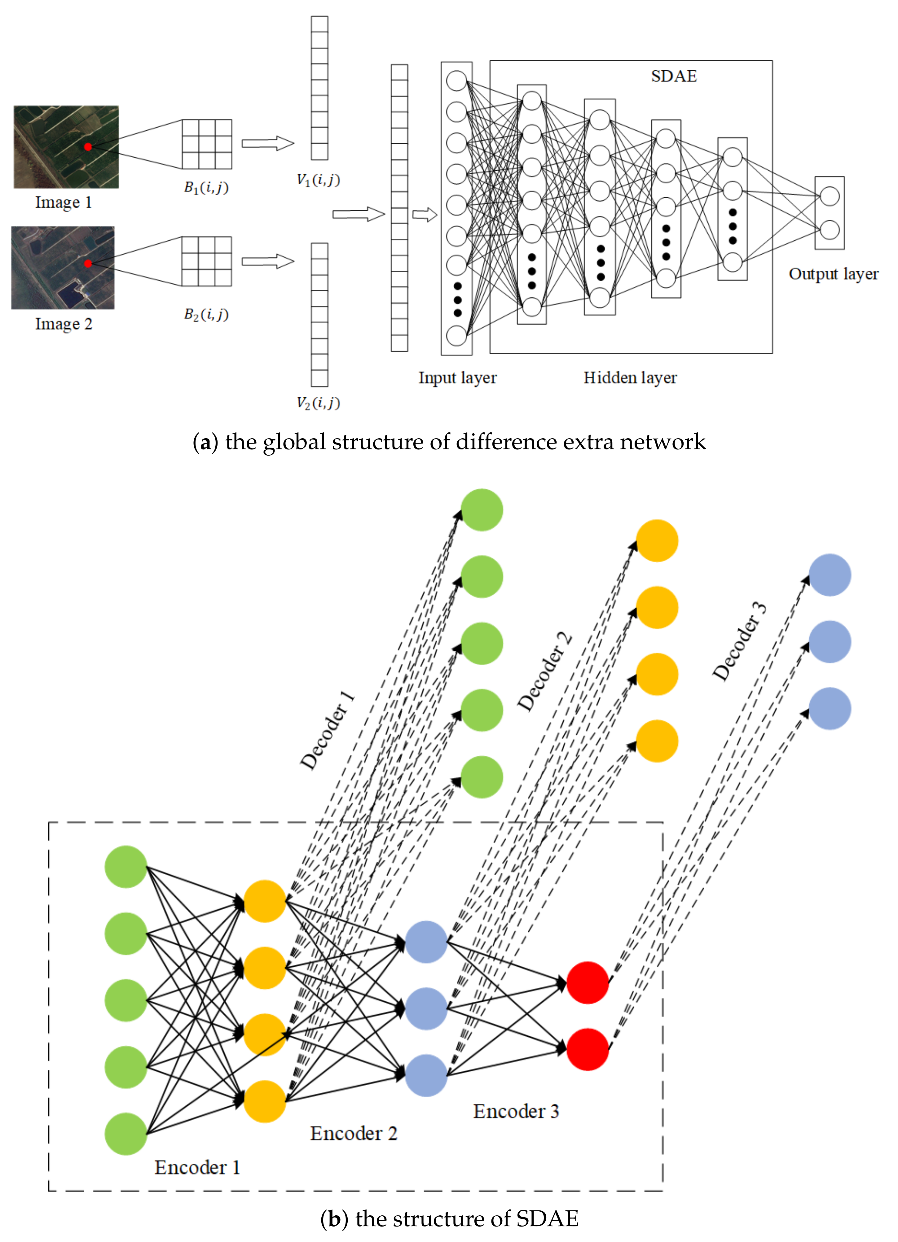
• SDAE-based deep neural networks are designed to establish a classification model with strong robustness and generalization capability, which reduces noises and extracts the features of difference of image pair. The classification model facilitates the identification of complex regions with subtle changes and improves the accuracy of the final change detection result.
• The experimental results of three datasets prove the high efficiency of our method, in which accuracy and Kappa coefficient increase to 91.18% and by 27.19% on average in the first two datasets compared with the IR-MAD, PCA-k-means, CaffeNet, USFA, and DSFA methods [15,25,26,27,28] (The code implementation of the proposed method has been published on the website https://github.com/ChenAnRn/EM-DL-Remote-sensing-images-change-detection).

The rest of this paper is organized as follows. In Section 2, we introduce the related work. Section 3 formulates the change detection problem and Section 4 describes our proposed method, including its framework and design details. In Section 5, we carry out extensive experiments to evaluate our proposed method. Section 6 concludes this paper.

2. Related Work

With the improvement of remote sensing technology, imaging sensors could obtain many types of remote sensing data. According to the data types, change detection methods can be mainly divided into three categories: high-resolution based, synthetic aperture radar (SAR)-based, multi-spectral, or hyperspectral based [29]. Due to the rich texture information of the ground features in high-resolution remote sensing images, the applications of this type of images are more and more widespread [30,31]. Change detection for high-resolution remote sensing images, which is used to mine the knowledge of the dynamics of either natural resources or man-made structures, has become a research trend [32,33,34,35]. For example, Volpi et al. studied an efficient supervised method based on support vector machine classifier for detecting changes in high-resolution images [11]; Peng et al. proposed an end-to-end change detection method based on neural network (Unet++) for semantic segmentation, in which the labeled datasets are used to train the network [36]; Mai et al. proposed a semi-supervised fuzzy logic algorithm based on Fuzzy C-Means (FCM) to detect the change of land cover [12]; Hou et al. proposed a combination of the pixel-based and object-based method to detect the building change [37], in which the saliency and morphological construction index are extracted on the difference images, and object-based semi-supervised classification is implemented on the training set by applying random forest. However, most of these existing solutions can achieve the satisfying detection result only if large amounts of ground truth is given and the remote sensing images detected have the same or similar features of difference. Apparently, they are not applicable to our concerned land cover transformation and natural disaster evaluation, which requires a rapid and accurate detection method.

To quickly and accurately detect changes in remote sensing images under various scenes, a handful of unsupervised change detection methods have been proposed. But, most of them are unsatisfactory due to lack of calibration of the ground truth. For example, Nielsen et al. designed an iteratively reweighted multivariate alteration algorithm to detect the changes in high-resolution remote sensing images, which cannot accurately find the changed and unchanged areas [27]; Celik et al. used Principal Component Analysis (PCA) and k-means clustering to detect the changes in multitemporal satellite images, which cannot find the changed regions more comprehensively [15]. Recently, with the rise of artificial intelligence, deep learning based unsupervised change detection has been considered as one kind of most prospective methods, which could greatly improve the accuracy of pattern recognition by means of extracting abstract features of complex objects at multiple levels automatically. Zhang et al. designed a two-layer Stacked Auto-Encoders (SAE) neural network to learn the feature transformation between multi-source data, and established the correlation of multi-source remote sensing image features [38]. Gong et al. proposed an unsupervised change detection method based on generative adversarial networks (GANs), which has the ability to recover the training data distribution from noise input. The prior knowledge was provided using the traditional change detection method [39]. Lei et al. proposed an unsupervised change detection technique based on multiscale superpixel segmentation and stacked denoising auto-encoders, which segments the two images into many pixel blocks with different sizes, and utilizes the deep neural network fine-tuned by pseudo labeled data to classify these corresponding superpixel [40]. El Amin et al. [25] proposed a change detection method based on Convolutional Neural Network (CNN), the main guideline of which is to produce a change map directly from two images using a pre-trained CNN. Li et al. proposed a new unsupervised Fully Convolutional Network (FCN) based on noise modeling, which consists of the FCN-based feature learning module, feature fusion module, and noise modeling module [41]. Du et al. proposed a new change detection algorithm for multi-temporal remote sensing images based on deep network and slow feature analysis (SFA) theory [26]. Two symmetric deep networks are utilized for projecting the input data of bi-temporal imagery. Then, the SFA module is deployed to suppress the unchanged components and highlight the changed components of the transformed features. However, in the face of the remote sensing image pairs with a lot of noise caused by weather, light, sensor errors, the unchanged pixels may have various degrees of deviation. The deviations of changed pixels caused by multiple types of changes are also different. Therefore, SFA theory could not accurately find the dividing point between changed and unchanged pixels, which would cause a lower detection accuracy.

Actually, these deep learning based unsupervised methods include a supervised learning stage, and their training samples generally come from the detection results of existing methods. Unlike these methods, to obtain high-quality ground truth of the remote sensing images detected rapidly and at low cost, EM-SDAE designs a pre-classification algorithm based on edge mapping. Besides, a classification model based on SDAE is constructed to detect changes in the complex regions, which has the interference noise caused by the external environment and various change types. Here, the training samples of the classification model come from the ground truth provided by pre-classification. However, the pre-classification result is not completely correct, which would make the classification model less discriminative. Therefore, a sample selection rule is defined and applied to further improve the accuracy of the training samples that are expected to replace the ’real’ ground truth.

3. Problem Formulation

3.1. Problem Definition

Suppose that two remote sensing images $I_1$ and $I_2$ are taken at different times $t_1$ and $t_2$, and co-registered that aligns the raw images via image transformations (e.g., translation, rotation, and scaling). Each image can be represented as: $I_t=$ { $p_t(i,j)|0\le i<H,0\le j<W$ }, where H and W respectively denote the height and width of $I_1$ and $I_2$, and $p_t(i,j)$ denotes the pixel at the position of $(i,j)$. To obtain the changes in $I_1$ and $I_2$, we need to analyze each pixel pair $p_t(i,j)$ and classify them into changed or unchanged. Based on this, a binary Change Map (CM) can be acquired, and it can be expressed as $CM=$ { $attr(i,j)\in (0,1)|0\le i<H,0\le j<W$ }. In the formula, $attr(i,j)$ denotes the change attribute of the position of $(i,j)$, and $attr(i,j)=1$ and $attr(i,j)=0$ represent “changed” and “unchanged”, separately. The acquisition procedure of CM can be formalized as follows:

$$\begin{array}{c}\hfill attr(i,j)=F_{\mathsf{\Omega }}(p_1(i,j),p_2(i,j))=\left\{\begin{array}{cc}1,\hfill & \hfill changed\\ 0,\hfill & \hfill unchanged,\end{array}\right.\end{array}$$

(1)

where F is a functional model and $\mathrm{\Omega }$ is the parameter set of F. The key to solving the problem is to find the appropriate F and make its parameter set $\mathrm{\Omega }$ globally optimal.

3.2. Problem Decomposition

Motivated by the observation that the image edge contains most of the useful information (e.g., position and contour) [42], the regions around the inconsistent edges in the edge maps of bi-temporal images have changed probably while the continuous regions without any edge are considered as unchanged. In this, we could firstly judge those regions with the obvious changed or unchanged features, and then detect the remaining areas that are relatively difficult. Thus, the issue of change detection can be divided into two subproblems: (1) pre-classification based on edge mapping; (2) classification based on the difference extraction network.

Pre-classification based on edge mapping: we first acquire the edge maps of image pair, and then achieve the Pre-Classification (PC) result that highlights obvious change information via the analysis of edge difference. Thus we can obtain part of the reliable prior knowledge to detect complex weak changes of the other region. This process can be expressed as

$$\begin{array}{c}\hfill PC=Pre(E_1,E_2)=Pre(p_1(i,j)\in E_1,p_2(i,j)\in E_2),\end{array}$$

(2)

where $E_1$ and $E_2$ are the edge maps of $I_1$ and $I_2$, respectively, and $Pre$ is an analytical algorithm for extracting significant changes. Later the elaborate process of $Pre$ will be depicted in Section 4.2.

Classification based on the difference extraction network: after rough pre-classification, a classification model of neural network with a deep structure can be designed to mine features of difference and further judge more subtle changes. We utilize the neural network to obtain CM. The working principle of the neural network can be expressed as follows.

$$CM=N(I_1,I_2)=N(p_1(i,j)\in I_1,p_2(i,j)\in I_2),$$

(3)

where N is the network for learning the difference characteristics. Note that N needs to be trained in advance to realize the change detection ability, and the training samples for N can be selected from PC in the Equation (2). The network structure and parameter settings of N will be explained in Section 4.3 and Section 5.3 in detail.

4. Methodology

In this section, we first give out a whole description of the framework of EM-SDAE. We then introduce how the system works by following the main procedures: pre-classification based on edge mapping and classification based on difference extraction network.

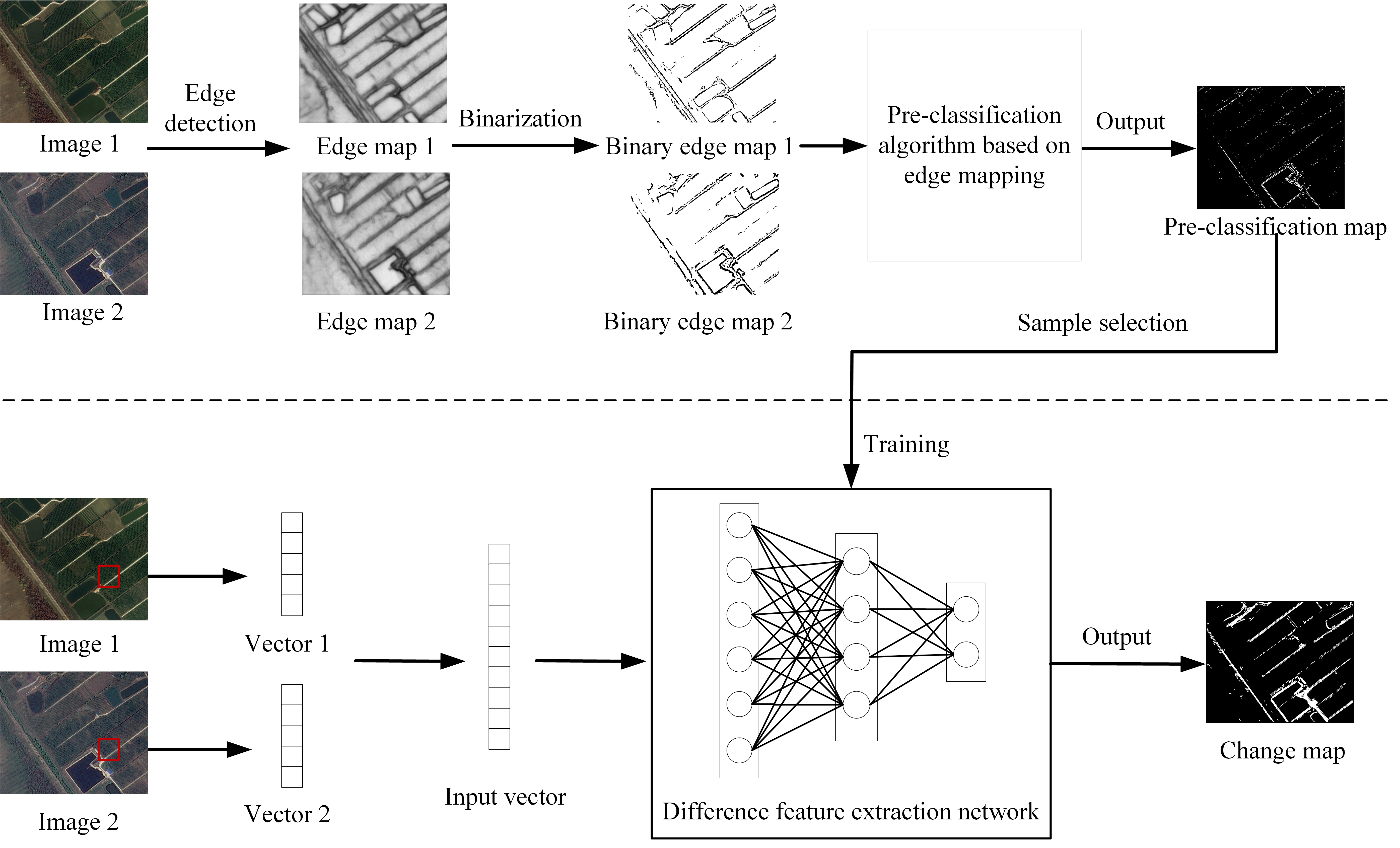
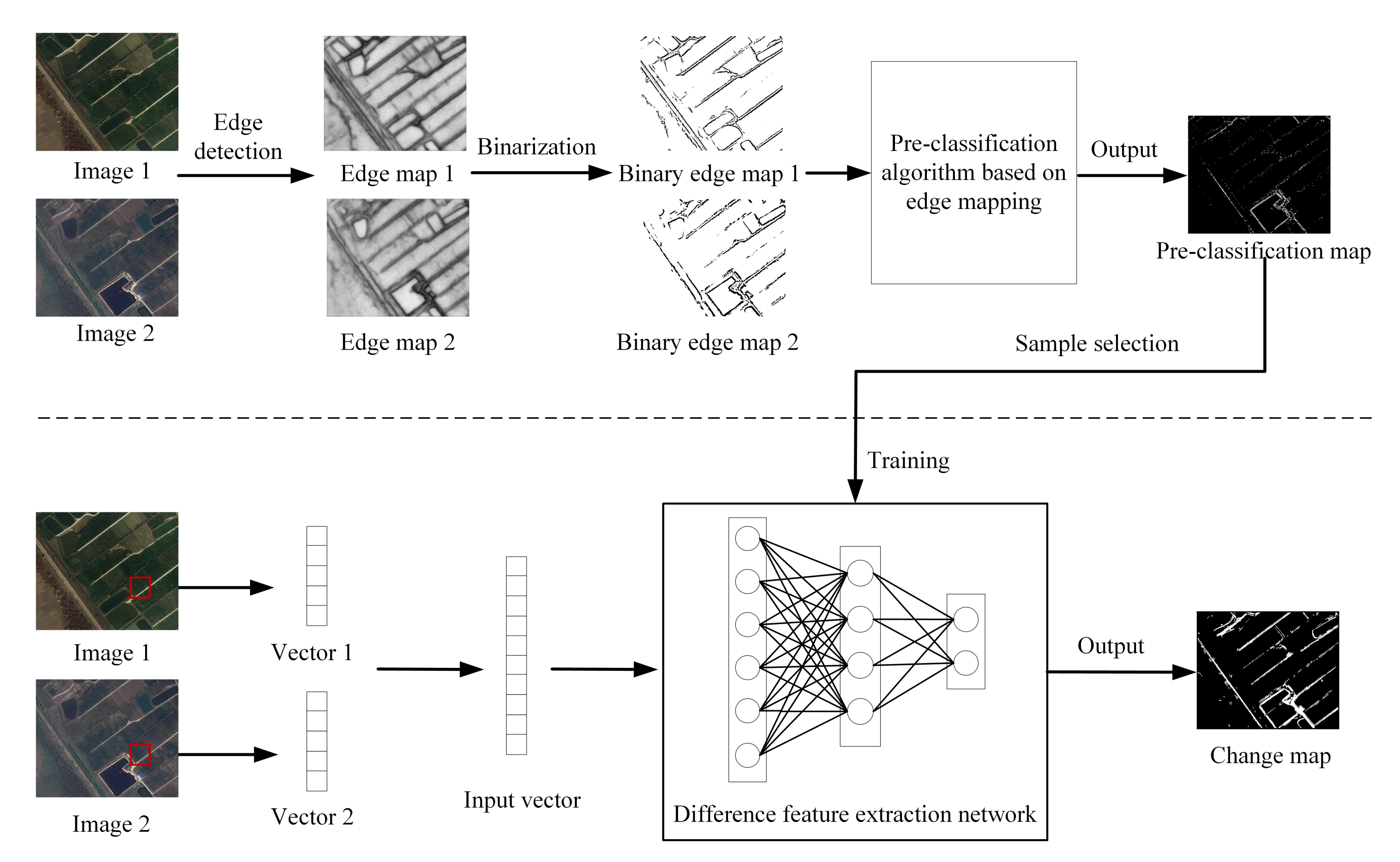
4.1. Change Detection Framework

As shown in Figure 1, the entire detection process can be divided into two stages. Each detection stage produces a change detection result, in which the pre-classification result provides the label data for the classification stage. Then, the final change map CM is obtained through the prediction of the difference extraction network.

Figure 1. The framework of the proposed change detection method.

The process of pre-classification based on edge mapping (above the dashed line in Figure 1) aims to find obvious change information through the difference of edge maps. Firstly, obtain the initial edge maps of Image1 and Image2 that refer to the co-registered $I_1$ and $I_2$. The initial edge map cannot satisfy the requirement for pre-classification, because the edge map is not a binary image but a grayscale one, which is not easy to determine the exact position of the edge. For this, the second step needs to convert the original edge map to a binary one. The third step carries out the edge maps based pre-classification algorithm. Since the areas near the inconsistent edges are considered as “changed”, the surrounding pixels in inconsistent edges are also inclined to be “changed” with a high probability, according to the continuity of changed regions. However, there are misclassified pixels in the detection results of the former stage. The noise samples in the pre-classification results will make it difficult for the neural network to accurately capture the features of difference. To achieve as high accuracy training samples as possible for the neural network, we should refine the pre-classification results in the last step.

The process of classification based on the difference extraction network (below the dashed line in Figure 1) aims to find more subtle changes. With comprehensive consideration from the spatial information of the local area, we take the neighbor of each pixel pair corresponding to the same position of the image pair as the input of the neural network. Then, to improve the ability to fit the neural network for the relationship between features of difference in the pix pair and the attribute, we design an SDAE-based neural network with multiple layers.

4.2. Pre-Classification Based on Edge Mapping

4.2.1. Image Edge Detection

Image edge is one of the most basic and momentous features of an image, which contains plenty of useful information available for pattern recognition and information extraction. To obtain as many integral edges as possible, we select [43] to complete image edge detection, which is capable of the anti-noise and the acquisition of continuous lines.

4.2.2. Image Edge Binarization

To facilitate the comparison analysis of two edge maps, we need to convert the above image edges to binary images. For this, we combine two complementary threshold processing ways to get the fine binary maps without lots of noise.

Threshold processing is used to eliminate pixels in the image above or below a certain value so as to obtain a binary image, in which black and white pixels represent edges and background respectively. To complete edge binarization, we respectively implement the simple threshold processing and adaptive threshold processing (Simple threshold processing: given a threshold between 0 and 255, a grayscale image is divided into two parts through comparing the pixel value with a threshold. Adaptive threshold processing: a grayscale image is divided into two parts according to different thresholds, and each pixel block automatically calculates the appropriate threshold.) on original edge maps, and obtain two types of binary maps $E_{meth}=meth\left(E_{ori}\right)=$ {$p_{meth}(i,j)|0\le i<H,0\le j<W$}, where $E_{ori}$ is the original edge map and $meth$ represents the threshold processing method: $simp$ or $adap$, and $p_{meth}(i,j)$ as the pixel value at the position of ($i,j$) can be formalized as follows:

$$\begin{array}{c}\hfill p_{meth}(i,j)=\left\{\begin{array}{cc}1,\hfill & \hfill edgepixels\\ 0,\hfill & \hfill backgroundpixels.\end{array}\right.\end{array}$$

(4)

The simple threshold processing can remove most of the background noise of the original grayscale edge map, but cannot determine the precise position of the edge; the adaptive threshold processing can preserve good edges, but cannot eliminate a large of background noise [44]. In this, we combine the two threshold processing. For the background region in the result of simple threshold processing, if the corresponding region in the result of adaptive threshold processing has noise, we eliminate the noise. For the non-background region, the corresponding region in the result of adaptive threshold processing keeps the same. The final binary edge map $E_{bina}$ can be formalized as follows:

$$\begin{array}{c}\hfill p_{bina}(i,j)=\left\{\begin{array}{cc}{p}_{adap}(i,j),\hfill & \hfill p_{simp}(i,j)=1\\ 0,\hfill & \hfill p_{simp}(i,j)=0,\end{array}\right.\end{array}$$

(5)

where $p_{bina}(i,j)$ represents the pixel value at position ($i,j$) in the $E_{bina}$.

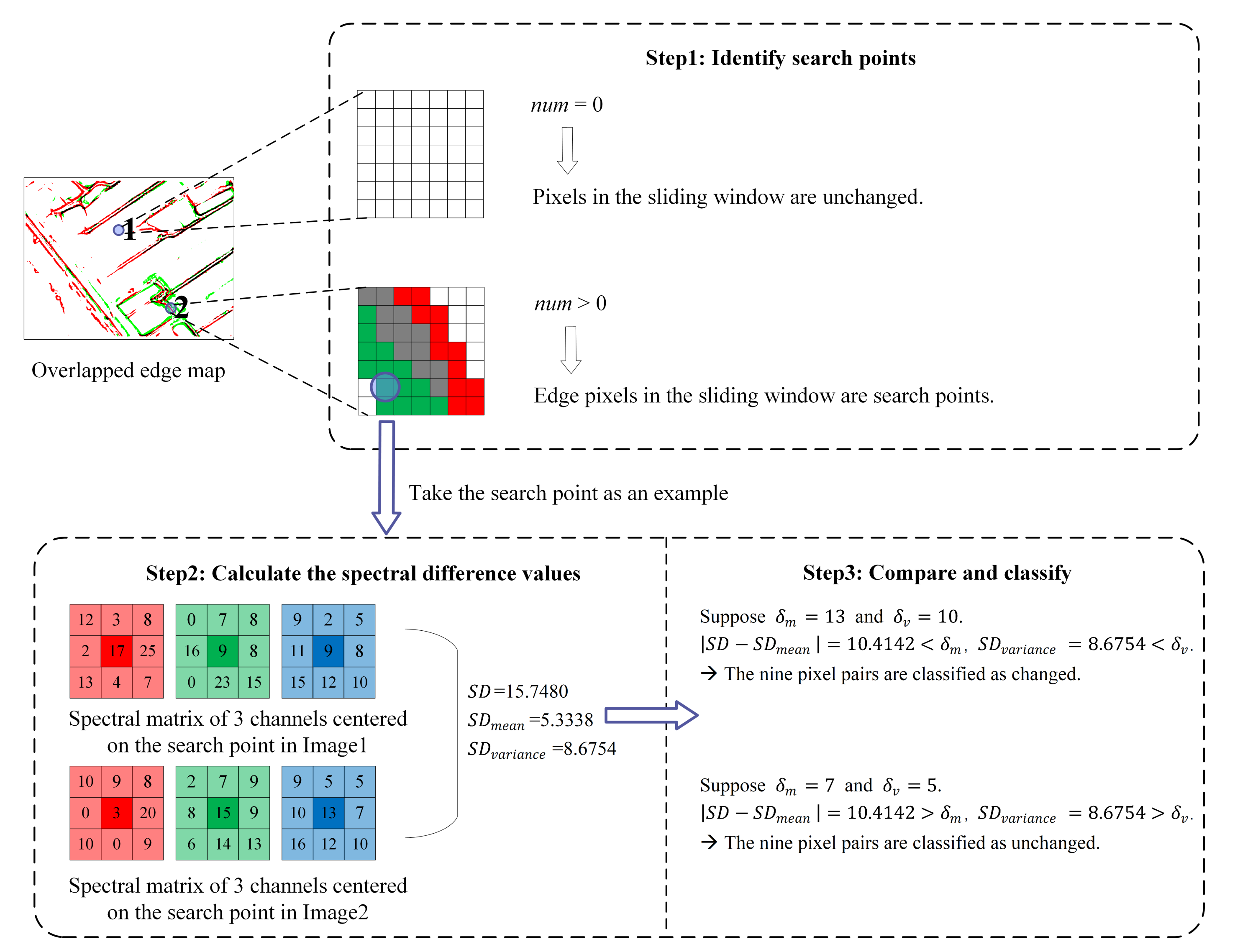
4.2.3. Pre-Classification Algorithm Based on Edge Mapping

Given two binary edge maps $E_1$ and $E_2$ of the bi-temporal images, $I_1$ and $I_2$ can be classified into two categories: changed region $R_c$ and unchanged region $R_{uc}$. To acquire the difference of $E_1$ and $E_2$, we overlap them to form an edge difference map. In this map, if there exist edges somewhere, the corresponding pixels of the image pair are likely to be changed. In the meantime, we set these pixels as the search points, and further analyze whether the surrounding pixels of search points have similar difference characteristics in $I_1$ and $I_2$. If so, the pixels around the search points are also classified as $R_c$. Otherwise, the surrounding pixels are classified as $R_{uc}$. Considering that $R_c$ is usually continuous and rarely has isolated pixels, the search points are also re-classified as $R_{uc}$.

The pre-classification algorithm can be summarized as four steps: (1) identify search points; (2) calculate the spectral difference values of the search points as well as the neighbor pixels; (3) compare and classify; (4) repeat the above steps. Firstly, we take the edge pixels in the edge difference map as the potential search points. Whereas, not all the pixels can be considered as the search points because the edge maps may contain some subtle edges detected falsely. To reduce the impact of these wrong edges, we set a sliding window to scan the edge difference map, from left to right and top to bottom. When the sliding window is scanning to a certain position, the number $num$ of edge pixels of the current window is counted. If $num$ is zero, the corresponding region of the sliding window in $I_1$ and $I_2$ is classified as $R_{uc}$. If $num$ is larger than zero, these pixels are set as the search points. Secondly, we compute the Spectral Difference (SD) values of the search-point positions in $I_1$ and $I_2$. The calculation formula is as follows:

$$SD=\sqrt[]{\sum _{c=1}^3{|p_1^c(i,j)-p_2^c(i,j)|}^2},$$

(6)

where c indicates the channels (red, green, and blue) of $I_1$ and $I_2$. Then, respectively calculate the mean $S{D}_{mean}$ and variance $S{D}_{variance}$ of the spectral difference values of eight pixels around the search point. The calculation formula is as follows:

$$S{D}_{mean}=\frac{1}{8}\sum _{n=1}^{8}S{D}_n,$$

(7)

$$S{D}_{variance}=\frac{1}{8}\sum _{n=1}^8{|S{D}_n-S{D}_{mean}|}^2,$$

(8)

where $S{D}_n$ indicates the spectral difference value of the n-th neighbor pixel. Thirdly, for comparison and classification, the surrounding pixels and search points will be classified as $R_c$ or $R_{uc}$ according to the spectral difference values of these pixels. The classification equation is as follows:

$$pixel\in \left\{\begin{array}{cc}{R}_c,\hfill & \hfill |SD-S{D}_{mean}|<{\delta }_m,andS{D}_{variance}<{\delta }_v\\ R_{uc},\hfill & \hfill otherwise,\end{array}\right.$$

(9)

where ${\delta }_m$ and ${\delta }_v$ represent the threshold of mean and variance, separately. Fourthly, repeat the above three steps until the result of pre-classification no longer changes. Besides, search-point identification is different when repeating the above steps. The search points are based on the result of the current pre-classification, not the edge difference map. This means that we compute the number of changed pixels in the current pre-classification result and further utilize the condition ($num>0$) to identify the search points. Through the above steps, we finally get PC results. The pseudocode of the algorithm is shown in Algorithm 1.

Algorithm 1 Pre-classification based on Edge Mapping

Input:$I_1$, $I_2$, $E_1$, and $E_2$

Output:$R_c$ and $R_{uc}$ 1: $/*$ Identification of search points $*/$ 2: for each $h\in [0,H]$ do 3:  for each $w\in [0,W]$ do 4:   Set a sliding window centered at the pixel of $(h,w)$; 5:   Count the number $num$ of edge pixels in the sliding window; 6:   if$num$= 0 then 7:    Pixels in the sliding window ∈$R_{uc}$; 8:   else 9:    Edge pixels are set as search points; 10:   end if 11:  end for 12: end for 13: /* Computation of spectral difference value */ 14: for each $pixel\in$ search points do 15:  Compute the spectral difference value $SD$ of $pixel$ and $S{D}_n$ of the neighbor pixels; 16:  /* Comparison and classification */ 17:  if$|SD-S{D}_{mean}|$<${\delta }_m$ and $S{D}_{variance}$<${\delta }_v$ then 18:   $pixel$ and the neighbor ∈$R_c$; 19:  else 20:   $pixel$ and the neighbor ∈$R_{uc}$; 21:  end if 22: end for 23: /* Repeat until the pre-classification result keeps the same */

As shown in Figure 2, we give an example to visually show the pre-classification process of pixel pairs. In the overlapped edge map, red pixels and green pixels represent the edge of $I_1$ and $I_2$, and the black pixels represent their common edges. In the sliding window 1, num is 0, so the pixels in the sliding window are classified into $R_{uc}$. In the sliding window 2, num is larger than 0, so the edge pixels in the sliding window are identified as search points. Next, take the edge pixels surrounded by the blue circle as an example. We calculate the spectral difference value of the search point, as well as the mean and variance of the spectral difference values of the neighbor pixels. The spectral matrixes of red, green, and blue channels centered on the search point in $I_1$ and $I_2$ are assumed as in Figure 2. Through calculation, $SD$, $S{D}_{mean}$, and $S{D}_{variance}$ are 15.7480, 5.3338, and 8.6754, respectively. Then, we give two hypotheses (To facilitate readers to understand the calculation process of Step 3 (compare and classify), the values of ${\delta }_m$ and ${\delta }_v$ here are hypothetical and do not represent their actual values.): (1) ${\delta }_m=13$, ${\delta }_v=10$; (2) ${\delta }_m=7$, ${\delta }_v=5$. We classify the search point and the neighbor after comparing the relationship between $|SD-S{D}_{mean}|$ and ${\delta }_m$, as well as $S{D}_{variance}$ and ${\delta }_v$.

Figure 2. An example for pre-classification. (1) count the number of edge pixels in the sliding window to identify search points; (2) calculate the spectral difference values of the search point and the neighbor pixels; (3) compare and classify according to ${\delta }_m$ and ${\delta }_v$.

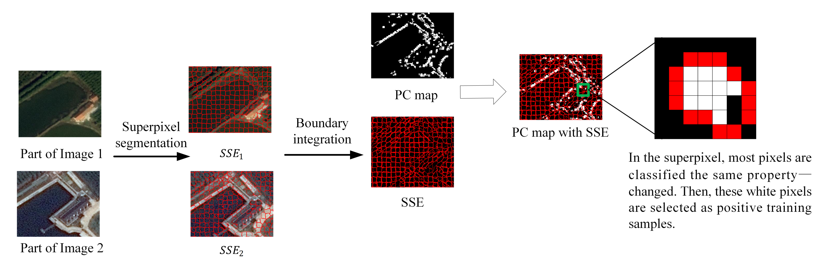
4.2.4. Sample Selection

The high-quality training samples are essential for fine-tuning the difference extraction network. Nevertheless, PC results are not completely correct because of the complexity of remote sensing images. To reduce the influence of incorrect results on the latter change detection stage, we design and apply a rule based on superpixel segmentation to select training samples. Note that there is no manual intervention in the process of sample selection.

SLIC, that is, simple linear iterative clustering, is one of the most superior superpixel segmentation algorithms, which was proposed by Achanta et al. [45]. SLIC can generate uniform compact superpixels and attach the edges of the image, which has a high comprehensive evaluation in terms of operation speed, object contour retention, superpixel shape, and so on. The superpixel refers to an irregular pixel block that is composed of adjacent pixels in one image with similar texture, color, and brightness. Therefore, there is a high probability that pixels within the same superpixel have the same change properties. Based on this, we choose more accurate parts from PC results. As shown in Figure 3, We perform superpixel segmentation on high-resolution images and obtain Superpixel Segmentation Edges $SS{E}_i(i=1or2)$. Then, PC results are divided via $SS{E}_i$. However, the content of the two remote sensing images is not completely the same since they are taken at different times, so the two superpixel segmentation edges are not consistent. We need to further fuse $SS{E}_i$ to obtain a consistent SSE to divide PC results [46]. For any superpixel, if the pixel classification results are basically the same (that is, the pixels that are determined to be changed or unchanged exceed a certain proportion of the size of the superpixel), it will be selected as training samples. The selected samples are formulated as follows:

$$\begin{array}{cc}\hfill Sample& =\{p_t(i,j)\in superpixel\left(s\right)|n_c>k_c{n}_s\wedge attr(i,j)=1\}\hfill \\ \hfill & \cup \{p_t(i,j)\in superpixel\left(s\right)|n_{uc}=k_{uc}{n}_s\},\hfill \end{array}$$

(10)

where $superpixel\left(s\right)$ represents the s-th superpixel, and $n_c$ and $n_{uc}$ indicate the number of the changed and unchanged pixels in the s-th superpixel. $n_s$ represents the total amount of the s-th superpixel. According to the rules for selecting samples, we set $k_{uc}$ to 1. When all pixels in one superpixel are classified as unchanged, we select the superpixel as negative training samples (i.e., unchanged samples). However, there are fewer changed pixels in PC results, since the changed region is usually in a small proportion. Therefore, the negative sample size is much larger than the positive sample size (i.e., changed samples), which will lead to a poor final change map. To make the positive and negative samples as balanced as possible, we slightly lower the value of $k_c$ and set it to 0.8.

Figure 3. The diagram of sample selection.

4.3. Classification Based on Difference Extraction Network

In this paper, a deep neural network based on SDAE is established. The structure of the constructed network N is shown in Figure 4. Next, we introduce the conversion of remote sensing images to the input of the neural network, the structure of the neural network, and the training process.

Figure 4. The structure of difference extraction network.

Remote sensing images cannot be used as the input of the neural network directly, which requires transformation. As shown in Figure 4a, $B_t(i,j)$ represents a pixel block that is centered at the pixel of the position $(i,j)$ in the image acquired in time $t(t=1or2)$. Here, we take the pixel block but not a single pixel as an analysis unit because the surroundings of a pixel can provide some spatial and texture information. Then, $B_t(i,j)$ of two images are vectorized into two vectors $V_t(i,j)$. Finally, the two vectors are stacked together to be the input of the neural network. Note that the final classification result by the neural network is the result of the central pixel.

The difference extraction network has input, hidden, and output layers, in which the hidden layers are constituted by SDAE. SDAE is a main unsupervised model in deep learning, with the function of reducing noise and extracting robust features. As shown in Figure 4b, SDAE is a stack of multiple Denoising Auto-Encoders (DAE). DAE is developed from Auto-Encoder (AE) [47]. The following will start from AE, and gradually transition to SDAE. Given the input vector x $\in {[0,1]}^d$, the input is first encoded with the encoder function y = $f_{\theta }$ (x) = h (Wx + b) to obtain the hidden value y$\in {[0,1]}^{d^{’}}$, and $\theta$ = {W, b}. Then the decoder function x’ = $g_{{\theta }^{’}}$ (y) = h (W’ y + b’) is used to decode y to obtain x’ and ${\theta }^{’}$ = {W’, b’}. Through repeatedly training, the parameters (i.e., $\theta ,{\theta }^{’}$) are optimized and the reconstruction error is reduced gradually. Finally, x is approximated to x’. To extract more robust features from the input data, DAE takes a broken variant of x (written as $\tilde{\mathit{x}}$ ) as input and z as the output. After reducing the reconstruction error (note that the reconstruction error is the difference between z and x, not between z and $\tilde{\mathit{x}}$), z is getting closer to x. That is, DAE can reconstruct the original data from the broken data. Multiple DAEs can be stacked to form SDAE with a certain depth [48].

The number of neurons in the hidden layers of the network is designed in three cases (viz., Section 5.3). To prevent overfitting, we use a $dropout$ strategy for neurons in the input layer with a dropout rate of 0.1 [49]. Furthermore, in order to decrease the influence of Gaussian noise on the change detection result, we also add the Gaussian distribution noise to the input x, so that trained SDAE can extract the abstract features and eliminate Gaussian noise in the remote sensing images.

The whole neural network needs to be trained to have a good ability to extract complex features of difference, thereby detecting more subtle changes. Its training is divided into two parts: unsupervised pre-training of SDAE and supervised fine-tuning of the whole network. In the pre-training phase of SDAE, the training pattern is layer by layer. After the former DAE is trained completely, its hidden layer is used as the input of the next DAE, and so on until all DAEs are trained. Moreover, the parameters $\theta$ and ${\theta }^{’}$ of this model are optimized to minimize the average reconstruction error after finishing training, as follows:

$$\begin{array}{cc}\hfill {\theta }^{*},{\theta }^{’*}& =argmin\frac{1}{n}\sum _{i=1}^{n}L(x^{\left(i\right)},z^{\left(i\right)})\hfill \\ \hfill & =argmin\frac{1}{n}\sum _{i=1}^{n}L(x^{\left(i\right)},g_{{\theta }^{’}}(f_{\theta }({\tilde{x}}^{\left(i\right)}))),\hfill \end{array}$$

(11)

where L is a loss function that represents the reconstruction error between x and z. Here, we use traditional squared error as the loss function, which is defined as follows:

$$L(\mathbf{x},\mathbf{z})=\left|\right|\mathbf{x}-{\mathbf{z}\left|\right|}^2.$$

(12)

In the fine-tuning stage, some relatively reliable pixel pair samples selected from PC results are employed to train the network in a supervised way, so that the network can efficiently mine the abstract features of difference in the image pair. We use the $Adamoptimizer$ to continuously reduce the loss function. For the binary classification problem, we use binary cross entropy as the loss function, which is defined as follows:

$$L(\widehat{y},y)=-ylog\widehat{y}-(1-y)log(1-\widehat{y}),$$

(13)

where y represents the label of training samples, and $\widehat{y}$ represents the prediction value of the neural network.

5. Experimental Studies

In this section, we firstly describe the experimental setup. Next, we discuss the range of parameters in the process of pre-classification is through multiple experiments and evaluate the results of the pre-classification quantitatively. At last, we evaluate the performance of classification by implementing several groups of comparison experiments with other methods.

5.1. Experimental Setup

We describe the datasets used in our experiment, the evaluation indicators for the change detection results, as well as the comparison methods below. The brief summary is shown in Table 1.

Table 1. Brief summary of datasets, criteria and comparison methods.

Datasets description	Dataset	Size	Spatial resolution	${\mathit{t}}_1$	${\mathit{t}}_2$	Region
	Farmland Dataset	$1502\times 1908$	0.3 m	2009	2013	Huaxi Village, Chongming District, Shanghai, China
	Forest Dataset	$503\times 878$	0.3 m	2011	2015	Wenzhou City, Zhejiang Province, China
	Weihe Dataset	$1913\times 2821$	0.3 m	2014	2017	Tongguan County, Weinan City, China
Evaluation criteria	Criteria	Description
	FA	The proportion of pixels in the change map that are misjudged as changed
	MA	The proportion of pixels in the change map that are actually change but are not detected
	OE	The overall error rate, which is the sum of FA and MA
	CA	The proportion of pixels in the change map that are classified correctly
	KC	The degree of similarity between the change map and the ground truth
Comparison methods	IR-MAD [27]	The iteratively reweighted multivariate alteration detection method for change detection
	PCA-k-means [15]	Unsupervised change detection method using principal component analysis and k-means clustering
	CaffeNet [25]	A novel deep Convolutional Neural Networks features based change detection method
	USFA [28]	Slow feature analysis algorithm based change detection method
	DSFA [26]	Unsupervised change detection method based on deep network and slow feature analysis theory

Datasets description: the first dataset is the Farmland Dataset. As shown in Figure 5, the main changes in the image pair are the increase in the structure. The second is the Forest Dataset, and the main changes in the image pair are that portions of the forest have been converted into roads. The illustration is shown in Figure 6. The third dataset is the Weihe Dataset. As shown in Figure 7, the image content is water area, roads, buildings, farmland, etc. The main changes are the water area freezing and the augment of lots of buildings. The above three datasets are downloaded from the website shuijingzhu where the high-resolution remote sensing images are sourced from Google Earth [50]. The ground truth of three datasets is derived from the real world and manual experience. Then, they are achieved using software $envi$ and $labelme$ [51,52].

Figure 5. Farmland Dataset.

Figure 6. Forest Dataset.

Figure 7. Weihe Dataset.

Evaluation criteria: there are many evaluation indicators in remote sensing image change detection, which can reflect the performance of various methods from different aspects. We adopt False Alarm rate (FA), Missed Alarm rate (MA), Overall Error rate (OE), Classification Accuracy (CA), and Kappa Coefficient (KC) as evaluation criteria. Given a binary change detection map, the black areas represent “unchanged” and the white areas represent “changed”. Then, the above evaluation indicators are calculated as follows:

$$FA=\frac{FP}{(TP+TN+FP+FN)},$$

(14)

$$MA=\frac{FN}{(TP+TN+FP+FN)},$$

(15)

where $TP$ denotes the number of pixels that are predicted to be changed and actually have changed, $TN$ indicates the number of pixels that are unchanged in the actual and prediction, $FP$ represents the number of pixels that are not actually changed but are predicted as changed, and $FN$ represents the number of pixels that are actually changed but are predicted to be unchanged.

$$OE=FA+MA,$$

(16)

$$CA=\frac{TP+TN}{TP+TN+FP+FN},$$

(17)

$$KC=\frac{CA-PRE}{1-PRE},$$

(18)

$$PRE=\frac{(TP+FP)·N_{pos}+(FN+TN)·N_{neg}}{{(TP+TN+FP+FN)}^2},$$

(19)

where $N_{pos}$ and $N_{neg}$ indicate the changed and unchanged pixels in the ground truth separately.

Comparison methods: to verify the high efficiency of the proposed method, we choose traditional unsupervised methods (IR-MAD, PCA-k-means, CaffeNet, USFA, and DSFA) to compare with our method [15,25,26,27,28].

5.2. Pre-Classification Evaluation

In the pre-classification algorithm, there are three variable parameters: ${\delta }_m$, ${\delta }_v$, and the $size$ of the sliding window. For the purpose of studying the influence of these parameters on the results of pre-classification, we conduct multiple sets of comparison experiments to find the appropriate range of the parameters. Moreover, the superpixel area in the SLIC algorithm also has a certain impact on the results of sample selection. We also perform an experimental analysis of this parameter. Here, we use the Classification Accuracy (CA), Classification Precision (CP) (Classification Precision = $TP/(TP+FP)$), and Classification Recall (CR) (Classification Recall = $TP/(TP+FN)$) to evaluate the performance of pre-classification and sample selection under different parameter values.

Parameter${\delta }_m$: in the analysis of ${\delta }_m$, we set ${\delta }_v$ and $size$ to 0.01 and 7, respectively, and experiment with ${\delta }_m$ in the range of 0.06 to 0.2. The experimental results of the three datasets are shown in Figure 8. As ${\delta }_m$ increases, both CA and CP in the pre-classification results increase, while CR decreases. Moreover, three indicators are all basically stable when ${\delta }_m$ is larger than 0.1. For the training of the later neural network, CP of positive samples is very important, so we try to choose one value for ${\delta }_m$ that makes CP in the pre-classification results higher. Here, we set ${\delta }_m$ to 0.1 for three datasets.

Figure 8. Relationship between parameter ${\delta }_m$ and the result of pre-classification.

Parameter${\delta }_v$: for the analysis of ${\delta }_v$, we set ${\delta }_m$ and $size$ to 0.1 and 7, and select the experimental range of (0.006, 0.02) for ${\delta }_v$. The experimental results of the three datasets are shown in Figure 9. With the increase of ${\delta }_v$, CA and CP have the same trend as that of ${\delta }_m$ that increase roughly. Nevertheless, CR has been decreasing when ${\delta }_v$ is in the range (0.006, 0.02). Correspondingly, the number of correctly classified pixels in the actual changed region will be reduced. This will result in too few positive training samples available for the neural network to learn the features of difference in the two remote sensing images. To ensure sufficient and high accuracy samples, we set ${\delta }_v$ to 0.01 for three datasets.

Figure 9. Relationship between parameter ${\delta }_v$ and the result of pre-classification.

Parameter$size$: combining the analysis for the first two parameters, here we set ${\delta }_m$ and ${\delta }_v$ to 0.1 and 0.01, respectively, and experiment with $size$ on seven values of 3, 5, 7, 9, 11, 13, and 15. As shown in Figure 10, with the increase in $size$, CA and CP basically show a downward trend and CR gradually rises. For $size$, we use a strategy to determine its value depending on ${\delta }_m$ and ${\delta }_v$. In Figure 8 and Figure 9, we finally set ${\delta }_m$ and ${\delta }_v$ to 0.1 and 0.01 when CR floats above and below 0.08. We also determine the value of $size$ when CR is 0.08. In the Farmland Dataset, CR is closest to 0.08 when $size$ is 7. Similarly, the value of $size$ is 5 and 15 in the Forest and Weihe Dataset separately.

Figure 10. Relationship between parameter $size$ and the result of pre-classification.

Parameter$superpixelarea$: we set $superpixelarea$ to 10, 20, 30, 40, 50, 60, 70, 80, 90, and 100, in which $superpixelarea$ refers to the number of pixels in one superpixel. The experimental results of the three Datasets are shown in Figure 11. Note that when the abscissa of $superpixelarea$ is pre, the ordinate represents the evaluation of original pre-classification. As $superpixelarea$ increases, CA is relatively stable with a small increase; CP generally has a large increase; and CR continues to decrease. When $superpixelarea$ is 50, CP in the three datasets is relatively high, and CA and CR are at an intermediate level under ten different values. Therefore, we set $superpixelarea$ as 50 when CA and CP of the selected samples are higher and the sample size is enough to train the neural network.

Figure 11. Relationship between parameter $superpixelarea$ and the result of sample selection.

Moreover, Table 2 shows the pre-classification accuracy and precision of three datasets before and after sample selection, as well as the number of positive and negative samples used for training neural networks. It can be seen from Table 2 that the quality of the sample is superior and the amount of the sample is enough large. Sample selection does further improve the accuracy and precision of pre-classification.

Table 2. Quantitative results of pre-classification of three datasets.

Dataset	Before Sample Selection			After Sample Selection
	Farmland	Forest	Weihe	Farmland	Forest	Weihe
Acuuracy	0.8938	0.7246	0.7182	0.9385	0.8229	0.7057
Precision	0.5770	0.5412	0.3148	0.6994	0.5615	0.3573
Positive sample number	-	-	-	7077	894	111636
Negative sample number	-	-	-	2,374,299	174,379	2,971,483

5.3. Classification Evaluation

We firstly elaborate on the experimental settings. Then, we use three datasets to compare with other methods to evaluate the classification performance of the neural network. Next, we study the influence of pre-training on change detection and the influence of the size of the pixel block $blocksize$ by carrying out multiple experiments.

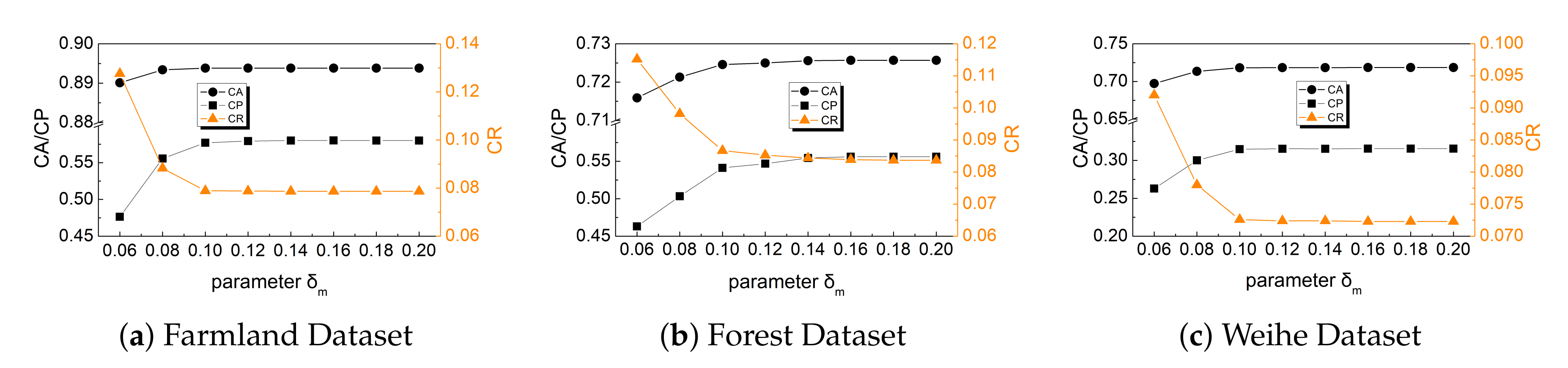
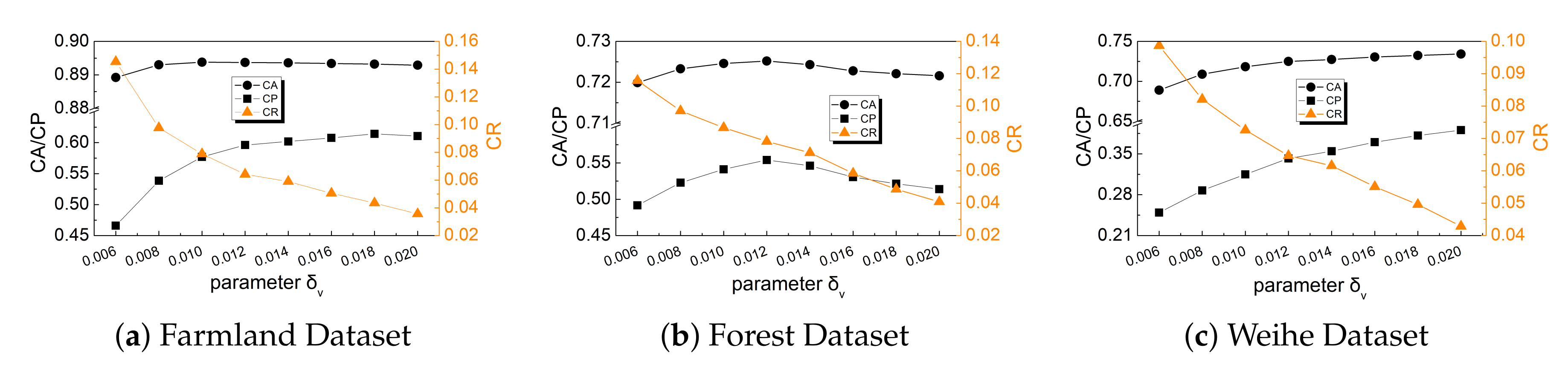
5.3.1. Experimental Settings

We designed three network structures of hidden layers: 100-50-20, 200-100-50-20, and 500-200-100-50-20 (In $l_1-l_2-l_3-\dots -l_n$, $l_i$ represents the number of neuron in i-th layer.). For the input layer of the neural network, we designed two cases of using dropout with a rate of 0.1 and not using dropout. That is, we designed six types of neural network structures and would analyze the detection results in each case. The weights and biases of the whole neural network are initialized randomly. Meanwhile, the network is pre-trained via unsupervised feature learning to obtain a good initialization to facilitate the subsequent backpropagation algorithm. In the backpropagation stage, the training set is part of the pre-classification results, and the test set is the entire remote sensing image to be detected. In addition, to reflect the performance of our proposed method as authentically as possible, our change detection results below are the average of 10 repeated experiments. In the stage of supervised training, we randomly undersample the positive samples to make the total of positive and negative samples the same since the negative samples are much more than the positive samples.

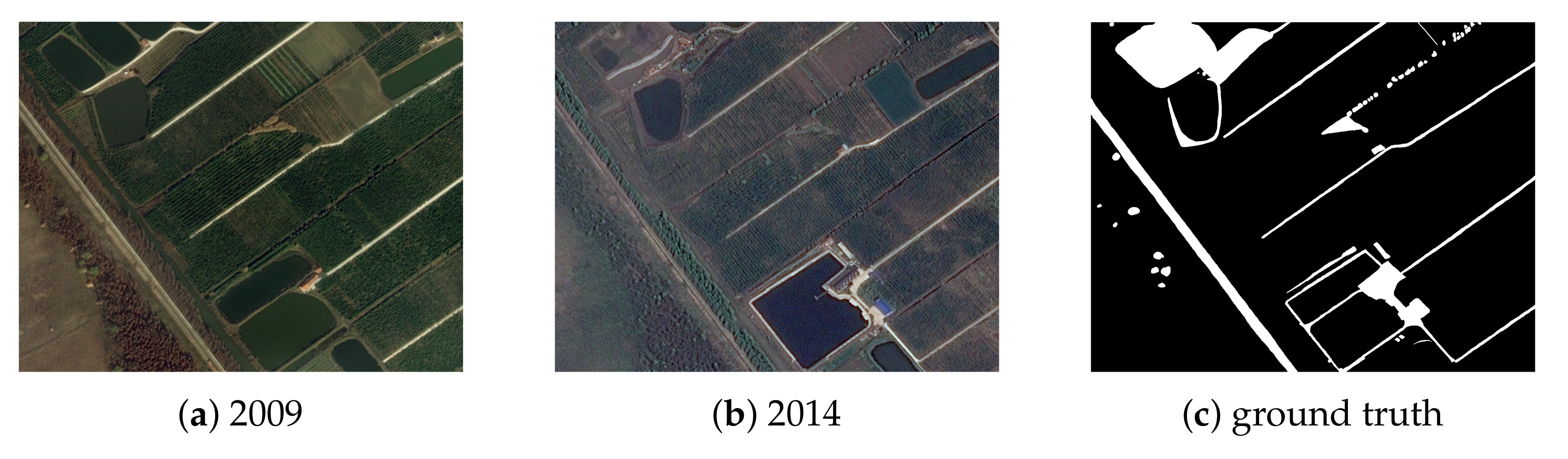
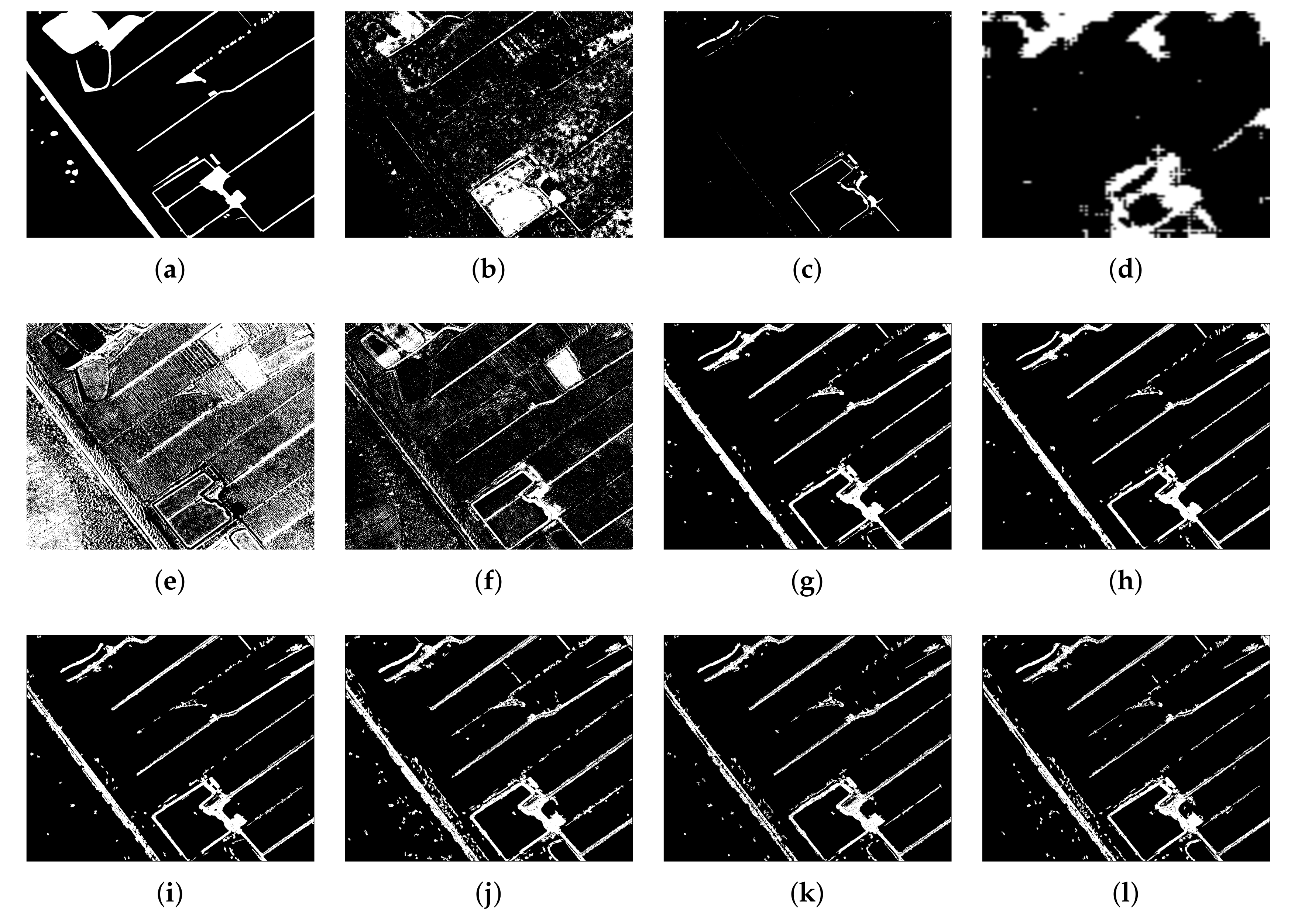
5.3.2. Results of the Farmland Dataset

As shown in Figure 12, (a) is the ground truth of the Farmland Dataset, (b)–(f) are the results of several comparison methods, and (g)–(l) are the results of our proposed method under different parameters. It can be seen from the figure that the result of IR-MAD, USFA, and DSFA has more noise, i.e., white spots. PCA-k-means could effectively remove most of the noise, but it cannot detect part of changed areas. On the contrary, although CaffeNet gets out noises, the changed area detected is not precise enough. Our method can alleviate such a problem to some extent. The results of EM-SDAE not only have rare isolated white speckle noise but also detect most of the changed regions. Although (g)–(l) are the results of EM-SDAE under different network structures, the important changes are basically the same. The main difference between these change maps is the number of white spots.

Figure 12. Change detection results of the Farmland Dataset. (a) Ground truth; (b) IR-MAD; (c) PCA-k-means; (d) CaffeNet; (e) USFA; (f) DSFA; (g) EM-SDAE: 100-50-20/with dropout; (h) EM-SDAE: 200-100-50-20/with dropout; (i) EM-SDAE: 500-200-100-50-20/with dropout; (j) EM-SDAE: 100-50-20/no dropout; (k) EM-SDAE: 200-100-50-20/no dropout; (l) EM-SDAE: 500-200-100-50-20/no dropout.

In order to quantify the experimental results of several methods on the Farmland Dataset, Table 3 shows the specific values of FA, MA, OE, CA, and KC. Due to the influence of noise, USFA has the highest FA. Although PCA-k-means has almost removed all white noise spots, it cannot detect some relatively weak changed areas. Thus, its MA is the highest. Both FA and MA of our method are at a better level, so CA and KC are the highest. As can be seen from the table, using dropout in the input layer brings better results, when the hidden layers of the neural network are the same. Regardless of whether dropout is used or not, the different structures of hidden layers in the neural network have little effect on the final result and the performance is relatively stable.

Table 3. Quantitative comparison of the Farmland Dataset with other methods.

Different Methods	FA	MA	OE	CA	KC
IR-MAD	0.1194	0.0667	0.1861	0.8139	0.2068
PCA-k-means	0.0006	0.0959	0.0965	0.9035	0.1506
CaffeNet	0.0506	0.0565	0.1070	0.8930	0.3227
USFA	0.3975	0.0585	0.4560	0.5440	0.0062
DSFA	0.0909	0.0491	0.1400	0.8600	0.3813
EM-SDAE:100-50-20/with dropout	0.0410	0.0509	0.0919	0.9081	0.5054
EM-SDAE:200-100-50-20/with dropout	0.0345	0.0537	0.0882	0.9118	0.5059
EM-SDAE:500-200-100-50-20/with dropout	0.0342	0.0547	0.0889	0.9111	0.4991
EM-SDAE:100-50-20/no dropout	0.0531	0.0504	0.1035	0.8965	0.4708
EM-SDAE:200-100-50-20/no dropout	0.0360	0.0595	0.0955	0.9045	0.4546
EM-SDAE:500-200-100-50-20/no dropout	0.0376	0.0563	0.0939	0.9061	0.4750

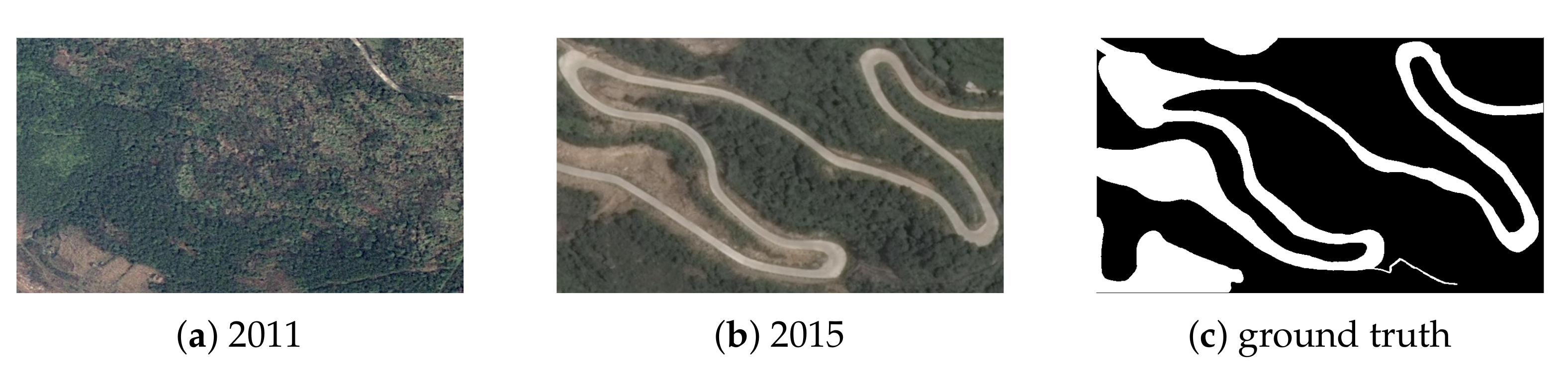
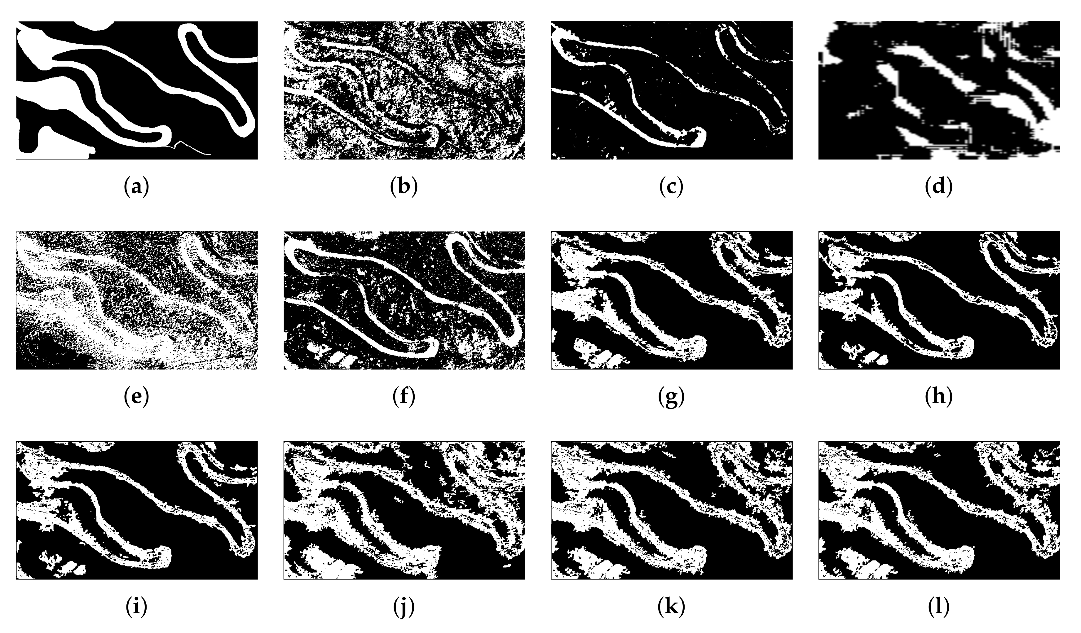
5.3.3. Results of the Forest Dataset

The experimental results of our proposed method and other comparison methods are shown in Figure 13. The main content of the Forest Dataset is a mass of trees, which shows different color distributions in different seasons. Judging from the result of IR-MAD and USFA that has much more white noise spots, they detect some seasonal changes in the forest and differences in light. In contrast, PCA-k-means, CaffeNet, DSFA, and EM-SDAE is more inclined to detect obvious changes and is less susceptible to factors such as light and atmosphere. (g)–(l) show that the results of EM-SDAE almost have no white spots and it detects changes in multiple areas in the Forest Dataset. As shown in Figure 14, we exhibit some feature images extracted from the third hidden layer under the network structure of (100-50-20). It is clear that the neral network is able to learn meaningful features and overcome the noise. A hidden layer could obtain different feature images, which have different representations. This demenstrates EM-SDAE can represent the difference features of the two remote sensing images.

Figure 13. Change detection results of the Forest Dataset. (a) Ground truth; (b) IR-MAD; (c) PCA-k-means; (d) CaffeNet; (e) USFA; (f) DSFA; (g) EM-SDAE: 100-50-20/with dropout; (h) EM-SDAE: 200-100-50-20/with dropout; (i) EM-SDAE: 500-200-100-50-20/with dropout; (j) EM-SDAE: 100-50-20/no dropout; (k) EM-SDAE: 200-100-50-20/no dropout; (l) EM-SDAE: 500-200-100-50-20/no dropout.

Figure 14. Feature images of Forest Dataset extracted from different neurons of the third layer. (a) feature image from the 1st neuron; (b) feature image from the 3rd neuron; (c) feature image from the 5th neuron; (d) feature image from the 7th neuron; (e) feature image from the 9th neuron; (f) feature image from the 11th neuron; (g) feature image from the 13th neuron; (h) feature image from the 15th neuron; (i) feature image from the 17th neuron; (j) feature image from the 19th neuron.

From Table 4, CA and KC of our method are the highest, indicating that our classification results are most consistent with the ground truth. Similarly, it is better to detect changes when the input layer of neural networks uses dropout. The different structures of the neural networks have a greater impact on the final result when dropout is not used.

Table 4. Quantitative comparison of the Forest Dataset with other methods.

Different Methods	FA	MA	OE	CA	KC
IR-MAD	0.2712	0.1498	0.4210	0.5790	0.0768
PCA-k-means	0.0181	0.1590	0.1771	0.8229	0.4792
CaffeNet	0.0670	0.2057	0.2728	0.7272	0.1823
USFA	0.3316	0.0759	0.4075	0.5925	0.2092
DSFA	0.1003	0.1325	0.2327	0.7673	0.4413
EM-SDAE:100-50-20/with dropout	0.0668	0.0790	0.1458	0.8542	0.6326
EM-SDAE:200-100-50-20/with dropout	0.0387	0.1050	0.1437	0.8563	0.6148
EM-SDAE:500-200-100-50-20/with dropout	0.0436	0.0869	0.1305	0.8695	0.6594
EM-SDAE:100-50-20/no dropout	0.1680	0.0651	0.2331	0.7669	0.4794
EM-SDAE:200-100-50-20/no dropout	0.1199	0.0617	0.1816	0.8184	0.5759
EM-SDAE:500-200-100-50-20/no dropout	0.1093	0.0615	0.1708	0.8292	0.5967

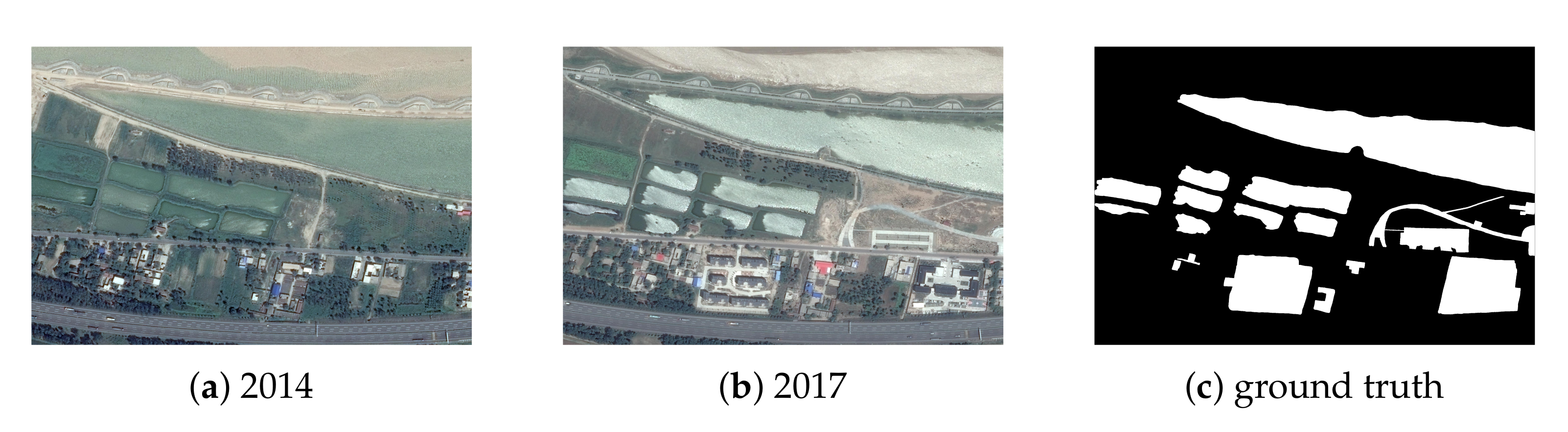
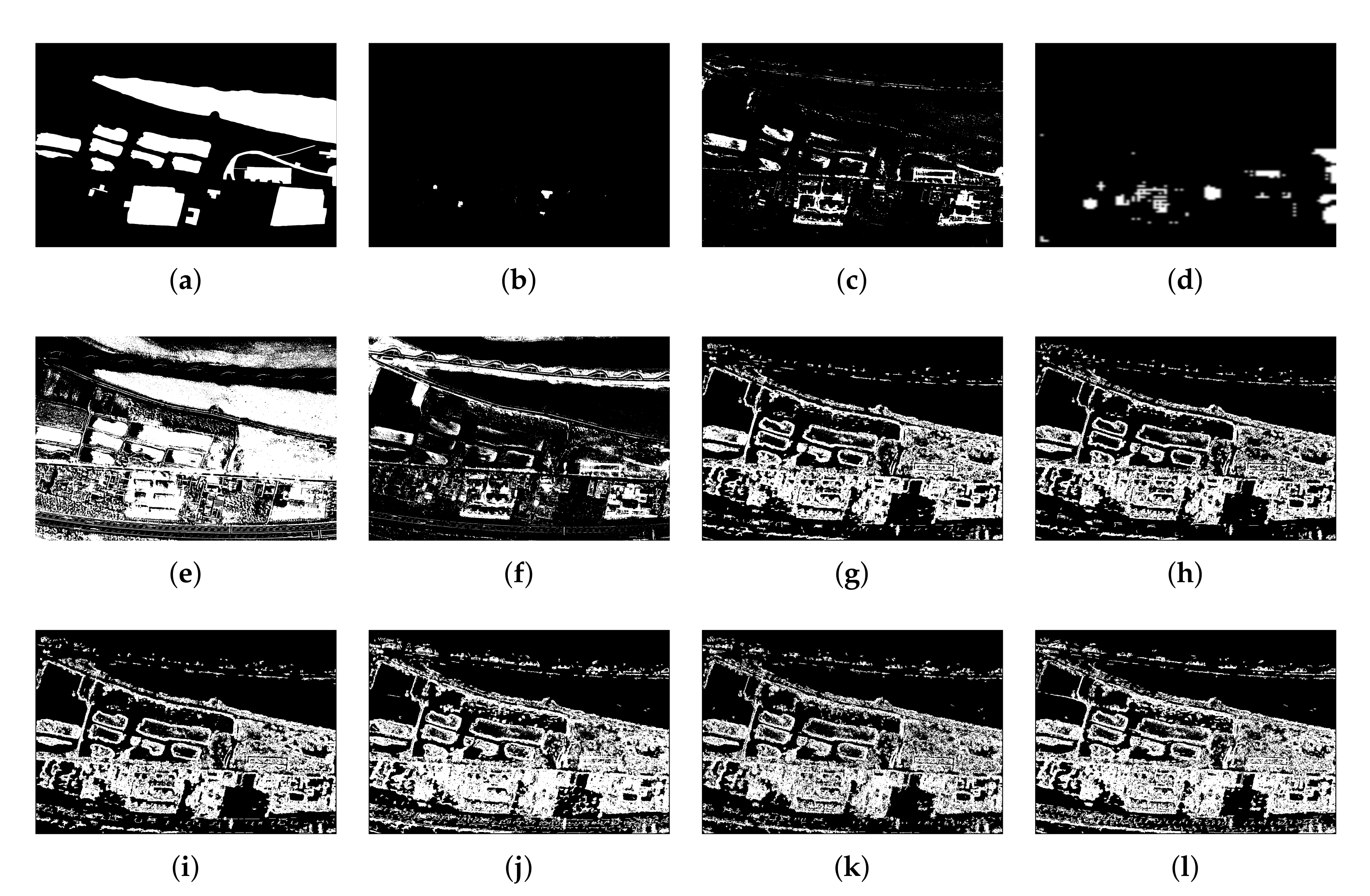
5.3.4. Results of the Weihe Dataset

Compared to the Farmland and Forest Dataset, the Weihe Dataset contains more detailed texture information, and the detection difficulty increases accordingly. As shown in Figure 15, (b)–(l) are the results of several comparison methods and EM-SDAE under different parameters. IR-MAD and CaffeNet methods can hardly detect the changed areas of the Weihe Dataset. So their KC is relatively low. DSFA also cannot detect most of changed areas but detects some ‘false’ changed parts. Compared with Figure 7a, a large number of green plants have withered and decayed in Figure 7b. EM-SDAE detects this vegetation replacement phenomenon as changed, so it has a higher FA. PCA-k-means focuses on identifying meaningful changes and has a lower FA, which ultimately leads to CA and KC higher than EM-SDAE. Moreover, part of the water area in Figure 7b is frozen, while EM-SDAE fails to detect the changes between the different forms of water. Although there are many noises in the result of USFA, almost all the changes are detected. So USFA performs best in the Weihe Dataset.

Figure 15. Change detection results of the Weihe Dataset. (a) Ground truth; (b) IR-MAD; (c) PCA-k-means; (d) CaffeNet; (e) USFA; (f) DSFA; (g) EM-SDAE: 100-50-20/with dropout; (h) EM-SDAE: 200-100-50-20/with dropout; (i) EM-SDAE: 500-200-100-50-20/with dropout; (j) EM-SDAE: 100-50-20/no dropout; (k) EM-SDAE: 200-100-50-20/no dropout; (l) EM-SDAE: 500-200-100-50-20/no dropout.

As shown in Table 5, KC of USFA is the highest, followed by PCA-k-means. Both CA and KC of our method are lower than PCA-k-means and USFA in the Weihe Dataset. In addition, using dropout is still better than not using, and the neural network structure has little effect on the final result.

Table 5. Quantitative comparison of the Weihe Dataset with other methods.

Different Methods	FA	MA	OE	CA	KC
IR-MAD	0.0002	0.2586	0.2585	0.7415	0.0083
PCA-k-means	0.0160	0.2084	0.2245	0.7758	0.2314
CaffeNet	0.0060	0.2391	0.2451	0.7549	0.0189
USFA	0.2693	0.0259	0.2952	0.7048	0.4112
DSFA	0.1238	0.1980	0.3218	0.6782	0.0770
EM-SDAE:100-50-20/with dropout	0.1726	0.1685	0.3410	0.6590	0.1173
EM-SDAE:200-100-50-20/with dropout	0.1621	0.1750	0.3370	0.6630	0.1088
EM-SDAE:500-200-100-50-20/with dropout	0.1777	0.1696	0.3473	0.6527	0.1056
EM-SDAE:100-50-20/no dropout	0.2343	0.1550	0.3894	0.6106	0.0785
EM-SDAE:200-100-50-20/no dropout	0.1884	0.1687	0.3571	0.6429	0.0933
EM-SDAE:500-200-100-50-20/no dropout	0.2233	0.1604	0.3838	0.6162	0.0745

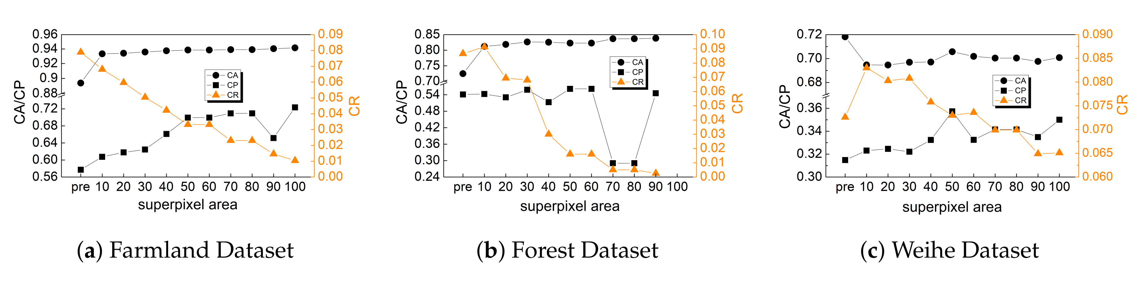
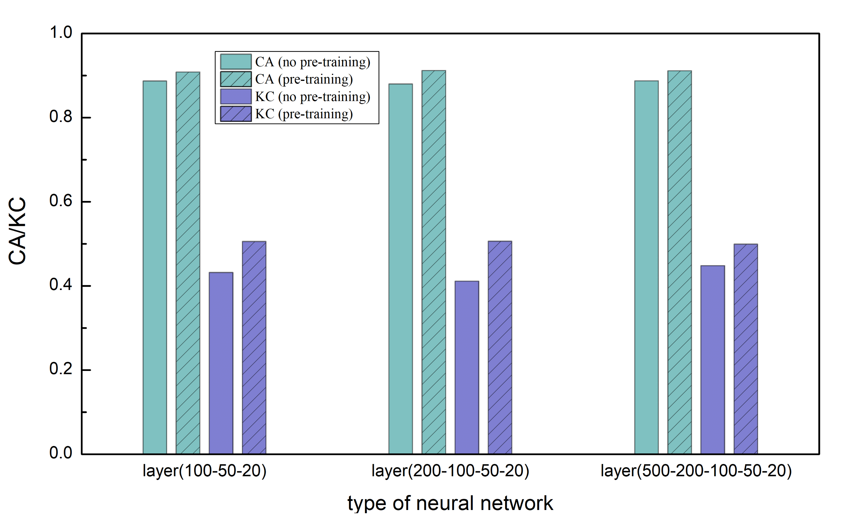
5.3.5. Influence of Pre-Training on Change Detection

For the Farmland Dataset, we conduct comparison experiments on the influence of pre-training on change detection under three types of neural network structures. As shown in Figure 16, the change detection results have a certain improvement in both CA and KC after the neural network is pre-trained. Although unsupervised pre-training plays little role in many supervised learning problems, it is necessary to form a good initialization in this problem. Here, the training set is those obviously changed or unchanged pixel pairs detected in the pre-classification. The test set is the entire remote sensing images, which contain weak changes that are difficult to detect. There could be inconsistent in the distribution of the features of difference between them. After pre-training with broken data, the difference in feature distribution between the training set and the test set would be reduced to a certain extent.

Figure 16. Comparison results of the influence of pre-training on change detection.

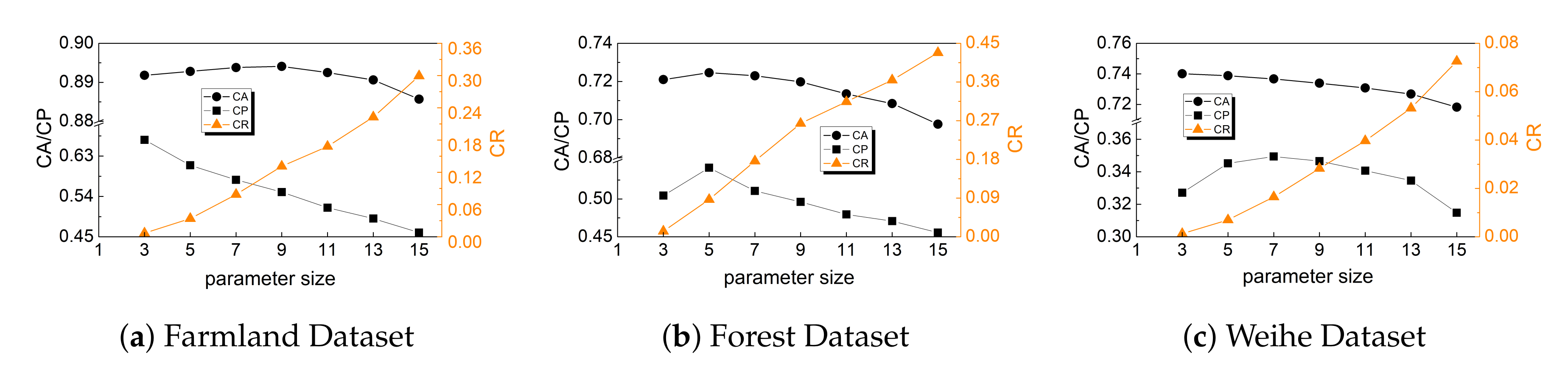
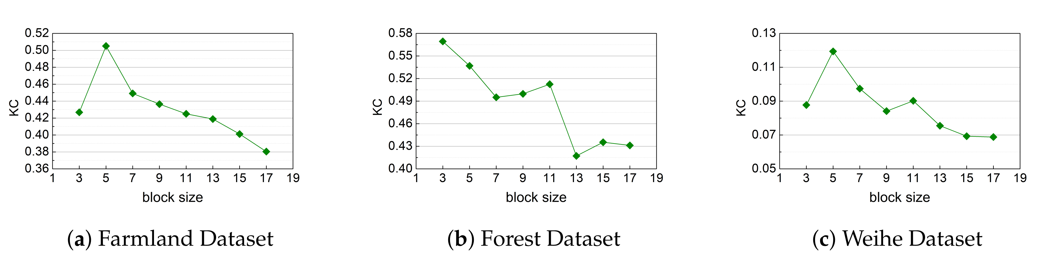
5.3.6. Size of The Pixel Block

In the classification, pixel blocks are utilized as the analysis unit. Here, we employ experiments to explore the effect of pixel block size on the final change detection result. As Figure 17 shows, with the increase in block size, the trends of KC in different datasets are basically consistent. In the Farmland Dataset, KC reaches its peak when block size is 5. Then, KC gradually decreases as block size increases. In the Forest Dataset, KC continues to decrease as block size in the interval (3, 17). Moreover, the changing trend of KC in the Weihe Dataset is basically the same as that in the Farmland Dataset. According to the three datasets, the change detection result is better when the value of block size is 5.

Figure 17. Relationship between parameter size of the pixel block and Kappa Coefficient (KC).

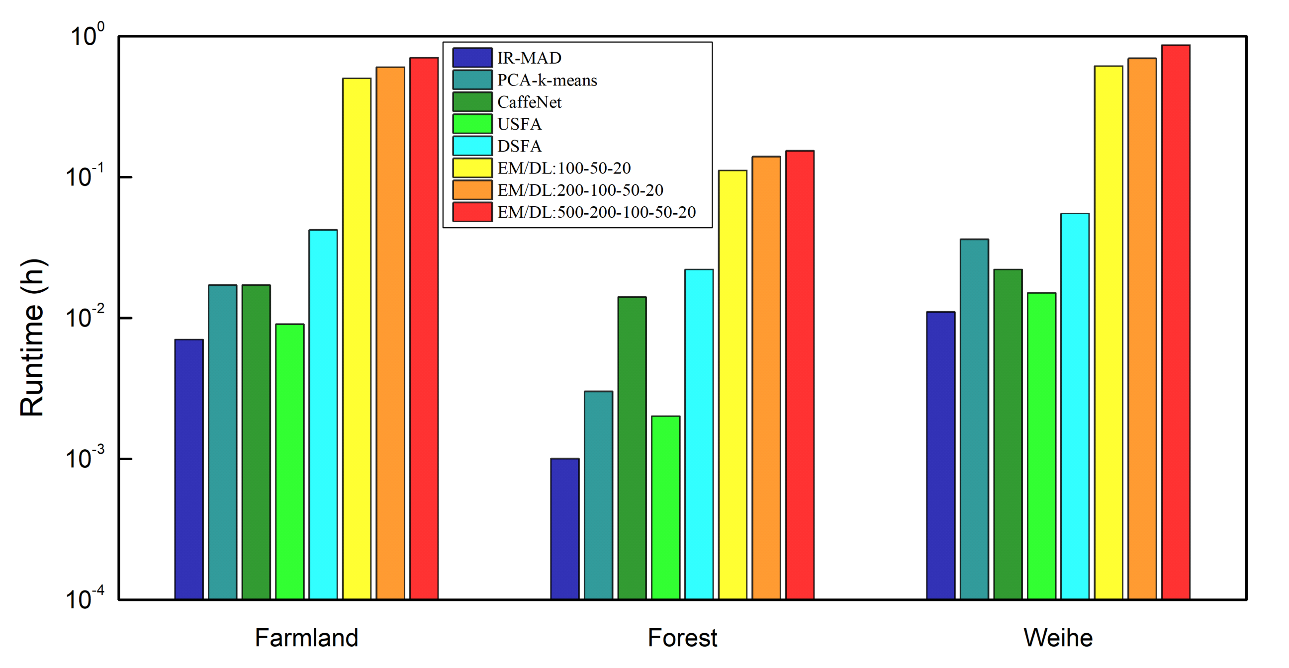
5.4. Runtime Analysis

Here, we analyze the runtime of EM-SDAE and several comparison methods. In our experiments, all methods are implemented in Python and the operating environment is as follows: the type of CPU is Intel(R) Xeon(R) Silver 4110 with a clock rate of 2.10 GHz, and the type of GPU is NVIDIA GEFORCE GTX 1080Ti. As shown in Figure 18, the runtime of IR-MAD, PCA-k-means, CaffeNet, and USFA is lower, and the runtime of DSFA and EM-SDAE is longer because they make use of the neural network. Among all methods, EM-SDAE takes the longest time because the neural network it uses has more parameters. Change detection has certain requirements for time, but the duration is acceptable at the hour level. Although EM-SDAE consumes more runtime, it has higher accuracy. Our method can also be completed in a relatively short time by adjusting some parameters, such as the number of pre-classification iterations, the number of pre-training iterations, and the number of fine-tuning iterations. But the accuracy of the change detection results will decrease a bit.

Figure 18. Comparison of runtime of different methods.

6. Conclusions

Aiming at the change detection of high-resolution remote sensing images, we propose a weakly supervised detection method based on edge mapping and SDAE. It divides the detection procedure into two stages. First, pre-classification is executed by analyzing the difference in the edge maps. Second, a difference extraction network based on SDAE is designed to reduce the noise of remote sensing images and to extract the features of difference from bi-temporal images. For network training, we select reliable samples from pre-classification results. Then, we utilize the neural network to acquire the final change map.

The experimental results of three datasets prove the high efficiency of our method, in which accuracy and KC increase to 91.18% and by 27.19% on average in the first two datasets compared with IR-MAD, PCA-k-means, CaffeNet, USFA, and DSFA. Experiments prove that our method exhibits good performance compared with several existing methods, to a certain degree. However, for some special scenes that require real-time detection, our method cannot complete the detection task in time. In future work, we will further improve the algorithm for real-time detection scenarios.

References

1. Amici, V.; Marcantonio, M.; La Porta, N.; Rocchini, D. A multi-temporal approach in MaxEnt modelling: A new frontier for land use/land cover change detection. Ecol. Inform. 2017, 40, 40–49. [Google Scholar] [CrossRef]
2. Zadbagher, E.; Becek, K.; Berberoglu, S. Modeling land use/land cover change using remote sensing and geographic information systems: Case study of the Seyhan Basin, Turkey. Environ. Monit. Assess. 2018, 190, 494–508. [Google Scholar] [CrossRef] [PubMed]
3. Gargees, R.S.; Scott, G.J. Deep Feature Clustering for Remote Sensing Imagery Land Cover Analysis. IEEE Geosci. Remote Sens. Lett. 2019. [Google Scholar] [CrossRef]
4. Feizizadeh, B.; Blaschke, T.; Tiede, D.; Moghaddam, M.H.R. Evaluating fuzzy operators of an object-based image analysis for detecting landslides and their changes. Geomorphology 2017, 293, 240–254. [Google Scholar] [CrossRef]
5. De Alwis Pitts, D.A.; So, E. Enhanced change detection index for disaster response, recovery assessment and monitoring of accessibility and open spaces (camp sites). Int. J. Appl. Earth Obs. Geoinf. 2017, 57, 49–60. [Google Scholar] [CrossRef]
6. Hao, Y.; Sun, G.; Zhang, A.; Huang, H.; Rong, J.; Ma, P.; Rong, X. 3-D Gabor Convolutional Neural Network for Damage Mapping from Post-earthquake High Resolution Images. In International Conference on Brain Inspired Cognitive Systems; Springer: Berlin/Heidelberg, Germany, 2018; pp. 139–148. [Google Scholar]
7. Gong, M.; Zhao, J.; Liu, J.; Miao, Q.; Jiao, L. Change detection in synthetic aperture radar images based on deep neural networks. IEEE Trans. Neural Networks Learn. Syst. 2015, 27, 125–138. [Google Scholar] [CrossRef]
8. Zhuang, H.; Deng, K.; Fan, H.; Yu, M. Strategies combining spectral angle mapper and change vector analysis to unsupervised change detection in multispectral images. IEEE Geosci. Remote Sens. Lett. 2016, 13, 681–685. [Google Scholar] [CrossRef]
9. Asokan, A.; Anitha, J. Change detection techniques for remote sensing applications: A survey. Earth Sci. Inform. 2019, 12, 143–160. [Google Scholar] [CrossRef]
10. Feng, W.; Sui, H.; Tu, J.; Huang, W.; Xu, C.; Sun, K. A novel change detection approach for multi-temporal high-resolution remote sensing images based on rotation forest and coarse-to-fine uncertainty analyses. Remote Sens. 2018, 10, 1015. [Google Scholar] [CrossRef]
11. Volpi, M.; Tuia, D.; Bovolo, F.; Kanevski, M.; Bruzzone, L. Supervised change detection in VHR images using contextual information and support vector machines. Int. J. Appl. Earth Obs. Geoinf. 2013, 20, 77–85. [Google Scholar] [CrossRef]
12. Mai, D.S.; Ngo, L.T. Semi-supervised fuzzy C-means clustering for change detection from multispectral satellite image. In Proceedings of the 2015 IEEE International Conference on Fuzzy Systems (FUZZ-IEEE), Istanbul, Turkey, 2–5 August 2015; IEEE: Piscataway, NJ, USA, 2015; pp. 1–8. [Google Scholar]
13. Malila, W.A. Change Vector Analysis: An Approach for Detecting Forest Changes with Landsat; Institute of Electrical and Electronics Engineers: West Lafayette, IN, USA, 1980. [Google Scholar]
14. Nielsen, A.A.; Conradsen, K.; Simpson, J.J. Multivariate Alteration Detection (MAD) and MAF Postprocessing in Multispectral, Bitemporal Image Data: New Approaches to Change Detection Studies. Remote Sens. Environ. 1998, 64, 1–19. [Google Scholar] [CrossRef]
15. Celik, T. Unsupervised change detection in satellite images using principal component analysis and k-means clustering. IEEE Geosci. Remote Sens. Lett. 2009, 6, 772–776. [Google Scholar] [CrossRef]
16. Wang, Q.; Yuan, Z.; Du, Q.; Li, X. GETNET: A general end-to-end 2-D CNN framework for hyperspectral image change detection. IEEE Trans. Geosci. Remote Sens. 2018, 57, 3–13. [Google Scholar] [CrossRef]
17. Song, A.; Choi, J.; Han, Y.; Kim, Y. Change Detection in Hyperspectral Images Using Recurrent 3D Fully Convolutional Networks. Remote Sens. 2018, 10, 1827. [Google Scholar] [CrossRef]
18. Xiang, M.; Li, C.; Zhao, Y.; Hu, B. Review on the new technologies to improve the resolution of spatial optical remote sensor. In International Symposium on Advanced Optical Manufacturing and Testing Technologies: Large Mirrors and Telescopes; International Society for Optics and Photonics: San Diego, CA, USA, 2019; Volume 10837, p. 108370C. [Google Scholar]
19. Yu, H.; Yang, W.; Hua, G.; Ru, H.; Huang, P. Change detection using high resolution remote sensing images based on active learning and Markov random fields. Remote Sens. 2017, 9, 1233. [Google Scholar] [CrossRef]
20. Wang, Q.; Zhang, X.; Chen, G.; Dai, F.; Gong, Y.; Zhu, K. Change detection based on Faster R-CNN for high-resolution remote sensing images. Remote Sens. Lett. 2018, 9, 923–932. [Google Scholar] [CrossRef]
21. Lim, K.; Jin, D.; Kim, C.S. Change Detection in High Resolution Satellite Images Using an Ensemble of Convolutional Neural Networks. In Proceedings of the 2018 Asia-Pacific Signal and Information Processing Association Annual Summit and Conference (APSIPA ASC), Honolulu, HI, USA, 12–15 November 2018; IEEE: Piscataway, NJ, USA, 2018; pp. 509–515. [Google Scholar]
22. Xv, J.; Zhang, B.; Guo, H.; Lu, J.; Lin, Y. Combining iterative slow feature analysis and deep feature learning for change detection in high-resolution remote sensing images. J. Appl. Remote Sens. 2019, 13, 024506. [Google Scholar]
23. Tan, K.; Jin, X.; Plaza, A.; Wang, X.; Xiao, L.; Du, P. Automatic change detection in high-resolution remote sensing images by using a multiple classifier system and spectral–spatial features. IEEE J. Sel. Top. Appl. Earth Obs. Remote Sens. 2016, 9, 3439–3451. [Google Scholar] [CrossRef]
24. Cao, G.; Zhou, L.; Li, Y. A new change-detection method in high-resolution remote sensing images based on a conditional random field model. Int. J. Remote Sens. 2016, 37, 1173–1189. [Google Scholar] [CrossRef]
25. El Amin, A.M.; Liu, Q.; Wang, Y. Convolutional neural network features based change detection in satellite images. In First International Workshop on Pattern Recognition; International Society for Optics and Photonics: Tokyo, Japan, 2016; Volume 10011, p. 100110W. [Google Scholar]
26. Du, B.; Ru, L.; Wu, C.; Zhang, L. Unsupervised Deep Slow Feature Analysis for Change Detection in Multi-Temporal Remote Sensing Images. IEEE Trans. Geosci. Remote Sens. 2019, 57, 9976–9992. [Google Scholar] [CrossRef]
27. Nielsen, A.A. The regularized iteratively reweighted MAD method for change detection in multi-and hyperspectral data. IEEE Trans. Image Process. 2007, 16, 463–478. [Google Scholar] [CrossRef] [PubMed]
28. Wu, C.; Du, B.; Zhang, L. Slow Feature Analysis for Change Detection in Multispectral Imagery. IEEE Trans. Geosci. Remote Sens. 2014, 52, 2858–2874. [Google Scholar] [CrossRef]
29. Awrangjeb, M. Effective Generation and Update of a Building Map Database Through Automatic Building Change Detection from LiDAR Point Cloud Data. Remote Sens. 2015, 7, 14119–14150. [Google Scholar] [CrossRef]
30. Guo, J.; Zhou, H.; Zhu, C. Cascaded classification of high resolution remote sensing images using multiple contexts. Inf. Sci. 2013, 221, 84–97. [Google Scholar] [CrossRef]
31. Long, T.; Liang, Z.; Liu, Q. Advanced technology of high-resolution radar: Target detection, tracking, imaging, and recognition. Sci. China Inf. Sci. 2019, 62, 40301. [Google Scholar] [CrossRef]
32. Lv, Z.; Liu, T.; Wan, Y.; Benediktsson, J.A.; Zhang, X. Post-processing approach for refining raw land cover change detection of very high-resolution remote sensing images. Remote Sens. 2018, 10, 472. [Google Scholar] [CrossRef]
33. Guo, Q.; Zhang, J. Change Detection for High Resolution Remote Sensing Image Based on Co-saliency Strategy. In 2019 10th International Workshop on the Analysis of Multitemporal Remote Sensing Images (MultiTemp); IEEE: Piscataway, NJ, USA, 2019; pp. 1–4. [Google Scholar]
34. Saha, S.; Bovolo, F.; Bruzzone, L. Unsupervised Deep Change Vector Analysis for Multiple-Change Detection in VHR Images. IEEE Trans. Geosci. Remote Sens. 2019, 57, 3677–3693. [Google Scholar] [CrossRef]
35. Lv, Z.Y.; Liu, T.F.; Zhang, P.; Benediktsson, J.A.; Lei, T.; Zhang, X. Novel adaptive histogram trend similarity approach for land cover change detection by using bitemporal very-high-resolution remote sensing images. IEEE Trans. Geosci. Remote Sens. 2019, 57, 9554–9574. [Google Scholar] [CrossRef]
36. Peng, D.; Zhang, Y.; Guan, H. End-to-End Change Detection for High Resolution Satellite Images Using Improved UNet++. Remote Sens. 2019, 11, 1382. [Google Scholar] [CrossRef]
37. Hou, B.; Wang, Y.; Liu, Q. A saliency guided semi-supervised building change detection method for high resolution remote sensing images. Sensors 2016, 16, 1377. [Google Scholar] [CrossRef]
38. Zhang, P.; Gong, M.; Su, L.; Liu, J.; Li, Z. Change detection based on deep feature representation and mapping transformation for multi-spatial-resolution remote sensing images. ISPRS J. Photogramm. Remote Sens. 2016, 116, 24–41. [Google Scholar] [CrossRef]
39. Gong, M.; Niu, X.; Zhang, P.; Li, Z. Generative Adversarial Networks for Change Detection in Multispectral Imagery. IEEE Geoence Remote Sens. Lett. 2017, 14, 2310–2314. [Google Scholar] [CrossRef]
40. Lei, Y.; Liu, X.; Shi, J.; Lei, C.; Wang, J. Multiscale superpixel segmentation with deep features for change detection. IEEE Access 2019, 7, 36600–36616. [Google Scholar] [CrossRef]
41. Li, X.; Yuan, Z.; Wang, Q. Unsupervised Deep Noise Modeling for Hyperspectral Image Change Detection. Remote Sens. 2019, 11, 258. [Google Scholar] [CrossRef]
42. Liu, Y.; Cheng, M.M.; Hu, X.; Wang, K.; Bai, X. Richer convolutional features for edge detection. In Proceedings of the IEEE Conference on Computer Vision and Pattern Recognition, Honolulu, HI, USA, 21–26 July 2017; pp. 3000–3009. [Google Scholar]
43. Xie, S.; Tu, Z. Holistically-nested edge detection. In Proceedings of the IEEE International Conference on Computer Vision, Santiago, Chile, 7–13 December 2015; pp. 1395–1403. [Google Scholar]
44. Xu, J.; Jia, Y.; Shi, Z.; Pang, K. An improved anisotropic diffusion filter with semi-adaptive threshold for edge preservation. Signal Process. 2016, 119, 80–91. [Google Scholar] [CrossRef]
45. Achanta, R.; Shaji, A.; Smith, K.; Lucchi, A.; Fua, P.; Süsstrunk, S. SLIC superpixels compared to state-of-the-art superpixel methods. IEEE Trans. Pattern Anal. Mach. Intell. 2012, 34, 2274–2282. [Google Scholar] [CrossRef]
46. Gong, M.; Zhan, T.; Zhang, P.; Miao, Q. Superpixel-based difference representation learning for change detection in multispectral remote sensing images. IEEE Trans. Geosci. Remote Sens. 2017, 55, 2658–2673. [Google Scholar] [CrossRef]
47. Bengio, Y.; Lamblin, P.; Popovici, D.; Larochelle, H. Greedy layer-wise training of deep networks. In Advances in Neural Information Processing Systems; MIT Press: Vancouver, BC, Canada, 2007; pp. 153–160. [Google Scholar]
48. Vincent, P.; Larochelle, H.; Bengio, Y.; Manzagol, P.A. Extracting and composing robust features with denoising autoencoders. In Proceedings of the 25th International Conference on Machine Learning, Helsinki, Finland, 5–9 July 2008; ACM: New York, NY, USA, 2008; pp. 1096–1103. [Google Scholar]
49. Srivastava, N.; Hinton, G.; Krizhevsky, A.; Sutskever, I.; Salakhutdinov, R. Dropout: A simple way to prevent neural networks from overfitting. J. Mach. Learn. Res. 2014, 15, 1929–1958. [Google Scholar]
50. Available online: http://www.rivermap.cn/index.html (accessed on 23 November 2020).
51. Available online: https://www.harrisgeospatial.com/Software-Technology/ENVI/ENVICapabilities/OneButton (accessed on 23 November 2020).
52. Available online: https://github.com/wkentaro/labelme (accessed on 23 November 2020).
Publisher’s Note: MDPI stays neutral with regard to jurisdictional claims in published maps and institutional affiliations.
Article Metrics
Citations
Article Access Statistics
Multiple requests from the same IP address are counted as one view.