Abstract
Recent studies have enhanced the mapping performance of the local climate zone (LCZ), a standard framework for evaluating urban form and function for urban heat island research, through remote sensing (RS) images and deep learning classifiers such as convolutional neural networks (CNNs). The accuracy in the urban-type LCZ (LCZ1-10), however, remains relatively low because RS data cannot provide vertical or horizontal building components in detail. Geographic information system (GIS)-based building datasets can be used as primary sources in LCZ classification, but there is a limit to using them as input data for CNN due to their incompleteness. This study proposes novel methods to classify LCZ using Sentinel 2 images and incomplete building data based on a CNN classifier. We designed three schemes (S1, S2, and a scheme fusion; SF) for mapping 50 m LCZs in two megacities: Berlin and Seoul. S1 used only RS images, and S2 used RS and building components such as area and height (or the number of stories). SF combined two schemes (S1 and S2) based on three conditions, mainly focusing on the confidence level of the CNN classifier. When compared to S1, the overall accuracies for all LCZ classes (OA) and the urban-type LCZ (OAurb) of SF increased by about 4% and 7–9%, respectively, for the two study areas. This study shows that SF can compensate for the imperfections in the building data, which causes misclassifications in S2. The suggested approach can be excellent guidance to produce a high accuracy LCZ map for cities where building databases can be obtained, even if they are incomplete.
1. Introduction
Due to the rapid growth of urbanization since 1950, over 55 percent of the world’s population resides in urban areas, as of 2018 [1]. The migration of the world’s population toward urban areas significantly increases impervious surfaces that absorb solar radiation and reduce convective cooling [2,3]. The stored heat makes the urban areas have a higher temperature than rural surroundings [4,5,6,7], a phenomenon called an urban heat island (UHI). UHI, a leading threat to urban residents, exposing them to higher heat stress and more greenhouse gas emission problems [8], has been analyzed based on various approaches using numerical models or remote sensing (RS) data combined with land cover data, which separate urban areas from their surroundings [9,10]. However, typical land cover products (i.e., moderate resolution imaging spectroradiometer (MODIS) land cover [11] and GlobCover 2009 dataset produced by ESA [12]) have a limited number of classes related to the urban surface. Thus, the different urban structures in various cities are not easily analyzed with the existing land cover products.
To overcome the problem, Stewart and Oke introduced the local climate zone (LCZ), an urban-specified classification system [13]. The LCZ is composed of ten urban-type LCZ classes (LCZ1-10) and seven natural-type classes (LCZA-G; Figure 1). The classification criteria of each class are based on their properties: surface structure (e.g., building height and sky view factor), surface cover (e.g., impervious surface fraction), thermal and radiative characteristics (e.g., surface admittance and albedo), and metabolic information (e.g., anthropogenic heat output) [13]. In particular, the building height is the primary criterion for determining LCZ classes among the ‘high-rise’, ‘mid-rise’, and ‘low-rise’.
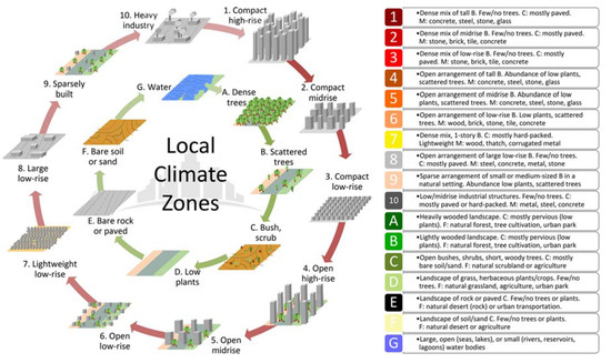
Figure 1.
The local climate zone (LCZ) classes with ‘urban-type’ (LCZ1-10) and ‘natural type’ (LCZA-G) and the characteristics of each class in urban climate research (from Bechtel et al., 2017 after Stewart and Oke, 2012), © CC-BY 4.0.
To obtain the LCZ of a city, there are two primary classification methods: (1) using the geographic information system (GIS) [14,15,16]; and (2) using RS datasets [17,18]. The GIS-based methods collect the building information and geographical features of a study area and then calculate all factors of LCZ classification criteria. Building information is usually obtained from the national geospatial information authorities or OpenStreetMap (OSM) building footprint data [16,19]. Since the GIS-based methods divide LCZ classes based on the physical properties of buildings and urban geography in detail, they often result in high classification accuracy [15,20]. The main disadvantage of the GIS-based methods, however, is that they heavily depend on the accessibility and quality of building and other urban GIS data, which greatly vary between urban areas [20]. Some cities do not have building information as a GIS layer, and some others have building layers but do not update regularly [19]. In Europe, for example, the 10 m resolution rasterized building height layers, called Urban Atlas Building Height 2012 (BH2012), are provided for thirty European cities [21]. Unfortunately, the data coverage is limited within each city boundary excluding data outside the city boundary (i.e., suburban areas). Besides, there are many regions where the BH2012 values are zero even if buildings exist, a critical limitation for classifying LCZ solely from such building height data.
Another widely used method for LCZ classification is using RS imagery based on machine learning algorithms. Bechtel et al. suggested the World Urban Database and Portal Tool (WUDAPT) approach, which is a general LCZ mapping method based on Landsat data and the random forest (RF) classifier [22]. Local experts who have deep background knowledge of each city use high-resolution Google Earth images to extract LCZ reference samples as polygons. These polygons are converted into the raster format for LCZ classification based on RF machine learning. The advantage of WUDAPT is that it uses freely accessible RS datasets, adopts a relatively simple method, and is suitable for the regions where GIS data are unavailable or incomplete [15]. Many kinds of research followed the WUDAPT approach to produce LCZ maps of various world cities [15,23,24,25,26] and shared their reference polygons through the WUDAPT portal (http://www.wudapt.org) [9]. According to the WUDAPT database, while the averaged overall accuracy (OA) of LCZ maps over 90 cities in the world was 74.5% based on the RF method, the averaged OA of only urban LCZ classes in those cities was 59.3%. Therefore, the accuracy of LCZ classification could be further improved, especially for the urban-type LCZ classes, by adopting advanced modeling techniques such as deep learning [18].
Recent studies have applied deep learning approaches to further improve LCZ classification skills using RS data, which bring convolutional neural networks (CNN) into prominence [7,17,27]. Since CNN extracts important spatial features including contextual information from medium-resolution RS imagery, such as Landsat 8 and Sentinel 2, it has proved to be effective in the urban-type LCZ classification [18,27]. In particular, Yoo et al. compared the performances of RF and CNN classifiers for LCZ classification in four mega-cities (Rome, Hong Kong, Madrid, and Chicago) using bitemporal Landsat 8 images [18]. They revealed that CNN showed a 6–8% increase in overall accuracy (OA) compared to WUDAPT workflow (i.e., RF method), while the accuracy for the urban-type classes (OAurb) increased by 10–13% for all four cities. Furthermore, some CNN-based studies used auxiliary data such as urban footprint and OpenStreetMap (OSM) building layers, together with RS data as input variables to improve the LCZ classification accuracy [17]. There are, however, no studies that have used vertical components (i.e., height or number of stories) and horizontal components (i.e., area) of buildings as the main input data of CNN. In fact, it remains very challenging for deep learning to process incomplete information about buildings, which are not spatially seamless unlike RS data.
This present study, therefore, proposes a novel CNN-based LCZ classification approach that can effectively use incomplete building components, along with satellite data, to achieve significant accuracy improvement over two megacities: Berlin, Germany, and Seoul, South Korea. We designed three different schemes: scheme 1 (S1) only uses Sentinel 2 RS data; scheme 2 (S2) uses both RS data and vertical and horizontal building components as input layers to CNN; and scheme 3 (SF) fuses S1 and S2, with proposed assumptions to compensate for the incompleteness of building components. The remaining parts of this paper are organized as follows. Section 2 presents the study area and the data used. Section 3 introduces the methods in detail, including the framework of the three schemes (S1, S2, and SF). In Section 4, the classification accuracy and the LCZ mapping results of the three schemes are compared and discussed. Finally, Section 5 presents the conclusion of this study.
2. Study Area and Data Processing
2.1. Study Area
The study areas are Berlin and Seoul (Figure 2), the capital cities of Germany and South Korea, respectively. Berlin is situated in Northeastern Germany (52.5°N, 13.4°E) with a population of more than 3.7 million inhabitants within an area of 892 km2 in 2019. It has a maritime temperate climate (Cfb) according to the Köppen’s climate classification with an annual mean temperature and precipitation of 9.5 °C and 591 mm, respectively, in 1981–2010 (German Weather Service; the Deutscher Wetterdienst). Berlin is heavily urbanized with about 35% built-up areas and 20% transport and infrastructure areas. In addition, the topography is mainly flat and it has a monocentric urban structure with more compact buildings toward the center of the city.
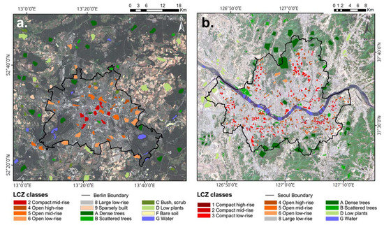
Figure 2.
Study areas of Berlin (a) and Seoul (b) with the local climate zone (LCZ) reference data.
Seoul is located in the northwestern part of South Korea and covers an area of 605 km2. It is one of the most densely populated cities with over 10 million people. The climate of Seoul features a humid continental climate (Dwa) with wet summers and dry winters. According to the Korea Meteorological Administration (KMA), the annual mean temperature and precipitation in Seoul were 12.5 °C and 1450 mm in 1981-2010, respectively, and more than 60% of precipitation is concentrated in summer due to the East Asian monsoon. Urbanization in Seoul has proceeded rapidly since the 1980s, showing an uneven spatial distribution of development. Seoul has a more heterogeneous and complex urban context than Berlin. These two study areas have different climatic characteristics and urban structures, which enables us to evaluate the robustness of the proposed approaches.
2.2. LCZ Reference Data
The LCZ reference polygon data of Berlin were obtained from WUDAPT. For some classes with fewer polygons than ten, additional new reference polygons (i.e., two for LCZ2, six for LCZ4, five for each LCZ5 and 9, and three for LCZC in Berlin) were extracted to make the proposed model more robust. The Berlin LCZs are composed of six urban-type LCZs (LCZ2, 4–6, 8, and 9), and six natural-type LCZs (LCZA-D, F, and G). For Seoul, reference data were sampled manually following the method suggested by Bechtel et al. [22]. Since Seoul has a more compact and heterogeneous urban form than Berlin, we sampled relatively small patches of LCZ classes as reference polygons (Figure 2b). The Seoul LCZs consist of seven urban-type LCZs (LCZ1-6 and 8) and four natural-type LCZs (LCZA, B, D, and G). The LCZ reference polygons were randomly divided into two sets: one for training the model and the other for testing model accuracy. We tried to equally divide the two sets considering both the total number of polygons and the areas they cover for each LCZ class. Even though the recommended minimum area of one LCZ polygon is about 0.125 km2 [13], some LCZ classes have a small number of reference polygons (less than six) that cover areas of only 0.1 km2 (i.e., LCZF for Berlin, and LCZ1 and 6 for Seoul). As some LCZ classes have only a few polygons, it is not desirable to divide them into training and testing sets, often leading to the biased training of the model. Therefore, those classes were labeled ‘red-star’ classes (Table 1), and we extracted the training and testing data within each polygon based on the stratified random sampling approach [18]. Considering the suggested appropriate LCZ mapping scale (30–500 m resolution) and prior research to find the optimal scale [22,28], 50 m was selected as the LCZ mapping scale for the two cities. Finally, all LCZ reference polygons were rasterized to grids with 50 m resolution. The number and area of polygons of the two sets for each LCZ class for the two cities are summarized in Table 1.

Table 1.
Training and test datasets of each LCZ type for Berlin and Seoul. The values in the training and test columns represent the number of polygons. The number of the corresponding pixels (50 m resolution) is shown in parentheses. * is assigned to the red-star classes, which have only a few reference polygons of the LCZ classes. The LCZ figures in the first column are reused from Stewart and Oke [13].
2.3. Satellite Input Data
Sentinel-2A, launched on 23 June 2015, collects data at 13 bands including the visible and near infrared (VNIR) and shortwave infrared (SWIR) with a spatial resolution of 10–60 m. The Sentinel-2A Level-2A (L2A) images for each city were downloaded from Copernicus Open Access Hub (https://scihub.copernicus.eu/). The acquisition dates of the clear-sky Sentinel-2A data are 24 May 2019 for Berlin and 3 May 2019 for Seoul, respectively. Among all bands, VNIR (i.e., bands 2-8) and two SWIR (i.e., bands 11–12) bands were used to classify LCZ, and bands with spatial resolution over 10 m were bilinearly resampled to 10 m in this study.
Landsat 8 Land surface temperature (LST) data, which showed consistent variations within the LCZ classes in the previous studies [24,29], were also used in the present study. Landsat 8 data with 30 m spatial resolution were downloaded from the USGS Earth Explorer (https://earthexplorer.usgs.gov/). LST was retrieved by the single-channel algorithm from atmospherically corrected thermal band 10 using Fast Line-of-sight Atmospheric Analysis of Spectral Hypercubes (FLAASH). A detailed description of retrieving LST can be found in Essa et al. [30]. The one clear-sky LST data for each city were used in this study (i.e., 20 May 2018 for Berlin and 9 May 2018 for Seoul), and they were resampled to 10 m grids using bilinear interpolation.
2.4. Building Data
For Seoul, the building shapefiles are updated every month by the Ministry of Land, Infrastructure and Transport since December 2015. The building shapefiles updated in March 2019 were obtained from the Korea National Spatial Data Infrastructure portal for Seoul (http://data.nsdi.go.kr). For Berlin, the building footprints updated in July 2017 were downloaded from OpenStreetMap (OSM) website (https://www.openstreetmap.org). The building data from OSM could be freely downloaded for non-commercial purposes. After the building areas were calculated using polygons, the building data were rasterized to 10 m resolution for each city (i.e., horizontal layer). In Seoul, the downloaded building shapefiles include the height and the number of stories of each building. Among the two, the number of stories was selected as the vertical layer for Seoul, because the missing rate of building height is higher than that of the number of stories. On the other hand, the building height of Berlin in 2012 was taken from BH2012 with a 10 m spatial resolution (https://land.copernicus.eu). To obtain only the height values of actual buildings, the BH2012 data were extracted using the OSM building shapefile. Note that there is a temporal discrepancy between the building footprints and height information for Berlin.
3. Methodology
3.1. Convolutional Neural Networks (CNN) Classifier
CNN has been widely used in the land cover classification field in recent years [31,32,33,34,35,36]. The advantage of CNN is that it can extract the important spatial features from data without prior knowledge, instead using manually defined spatial features. A typical CNN consists of convolutional layers, pooling layers, and fully connected layer(s) to classify each input image into a single class. In convolutional layers, convolutional filters are optimized to reflect the significant spatial features of the input images. The convolution operation is adopted as a moving window conducting the dot product between the convolutional filters and local regions of the previous layer. Pooling layers return the representative values (i.e., mean or maximum) of the given window. When a k × k pooling layer is adopted, the spatial size of the data is reduced by a factor of k. We used the max-pooling layer, which is widely used in the land cover classification using CNN [18,37,38,39,40]. The pooling layer has some advantages including the invariance to scale difference, the robustness to the noise, and the reduced computational cost [41]. The combination of convolutional and pooling layers is shown as a spatial feature extraction part in Figure 3. Finally, the fully connected layers convert 2-D spatial features into 1-D vectors to conduct the classification as a multilayer perceptron model does. We used the softmax function that converts the output of the last fully connected layer into the probability of each class (equation 1), assigning the output with the maximum probability as the final class.
where is the final result from the output layer for each LCZ class and K is the total number of LCZ classes for each city.
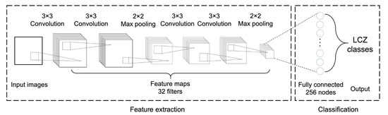
Figure 3.
The structure of the convolutional neural network (CNN) model in this study.
Cross entropy, a widely used loss function that computes the loss between the softmax probability and true label over multiclass classification was adopted in this study (Equation (2)).
where y is the one-hot encoded true label and is the probability vector from the softmax function. The optimization process minimizes the loss of cross entropy finding the best weights of the model by the iterative approach. As the adaptive moment estimation (Adam) is generally used as an optimizer in the classification model due to its faster and stable convergence during the training process [42], we adopted Adam in this study. The nonlinearity of neural networks is from the stacking of nonlinear activation functions. The rectified linear unit (ReLU) is a simple nonlinear function, which returns the identity function at the positive value and zero at the zero or negative value. The simplicity of ReLU can lead it to be more computationally efficient than other activation functions. ReLU also has a faster convergence trend than others, which means that it can achieve a lower loss in fewer iterations [43]. For these reasons, we used the ReLU as an activation function in all convolutional and fully connected layers.
To find the optimal structure and hyperparameters, the heuristic processes are typically used considering both performance and efficiency. After multiple trials changing the structure and hyperparameters (not shown), we used four convolutional layers with 32 filters of 3 × 3 size, two 2 × 2 max-pooling layers after the second and fourth convolutional layers. A fully connected layer with 256 nodes was used after the second max-pooling layer. Finally, the output layer corresponds to the number of LCZ classes. To accelerate the process of both training and classification, an Nvidia GTX 1080Ti graphical process unit (GPU) with 11 GB of memory was used. To train the model, 250 epochs with 256 batch size were taken.
3.2. LCZ Mapping Strategies
We proposed three schemes (S1, S2, and SF) based on CNN with different input variables, to classify LCZ for Berlin and Seoul. Through a multitude of tests, the optimal size of 10 m resolution input features fed into CNN was selected as 55 × 55 for Berlin, and 33 × 33 for Seoul, which cover the focus center LCZ pixel (50 m resolution) and its surrounding area. The reason why the small size of input features is more suitable in Seoul compared to Berlin might be due to the complex and compact urban environment in Seoul. Figure 4 summarizes the process flow of our three proposed schemes.
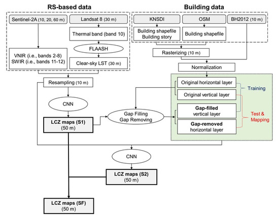
Figure 4.
Schematic diagram of this study showing input variables and processes of each scheme.
Scheme 1 (S1) used 10 m resolution RS images with ten bands (i.e., nine Sentinel reflectances and one Landsat-based LST) as input variables. To reduce the training time, each input image with ten bands was spatially min–max normalized (0–1 range) before being fed into a CNN classifier [18]. After the model training, the 50 m LCZ maps for the two cities were produced by S1.
Scheme 2 (S2) used two building components—such as horizontal (area) and vertical (height or number of stories) layers—as the input variables, together with those of S1. There were, however, regions in which the building footprints exist but the height (or the number of stories) values were missing (Table 2).
Table 2.
Missing rates of height values in the entire study area and in urban-type LCZ reference data.
To deal with these imperfect vertical building components in the training process, we implemented the following procedure. First, the 50 m LCZ map produced in S1 was resampled to 10 m. Based on the 10 m LCZ map, the mean building heights (or the number of stories) of each LCZ class were calculated from the vertical layer. In this step, only buildings with height information (Berlin) or the number of stories (Seoul) larger than 0 were used for the average. Next, we defined the vertical value–missing regions, in which height or the number of stories values were zero (or none), even if buildings are located in the 10 m resolution vertical layer. The vertical value–missing regions were filled with the calculated mean height or number of stories of the assigned LCZ class, based on the S1 map. These simulated layers were called gap-filled vertical layers. A gap-removed horizontal layer was also produced in cases where the vertical value was missing, and so the area value was also removed.
The S2 was trained using the gap-filled vertical layer as the vertical component and the original area layer as a horizontal component. For the testing and mapping processes, the original vertical layer was used as a vertical component, and the gap-removed horizontal layer was used as the horizontal component, to identify the effect of building imperfections in the model. All building layers were also min–max normalized as the range of 0–1, except the missing (or zero) value. To be distinguished from the actual building value, the missing regions were assigned as −0.01, which is outside the 0–1 range. The input variables for S1 and S2 are summarized in Table 3.
Table 3.
The input variables for S1 and S2.
In S2, two different types of data-processing—gap-filling and gap-removing—were adopted for training and testing datasets to use the horizontal and vertical components of the building data. Since the gap-filled vertical layers could be virtual (not actual data), the gap-removal processing was applied for test datasets to exclude the contamination of imperfect building data. Thus, for the vertical value–missing regions, both horizontal and vertical information was deleted as if there were no buildings there. There were also some regions in which the building footprints (i.e., shapefiles) were not recorded in the first place, so neither horizontal nor vertical information was available. Over those regions, CNN could be confused when satellite datasets detected the existence of building based on the spectral characteristics of the land surface, but additional building layers have missing values (i.e., −0.01). Thus, the mismatch between satellite images and ancillary building data could lead to the confusion of CNN, making it hard to discriminate LCZ classes with a high confidence level in S2. To solve this shortcoming, we developed a new scheme—the fusion of outputs from S1 and S2—and named it scheme fusion (SF).
At first, the maximum values of softmax probability calculated for the final LCZ class assignment were calculated per pixel in S1 and S2 LCZ maps, and then defined as follows:
SF was predominantly based on the outputs from S2, but it was substituted with the outputs from S1 with the following conditions:
- Condition 1: PS1 > PS2.
- Condition 2: If S1 is classified as urban-type LCZ (LCZ1-10), but S2 is classified as natural-type (LCZA-G).
- Condition 3: If S1 is classified as compact urban-type LCZ (LCZ1-3) and PS1 is 1 (100% confident), but S2 is not (LCZ4-G).
Condition 1 was based on the softmax probability, which connoted the confidence of each model [34]. If PS2 is lower than PS1, it may be doubtful whether the addition of building data confused CNN for LCZ classification. Condition 2 was based on the high quality of CNN classifier’s ability to distinguish urban and natural-types, already verified in Yoo et al. [18]. Thus, S1 and S2 may yield the same results on the question of whether urban (LCZ1-10) or not (LCZA-G). If, however, S1 and S2 show different results as urban-type in S1 and natural-type in S2, then we should be cautious about the possibility of misclassification in S2 because of the incomplete building information. Condition 3 concentrated on the possibility of misclassification due to the partial removal or omission of building information. If S1 classified a specific region as ‘compact’ (LCZ1-3) with its PS1 as 1 (100%) but S2 classified there as another class (LCZ4-G), we should consider whether the result of S2 is wrong. Since the classified result with PS1 as 1 is such a reliable result, if it changed to another class in S2, we need to suspect that adding incomplete building information disrupted the CNN decisions. Therefore, pixels of the S2 LCZ map, which fulfilled at least one of the above three conditions, were replaced with the results of S1.
3.3. Modeling and Accuracy Assessment
Among training samples (i.e., training set), a randomly selected 10% of samples were used to optimize the weights and biases in the CNN model. In this step in S1 and S2, the best parameters were selected based on the overall accuracy (OA; Equation (3)) among 250 epochs. After the three schemes were constructed (S1, S2, and SF), the separated test sets were evaluated. For an accuracy assessment, three metrics were calculated: first the OA, then the overall accuracy of the LCZ classes only to urban-types (OAurb; Equation (4)), and the overall accuracy of the urban versus natural LCZ types (OAu; Equation (5)). They were calculated as follows:
where is the number of pixels classified as the ith LCZ class and is the number of pixels correctly classified as the ith LCZ class, and are the number of ground truths of all classes and only built-up classes, respectively, and k and m are the total numbers of LCZ classes and total built-up classes. In addition, we evaluated the F1-score (Equation (6)), which is a harmonic mean value of the producer’s accuracy (PA) and user’s accuracy (UA) for each LCZ class to identify the classification performance by class. The F1-score is a widely used matrix for LCZ modeling assessment because it represents how similar the PA and UA are [18,28].
3.4. Evaluation for the Regions of Missing Building Information
To identify each model’s capability to deal with the missing building information, we compared the performance of the three schemes (S1, S2, and SF) using simulated test sets and the removal of building information. In other words, the regions where vertical and horizontal components exist in the original test sets were randomly replaced by non-building values (i.e., −0.01) at six different removal rates (0%, 20%, 40%, 60%, 80%, and 100%). Then, the accuracy of the simulated test sets was compared by using the trained models of S1, S2, and SF.
4. Results and Discussion
4.1. Overall Accuracy Assessment
Table 4 shows the accuracy assessment results of S1, S2, and SF for Berlin and Seoul. S2 of Seoul increased 3% in OA and 8% in OAurb compared to S1. The increase in the accuracy was much larger than that of Qiu et al. [17], who reported that using OSM binary building data together with Sentinel reflectance in residual CNN (ResNet) did not improve LCZ classification accuracy significantly (only 1% increase in weighted accuracy) compared to that only using Sentinel datasets. Using the quantitative building components (i.e., area and height) rather than the simple binary information (i.e., building or not) is likely the reason for the greater accuracy for Seoul S2. It should be noted that S2 of Berlin showed a slight increase in OA (1%), a slight decrease in OAurb (1.1%), but a significant decrease in OAu (7%), when compared to S1 (Table 4). The opposite performance of S2 between Berlin and Seoul might be caused by the different missing rate of building components used in S2 between Seoul and Berlin. The missing rate of vertical values differed by city and LCZ classes (Table 2). Since the height information of Berlin was only available within the city boundary, Berlin had higher missing rates of height especially 100% for LCZ9 and 41% for LCZ8 that have many pixels beyond the boundary. This kind of incompleteness might increase the possibility of misclassification when the building components were added. Based on the S1 and S2 results for both cities, whether building information benefits LCZ classification is dependent on the quality of the building data. If perfect building data (100% accurate) were added, we would expect a significant increase in LCZ classification accuracy, especially for urban-type LCZs. However, if building information is incomplete, there might be a chance to decrease the accuracy of LCZ classification.
Table 4.
Accuracy assessment results for S1, S2, and SF of Berlin and Seoul. The highest values of three accuracy metrics (OA, OAurb, and OAu) are written in bold.
The proposed SF showed the highest values for all accuracy metrics (i.e., OA, OAurb, and OAu) for Berlin and Seoul (Table 4). In particular, SF of Berlin showed a significant increase of 7% in OAurb from its S1 OAurb, while S2 showed a slight increase in OAurb. Moreover, the drop in OAu for S2 was recovered by 98.2% in SF of Berlin and 99.6% in SF of Seoul. This implies that the proposed fusion method can compensate for the misclassifications of S2, caused by missing values in building information, by selectively choosing the better results between S1 and S2 based on the three conditions. These accuracies of SF are significantly better than those from the WUDAPT method (OA of 68% and OAurb of 76% for Berlin and OA of 93% and OAurb of 64% for Seoul). In addition, the OA of SF in Berlin is comparable with that from Rosentreter et al. (OA of 87.7%) [27], although each map used a slightly different study coverage and had a different sampling technique.
Figure 5 and Figure 6 show the F1-scores of each LCZ class and the confusion matrices of S1, S2, and SF, respectively. Some LCZ classification studies based on CNN using RS data (almost the same as with S1) have reported the limitations of those methods resulting in confusion within the height standard (i.e., LCZ1-3 or LCZ4-6) or density standard (i.e., between LCZ1&4 or LCZ2&5 or LCZ3&6) [18,27]. It should be noted that S2 showed a significant increase in F1-scores for urban-type LCZ classes for both cities when compared to those of S1 (Figure 5). For Berlin, S2 improved the LCZ classification, especially reducing the confusion between LCZ5 and other urban-type LCZ, and reduced misclassification of LCZ6 to LCZ5 or LCZ9, which often occurred in S1 (Figure 6). For Seoul, all urban-type LCZ classes were better discriminated in S2 than in S1. Fonte et al. reported that only using binary OSM data combined with the WUDAPT method did not increase the classification accuracy much within the urban-type LCZ [44]. To overcome this, S2 added building information, such as height, to help discriminate LCZ classes from each other within urban types, while S1 revealed the difficulties in discriminating them.
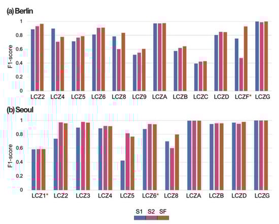
Figure 5.
F1-scores of each LCZ class for the three schemes (S1, S2, and SF) in Berlin (a) and Seoul (b). The asterisk (*) indicates the red-star classes.
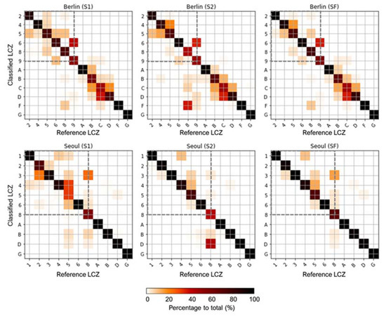
Figure 6.
Confusion matrices of three schemes for Berlin and Seoul. The most accurate model results are presented by percentages to the total numbers of ground reference data. The dashed box indicates the urban-type LCZ classes.
All classes of Seoul, except LCZ8, had higher F1-scores for S2 than S1, while S2 of Berlin showed a decrease in F1-scores in some classes when compared to S1 (Figure 5). For Berlin, LCZ4 and LCZ8 showed higher F1-scores in S1 than in S2. S2 of Berlin and Seoul misclassified LCZ8 as natural-type LCZs, LCZF, and LCZD, respectively (Figure 6). These misclassifications of urban-type LCZ to the nature types might be attributed to high missing rates of building data, 100% for LCZ9 in Berlin, 41% for LCZ8 in Berlin, and 54% for LCZ8 in Seoul (Table 2). All reference samples of LCZ9 in Berlin had empty building height layers and all missing values were filled with no building data (i.e., −0.01). This might lead to the misclassification from LCZ9 to the natural-type LCZB or LCZF. The incomplete building information could have caused the misclassifications of urban-type LCZs to the natural-type LCZs and decreased the classification accuracy of S2, especially in OAu.
It is not surprising that adding building information had little effect on improving classification performance in natural-type LCZs. Natural-type LCZs of Seoul consistently showed high F1-scores in all schemes, while F1-scores of Berlin for such LCZ classes were not as high as Seoul, but quite stable in all schemes as Seoul except for LCZF (Figure 5). Some urban-type LCZs that were misclassified as natural-type LCZs in S2 caused the decrease in F1-scores of natural-type LCZs. For example, the misclassification from LCZ8 to LCZF in S2 of Berlin resulted in a decrease in F1-scores of LCZF. Similarly, the confusion from LCZ8 to LCZD in S2 of Seoul caused a decrease in F1-scores of LCZD. Except for these misclassifications due to incomplete building components as mentioned above, there were minor differences between S1 and S2 about natural-type LCZs in both cities.
It should be noted that the classes that showed low F1-scores in S2 achieved high F1-scores when SF was applied. The misclassifications of urban-type LCZs to natural-type LCZs found in S2 were reduced in SF and confusion within urban-type LCZs in S1 was also improved in SF (Figure 6). Moreover, both cities had the highest F1-scores in SF for most LCZ classes when compared to S1 and S2. This implies that the three conditions proposed in SF accurately detected the misclassifications caused by incomplete building data and improved classification within urban-type LCZs. However, LCZ4 of Berlin showed the highest score in S1, and LCZ5 of Seoul showed the highest score in S2 (Figure 5). This implies that the three conditions of SF did not always guarantee the highest F1-score for every class. The F1-scores of the red-star classes need to be carefully interpreted in Figure 6. For example, there was no F1-score difference between the schemes for LCZ1 in Seoul. This might be due to the positive bias in the test results as the test sets were randomly divided with training sets within one polygon [18,28].
4.2. Mapping LCZ for Three Schemes
Figure 7 and Figure 8 show the 50 m resolution LCZ maps of Berlin and Seoul using the three schemes—S1, S2, and SF. In the first subset (Box 1) of Berlin and that of Seoul, where the vertical layer of each city had almost no missing values, S2 showed better classification results than S1 (Figure 7). Compared to the Google Earth images, the region packed with many mid-rise buildings in Berlin was well classified as LCZ2 in S2 while some of them were misclassified as LCZ8 in S1 (Figure 9a). For Seoul, S2 well divided the distinct boundary between mid-rise and high-rise apartments (Figure 9b). This implies that adding horizontal and vertical building information might better detect the boundary of building complexes and correctly distinguish classes with different heights, such as LCZ4 and LCZ5, which is difficult to do using only RS images.
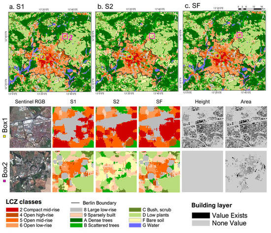
Figure 7.
LCZ maps with the best classification models of three schemes (S1, S2, and SF) for Berlin. Building height and area layers from BH2012 and OSM are also included. The enlarged results of each scheme and building components for two subset areas (Box 1 and Box 2) are presented. Box 1 was full of building information, while Box 2 had many missing values in building information.
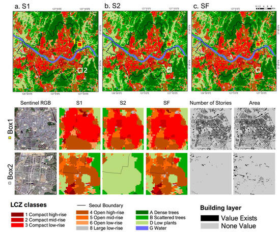
Figure 8.
LCZ maps with the best classification models of three schemes (S1, S2, and SF) for Seoul. Building story and area layers from KNSDI are also present. The enlarged results of each scheme and building components for two subset areas (Box 1 and Box 2) are presented. Box 1 was full of building information, while Box 2 had many missing values in building information.
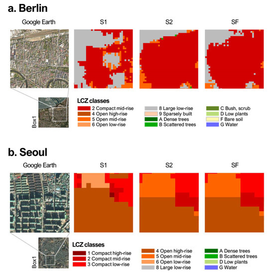
Figure 9.
Detailed comparison of S1, S2, and SF in the first subset domain (Box 1) in Figure 8 for Berlin (a) and Seoul (b). Google Earth images of each region are also presented.
However, in the second subset (Box 2) of Berlin and Seoul, S2 did not improve the accuracy of urban-type LCZ classification. The Box 2 of Berlin was surrounded by farmland (not shown), and the mid-rise and low-rise buildings were located in the center of the box. S1 classified well with LCZ5, LCZ6, and LC9, while S2 confused this area with LCZF (Figure 7). In Box 2 of Seoul, high-rise and mid-rise housing complexes were well detected with LCZ4 and LCZ5, respectively, in S1, but none of them were correctly detected in S2 (Figure 8). The common characteristic of these two subsets was the empty vertical layers. Buildings in these subsets were misclassified as natural-type LCZ classes, such as bare soil or low plants, in S2. This implies that S2 did not always produce better classification results than S1 in either city, especially where building data were incomplete.
The LCZ maps of SF for Berlin and Seoul showed the best performance by improving the accuracy of urban-type LCZ classes based on building data and the three conditions to improve the misclassifications caused by the missing building data (Figure 7 and Figure 8). For the subsets that had empty vertical layers (i.e., Box 2), the LCZ map of SF was almost the same as that of S1. For the subsets that had complete vertical layers, the map of SF seemed a mixture of S1 and S2 in Berlin (Box 1; Figure 7), while it was almost the same as the map of S2 in Seoul (Box 1; Figure 8). One possible reason is that S2 of Berlin and Seoul were trained using building data with different missing rates. In the case of Berlin, many missing values in the vertical layer were gap-filled and used for model training. With these imperfect building components, S2 of Berlin classified some urban-type LCZs with lower confidence levels than S1. According to the first and third conditions of SF, the results of S2 with low PS2 values may have been substituted by the results of S1 with high PS1 values in the first subset of Berlin (Box 1; Figure 7). Seoul had fewer missing values than Berlin so that S2 of Seoul might have been able to classify urban-type LCZ classes with high PS2 values then these results were maintained in SF.
Table 5 shows the ratio of each LCZ class area to the total area on the maps of S1, S2, and SF. Compared to S1, the percentage of urban-type LCZ classes (LCZ1-10) in both Berlin and Seoul increased by about 1% in SF. Within the urban-type LCZ of Berlin, the ratio of LCZ5 decreased by about 1.3% in SF compared to S1, and LCZ6 increased by about 1.2%. In S1, LCZ6 and other urban-type LCZs were often confused with LCZ5 (Figure 6). LCZ5 (open mid-rise) and LCZ6 (Open low-rise) might be well classified in SF based on the building height data. For Seoul, the ratio of LCZ3 and LCZ5 in SF increased by about 1–2% compared to S1. This might be because LCZ3 (compact low-rise) was confused with LCZ2 (Compact mid-rise), and LCZ5 was misclassified into several other LCZ classes (i.e., LCZ4) in S1. On the other hand, LCZ3 and LCZ5 were generally well classified in SF (Figure 6). Moreover, in S2, the ratios of some natural-type LCZs in both cities (LCZB and F for Berlin and LCZB and D for Seoul) were significantly higher than those of S1 and SF (Table 5). One possible reason is due to the misclassification of urban-type to natural-type LCZs caused by incomplete building information. The problem has been improved in SF, resulting in the ratios for the natural-type LCZs similar to S1.
Table 5.
The area ratio of each LCZ class to the total area on the maps of S1, S2, and SF for both Berlin and Seoul.
4.3. Impact of Missing Building Information
Figure 10 shows the accuracy assessment results when removing building components in the test data at different rates (0%, 20%, 40%, 60%, 80%, and 100%). S1 showed the constant results in all OA indices because S1 used only RS images so that the removals of building data did not affect the results of S1. When compared to S1, OA, OAurb, and OAu of S2 decreased with the increasing removal rate for both cities. The decline of OAurb for the two cities was similar from 0 to 40% removal rates. However, with the removal rate >40%, OAurb sharply decreased for Seoul compared to the OAurb of Berlin (Figure 10c,d). For the compact and complex urban environments found in Seoul, the building components could highly affect mapping accuracy on LCZ classification. For relatively mid-density cities like Berlin, on the other hand, the RS-based input data seems to complement the incomplete building data relatively well. Interestingly, the OAurb and OAu sharply decreased when all buildings were removed, when compared to the lower removal rates (i.e., 80% removal). One possible reason is that, if there is minimal building information, the region could be classified as at least an urban-type LCZ, but if building information is completely omitted, the region has a high possibility of being classified as a natural-type LCZ. In addition, it is not surprising that the accuracy of S2 significantly decreased with the increasing removal building rate for compact urban-type LCZ (LCZ2 for Berlin and LCZ1-3 for Seoul), compared to other LCZ classes based on the F1-score (Figure S1). It should be noted that the OA, OAurb, and OAu of SF were higher or comparable to those of S1, even when the removal rate increased to 100% for two cities. In our suggested SF methodology, regions with missing building information are easily distinguishable from the natural areas that actually have no buildings.
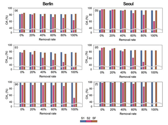
Figure 10.
Accuracy assessment results (OA (a,b), OAurb (c,d) and OAu (e,f)) of three schemes with removing building components at different rates (0%, 20%, 40%, 60%, 80%, and 100%) for Berlin (a,c,e) and Seoul (b,d,f).
4.4. Novelty, Limitations, and Future Directions
To our knowledge, this is the first study conducted to improve LCZ classification accuracy based on building information (area and height) and satellite data through a CNN-based classification approach. While some studies have used building data, such as OSM, as an input variable of CNN or canonical correlation forest (CCF) models [17,45], they did not use the quantitative characteristics of buildings, such as height. In particular, this study proposed a novel method that uses the classification confidence of CNN to search for regions of incomplete building data. The positive effect of the inclusion of building characteristics was shown by the significant improvement in LCZ classification accuracy.
One limitation of the proposed method is the difficulty of transferring this model from one city to another. The sources of the building data are different for each city. Moreover, each city has different standards for height (or the number of stories) that distinguish high-rise from low-rise buildings due to unique urban environments [21]. However, until recently, many studies produced an LCZ map for each city based on the WUDAPT workflow [46,47,48]. Therefore, if building data are available for these cities, a more accurate LCZ map could be produced for each city, based on the suggested method of this study.
The three conditions used for our proposed scheme fusion also have limitations. Although the two cities in this study (Berlin and Seoul) were selected to show the general use of this method, the incomplete building data could not be fully filtered by the three conditions. However, there have been several recent attempts to fill the data gaps. Urban footprint extraction techniques have been proposed based on deep learning models [49,50]. In addition, some studies have attempted to estimate building height using a synthetic aperture radar (SAR) [51,52,53]. By utilizing these methods, more complete and accurate building characteristic data could be used for CNN to produce higher quality LCZ maps.
Recently, research has been conducted to extract building height using medium-resolution SAR images on a continental scale [51,52], but the spatial resolution (i.e., 0.5–2 km) and accuracy are not yet sufficiently fine for LCZ mapping. In the future when the open-access global urban footprint data or high-resolution building height extracted from free RS images data are provided, our suggested method will be an excellent option to produce a higher accuracy global LCZ map.
5. Conclusions
This study proposed a novel method to combine the RS data and building information to improve CNN-based LCZ classification accuracy. Three schemes (i.e., S1, S2, and SF) were constructed for Berlin and Seoul. S1 used only RS data, S2 used RS data and building data together, and SF fused S1 and S2 to compensate for incomplete building data. Compared to S1, SF increased accuracy by about 3–4% in OA and about 7–9% in OAurb for both cities. This study revealed that adding building data improved urban-type LCZ classification accuracy by providing horizontal and vertical information about buildings. This study also showed that the incompleteness of building data caused misclassifications that could be compensated by SF. Some pixels of SF, however, still showed misclassified results, because they could not be perfectly filtered by the suggested three conditions. More precise conditions for scheme fusion need to be tested to develop more accurate LCZ maps in the future. This study provided the first comprehensive assessment of classification performance when building datasets were added as input variables for a CNN-based approach. When high-resolution urban footprint and height data are provided on a global scale, this suggested method will give directions on using building components to produce a global LCZ map with high accuracy in a deep learning-based approach.
Supplementary Materials
The following are available online at https://www.mdpi.com/2072-4292/12/21/3552/s1, Figure S1. The variation of F1-scores of three schemes with removing building components at different rates (20%, 40%, 60%, 80%, and 100%)
Author Contributions
Conceptualization, C.Y.; formal analysis, C.Y. and Y.L.; investigation, C.Y. and Y.L.; methodology, C.Y., Y.L., D.C., and J.I.; supervision, J.I.; validation, C.Y. and Y.L.; writing—original draft, C.Y., Y.L., D.C., and D.H.; writing—review and editing, J.I. All authors have read and agreed to the published version of the manuscript.
Funding
This research was supported by the Korea Meteorological Administration Research and Development Program under Grant KMIPA 2017–7010, by the Korea Environment Industry & Technology Institute (KEITI) through its Urban Ecological Health Promotion Technology Development Project funded by the Korea Ministry of Environment (MOE) (2020002770001), by the Institute for Information & communications Technology Promotion (IITP) supported by the Ministry of Science and ICT (MSIT), Korea (IITP-2020-2018-0-01424), and by the support of ´R&D Program for Forest Science Technology (Project No. FTIS 2020179A00-2022-BB01) provided by Korea Forest Service (Korea Forestry Promotion Institute). CY was also supported by Global PhD Fellowship Program through the National Research Foundation of Korea (NRF), funded by the Ministry of Education (NRF-2018H1A2A1062207).
Acknowledgments
We would like to thank WUDAPT (the World Urban Database and Access Portal Tools project, www.wudapt.org), and all the contributors for LCZ ground-truth samples, in particular Je-Woo Hong.
Conflicts of Interest
The authors declare no conflict of interest.
References
- DESA, U. World Urbanization Prospects 2018: Highlights; ST/ESA/SER. A/421; Department of Economic and Social Affairs Population Division: New York, NY, USA, 2019. [Google Scholar]
- Mohan, M.; Sati, A.P.; Bhati, S. Urban sprawl during five decadal period over National Capital Region of India: Impact on urban heat island and thermal comfort. Urban Clim. 2020, 33, 100647. [Google Scholar] [CrossRef]
- Weng, Q.; Lu, D.; Schubring, J. Estimation of land surface temperature–vegetation abundance relationship for urban heat island studies. Remote Sens. Environ. 2004, 89, 467–483. [Google Scholar] [CrossRef]
- Argüeso, D.; Evans, J.P.; Fita, L.; Bormann, K.J. Temperature response to future urbanization and climate change. Clim. Dyn. 2014, 42, 2183–2199. [Google Scholar] [CrossRef]
- Oleson, K.; Monaghan, A.; Wilhelmi, O.; Barlage, M.; Brunsell, N.; Feddema, J.; Hu, L.; Steinhoff, D. Interactions between urbanization, heat stress, and climate change. Clim. Chang. 2015, 129, 525–541. [Google Scholar] [CrossRef]
- Shahmohamadi, P.; Che-Ani, A.; Maulud, K.; Tawil, N.; Abdullah, N. The impact of anthropogenic heat on formation of urban heat island and energy consumption balance. Urban Stud. Res. 2011. [Google Scholar] [CrossRef]
- Yoo, C.; Im, J.; Park, S.; Quackenbush, L.J. Estimation of daily maximum and minimum air temperatures in urban landscapes using MODIS time series satellite data. ISPRS J. Photogramm. Remote Sens. 2018, 137, 149–162. [Google Scholar] [CrossRef]
- Chapman, S.; Watson, J.E.; Salazar, A.; Thatcher, M.; McAlpine, C.A. The impact of urbanization and climate change on urban temperatures: A systematic review. Landsc. Ecol. 2017, 32, 1921–1935. [Google Scholar] [CrossRef]
- Bechtel, B.; Demuzere, M.; Mills, G.; Zhan, W.; Sismanidis, P.; Small, C.; Voogt, J. SUHI analysis using Local Climate Zones—A comparison of 50 cities. Urban Clim. 2019, 28, 100451. [Google Scholar] [CrossRef]
- Umezaki, A.S.; Ribeiro, F.N.D.; de Oliveira, A.P.; Soares, J.; de Miranda, R.M. Numerical characterization of spatial and temporal evolution of summer urban heat island intensity in São Paulo, Brazil. Urban Clim. 2020, 32, 100615. [Google Scholar] [CrossRef]
- Friedl, M.A.; Sulla-Menashe, D.; Tan, B.; Schneider, A.; Ramankutty, N.; Sibley, A.; Huang, X. MODIS Collection 5 global land cover: Algorithm refinements and characterization of new datasets. Remote. Sens. Environ. 2010, 114, 168–182. [Google Scholar] [CrossRef]
- Bontemps, S.; Defourny, P.; Van Bogaert, E.; Arino, O.; Kalogirou, V.; Perez, J.R. GLOBCOVER 2009 Products Description and Validation Report. 2011. Available online: http://ionia1.esrin.esa.int/docs/GLOBCOVER2009_Validation_Report_2 (accessed on 1 August 2020).
- Stewart, I.D.; Oke, T.R. Local climate zones for urban temperature studies. Bull. Am. Meteorol. Soc. 2012, 93, 1879–1900. [Google Scholar] [CrossRef]
- Unger, J.; Lelovics, E.; Gál, T. Local Climate Zone mapping using GIS methods in Szeged. Hung. Geogr. Bull. 2014, 63, 29–41. [Google Scholar] [CrossRef]
- Wang, R.; Ren, C.; Xu, Y.; Lau, K.K.-L.; Shi, Y. Mapping the local climate zones of urban areas by GIS-based and WUDAPT methods: A case study of Hong Kong. Urban Clim. 2018, 24, 567–576. [Google Scholar] [CrossRef]
- Zheng, Y.; Ren, C.; Xu, Y.; Wang, R.; Ho, J.; Lau, K.; Ng, E. GIS-based mapping of Local Climate Zone in the high-density city of Hong Kong. Urban Clim. 2018, 24, 419–448. [Google Scholar] [CrossRef]
- Qiu, C.; Schmitt, M.; Mou, L.; Ghamisi, P.; Zhu, X.X. Feature importance analysis for local climate zone classification using a residual convolutional neural network with multi-source datasets. Remote Sens. 2018, 10, 1572. [Google Scholar] [CrossRef]
- Yoo, C.; Han, D.; Im, J.; Bechtel, B. Comparison between convolutional neural networks and random forest for local climate zone classification in mega urban areas using Landsat images. ISPRS J. Photogramm. Remote Sens. 2019, 157, 155–170. [Google Scholar] [CrossRef]
- Fan, H.; Zipf, A.; Fu, Q.; Neis, P. Quality assessment for building footprints data on OpenStreetMap. Int. J. Geogr. Inf. Sci. 2014, 28, 700–719. [Google Scholar] [CrossRef]
- Geletič, J.; Lehnert, M.; Dobrovolný, P. Land surface temperature differences within local climate zones, based on two central European cities. Remote Sens. 2016, 8, 788. [Google Scholar] [CrossRef]
- Demuzere, M.; Bechtel, B.; Middel, A.; Mills, G. Mapping Europe into local climate zones. PLoS ONE 2019, 14, e0214474. [Google Scholar] [CrossRef]
- Bechtel, B.; Alexander, P.J.; Böhner, J.; Ching, J.; Conrad, O.; Feddema, J.; Mills, G.; See, L.; Stewart, I. Mapping local climate zones for a worldwide database of the form and function of cities. ISPRS Int. J. Geo-Inf. 2015, 4, 199–219. [Google Scholar] [CrossRef]
- Beck, C.; Straub, A.; Breitner, S.; Cyrys, J.; Philipp, A.; Rathmann, J.; Schneider, A.; Wolf, K.; Jacobeit, J. Air temperature characteristics of local climate zones in the Augsburg urban area (Bavaria, southern Germany) under varying synoptic conditions. Urban Clim. 2018, 25, 152–166. [Google Scholar] [CrossRef]
- Cai, M.; Ren, C.; Xu, Y.; Lau, K.K.-L.; Wang, R. Investigating the relationship between local climate zone and land surface temperature using an improved WUDAPT methodology–A case study of Yangtze River Delta, China. Urban Clim. 2018, 24, 485–502. [Google Scholar] [CrossRef]
- Giridharan, R.; Emmanuel, R. The impact of urban compactness, comfort strategies and energy consumption on tropical urban heat island intensity: A review. Sustain. Cities Soc. 2018, 40, 677–687. [Google Scholar] [CrossRef]
- Kaloustian, N.; Bechtel, B. Local climatic zoning and urban heat island in Beirut. Procedia Eng. 2016, 169, 216–223. [Google Scholar] [CrossRef]
- Rosentreter, J.; Hagensieker, R.; Waske, B. Towards large-scale mapping of local climate zones using multitemporal Sentinel 2 data and convolutional neural networks. Remote Sens. Environ. 2020, 237, 111472. [Google Scholar] [CrossRef]
- Verdonck, M.-L.; Okujeni, A.; van der Linden, S.; Demuzere, M.; De Wulf, R.; Van Coillie, F. Influence of neighbourhood information on ‘Local Climate Zone’mapping in heterogeneous cities. Int. J. Appl. Earth Obs. Geoinf. 2017, 62, 102–113. [Google Scholar] [CrossRef]
- Geletič, J.; Lehnert, M.; Savić, S.; Milošević, D. Inter-/intra-zonal seasonal variability of the surface urban heat island based on local climate zones in three central European cities. Build. Environ. 2019, 156, 21–32. [Google Scholar] [CrossRef]
- Essa, W.; van der Kwast, J.; Verbeiren, B.; Batelaan, O. Downscaling of thermal images over urban areas using the land surface temperature–impervious percentage relationship. Int. J. Appl. Earth Obs. Geoinf. 2013, 23, 95–108. [Google Scholar] [CrossRef]
- Kim, M.; Lee, J.; Im, J. Deep learning-based monitoring of overshooting cloud tops from geostationary satellite data. GIScience Remote Sens. 2018, 55, 763–792. [Google Scholar] [CrossRef]
- Liu, T.; Abd-Elrahman, A.; Morton, J.; Wilhelm, V.L. Comparing fully convolutional networks, random forest, support vector machine, and patch-based deep convolutional neural networks for object-based wetland mapping using images from small unmanned aircraft system. GIScience Remote Sens. 2018, 55, 243–264. [Google Scholar] [CrossRef]
- Sothe, C.; De Almeida, C.; Schimalski, M.; La Rosa, L.; Castro, J.; Feitosa, R.; Dalponte, M.; Lima, C.; Liesenberg, V.; Miyoshi, G. Comparative performance of convolutional neural network, weighted and conventional support vector machine and random forest for classifying tree species using hyperspectral and photogrammetric data. GIScience Remote Sens. 2020, 57, 369–394. [Google Scholar] [CrossRef]
- Zhang, C.; Pan, X.; Li, H.; Gardiner, A.; Sargent, I.; Hare, J.; Atkinson, P.M. A hybrid MLP-CNN classifier for very fine resolution remotely sensed image classification. ISPRS J. Photogramm. Remote Sens. 2018, 140, 133–144. [Google Scholar] [CrossRef]
- Zhao, S.; Liu, X.; Ding, C.; Liu, S.; Wu, C.; Wu, L. Mapping rice paddies in complex landscapes with convolutional neural networks and phenological metrics. GIScience Remote Sens. 2020, 57, 37–48. [Google Scholar] [CrossRef]
- Yu, X.; Wu, X.; Luo, C.; Ren, P. Deep learning in remote sensing scene classification: A data augmentation enhanced convolutional neural network framework. GIScience Remote Sens. 2017, 54, 741–758. [Google Scholar] [CrossRef]
- Al-Najjar, H.A.; Kalantar, B.; Pradhan, B.; Saeidi, V.; Halin, A.A.; Ueda, N.; Mansor, S. Land cover classification from fused DSM and UAV images using convolutional neural networks. Remote Sens. 2019, 11, 1461. [Google Scholar] [CrossRef]
- Fu, G.; Liu, C.; Zhou, R.; Sun, T.; Zhang, Q. Classification for high resolution remote sensing imagery using a fully convolutional network. Remote Sens. 2017, 9, 498. [Google Scholar] [CrossRef]
- Lee, J.; Han, D.; Shin, M.; Im, J.; Lee, J.; Quackenbush, L.J. Different Spectral Domain Transformation for Land Cover Classification Using Convolutional Neural Networks with Multi-Temporal Satellite Imagery. Remote Sens. 2020, 12, 1097. [Google Scholar] [CrossRef]
- Marcos, D.; Volpi, M.; Kellenberger, B.; Tuia, D. Land cover mapping at very high resolution with rotation equivariant CNNs: Towards small yet accurate models. ISPRS J. Photogramm. Remote Sens. 2018, 145, 96–107. [Google Scholar] [CrossRef]
- Boureau, Y.-L.; Ponce, J.; LeCun, Y. A theoretical analysis of feature pooling in visual recognition. In Proceedings of the 27th international conference on machine learning (ICML-10), Haifa, Israel, 21–24 June 2010; pp. 111–118. [Google Scholar]
- Kingma, D.P.; Ba, J. Adam: A method for stochastic optimization. In Proceedings of the International Conference on Learning Representations, San Diego, CA, USA, 7–9 May 2015. [Google Scholar]
- Krizhevsky, A.; Sutskever, I.; Hinton, G.E. Imagenet classification with deep convolutional neural networks. In Proceedings of the Advances in Neural Information Processing Systems, Lake Tahoe, NV, USA, 3–6 December 2012; pp. 1097–1105. [Google Scholar]
- Fonte, C.C.; Lopes, P.; See, L.; Bechtel, B. Using OpenStreetMap (OSM) to enhance the classification of local climate zones in the framework of WUDAPT. Urban Clim. 2019, 28, 100456. [Google Scholar] [CrossRef]
- Zhang, G.; Ghamisi, P.; Zhu, X.X. Fusion of heterogeneous earth observation data for the classification of local climate zones. IEEE Trans. Geosci. Remote Sens. 2019, 57, 7623–7642. [Google Scholar] [CrossRef]
- Brousse, O.; Wouters, H.; Demuzere, M.; Thiery, W.; Van de Walle, J.; Van Lipzig, N.P. The local climate impact of an African city during clear-sky conditions—Implications of the recent urbanization in Kampala (Uganda). Int. J. Climatol. 2020. [Google Scholar] [CrossRef]
- Mu, Q.; Miao, S.; Wang, Y.; Li, Y.; He, X.; Yan, C. Evaluation of employing local climate zone classification for mesoscale modelling over Beijing metropolitan area. Meteorol. Atmos. Phys. 2020, 132, 315–326. [Google Scholar] [CrossRef]
- Ochola, E.M.; Fakharizadehshirazi, E.; Adimo, A.O.; Mukundi, J.B.; Wesonga, J.M.; Sodoudi, S. Inter-local climate zone differentiation of land surface temperatures for Management of Urban Heat in Nairobi City, Kenya. Urban Clim. 2020, 31, 100540. [Google Scholar] [CrossRef]
- Aung, H.T.; Pha, S.H.; Takeuchi, W. Building footprint extraction in Yangon city from monocular optical satellite image using deep learning. Geocarto Int. 2020, 1–21. [Google Scholar] [CrossRef]
- Milosavljević, A. Automated Processing of Remote Sensing Imagery Using Deep Semantic Segmentation: A Building Footprint Extraction Case. ISPRS Int. J. Geo-Inf. 2020, 9, 486. [Google Scholar] [CrossRef]
- Li, M.; Koks, E.; Taubenböck, H.; van Vliet, J. Continental-scale mapping and analysis of 3D building structure. Remote Sens. Environ. 2020, 245, 111859. [Google Scholar] [CrossRef]
- Li, X.; Zhou, Y.; Gong, P.; Seto, K.C.; Clinton, N. Developing a method to estimate building height from Sentinel-1 data. Remote Sens. Environ. 2020, 240, 111705. [Google Scholar] [CrossRef]
- Soergel, U.; Michaelsen, E.; Thiele, A.; Cadario, E.; Thoennessen, U. Stereo analysis of high-resolution SAR images for building height estimation in cases of orthogonal aspect directions. ISPRS J. Photogramm. Remote Sens. 2009, 64, 490–500. [Google Scholar] [CrossRef]


Publisher’s Note: MDPI stays neutral with regard to jurisdictional claims in published maps and institutional affiliations. |
© 2020 by the authors. Licensee MDPI, Basel, Switzerland. This article is an open access article distributed under the terms and conditions of the Creative Commons Attribution (CC BY) license (http://creativecommons.org/licenses/by/4.0/).