An Analytical Framework for Accurate Traffic Flow Parameter Calculation from UAV Aerial Videos


Abstract
1. Introduction
Related Works
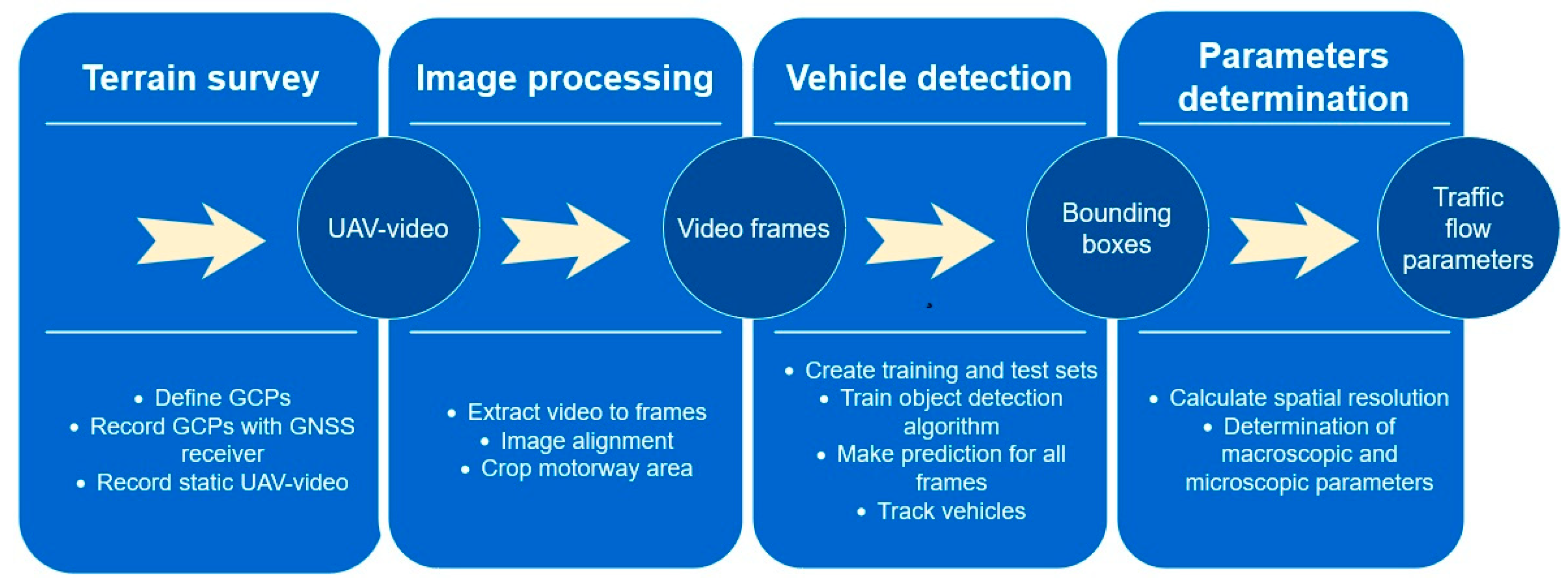
2. Data Collections and Methods
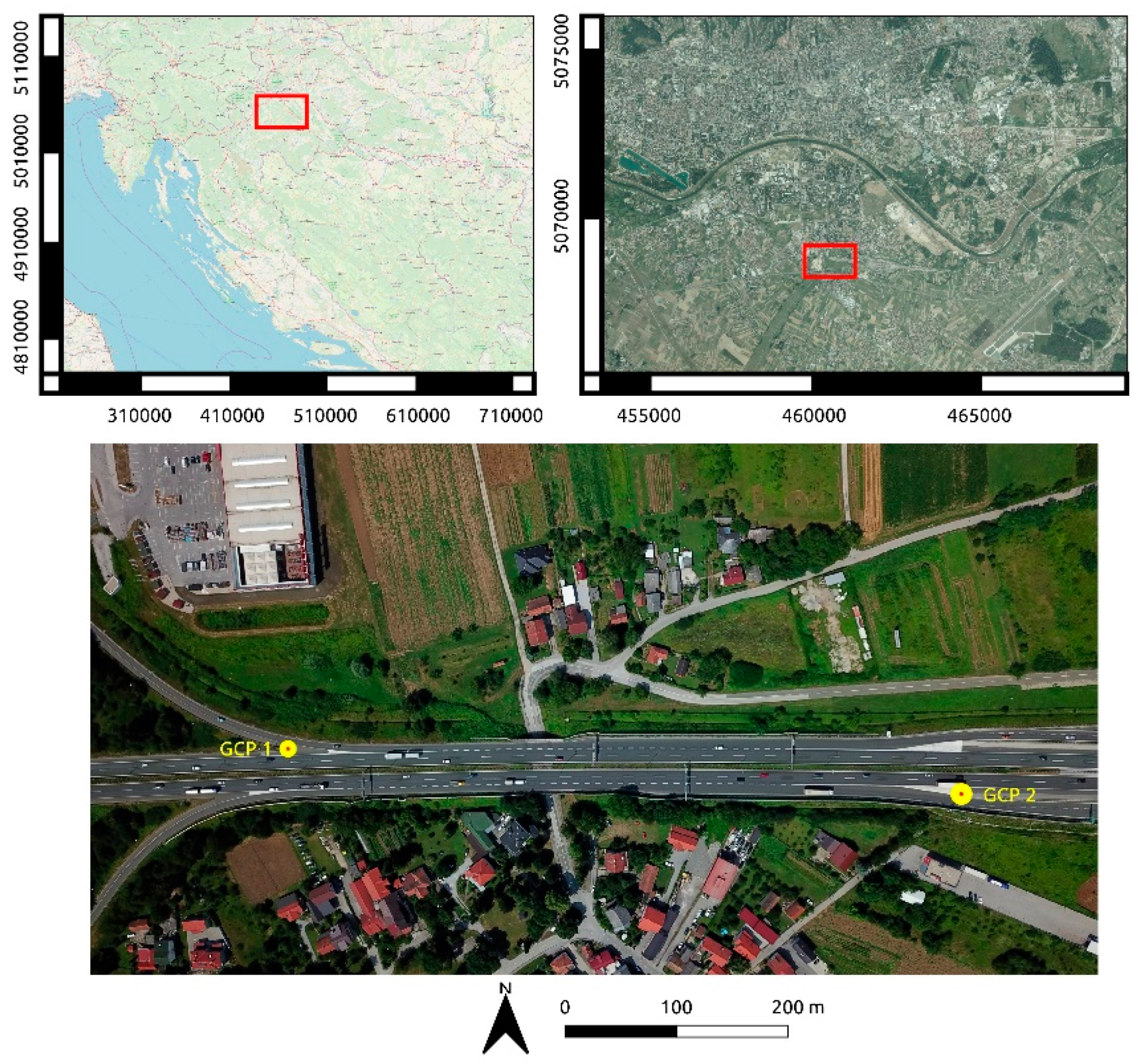
2.1. Terrain Survey
2.2. Image Processing
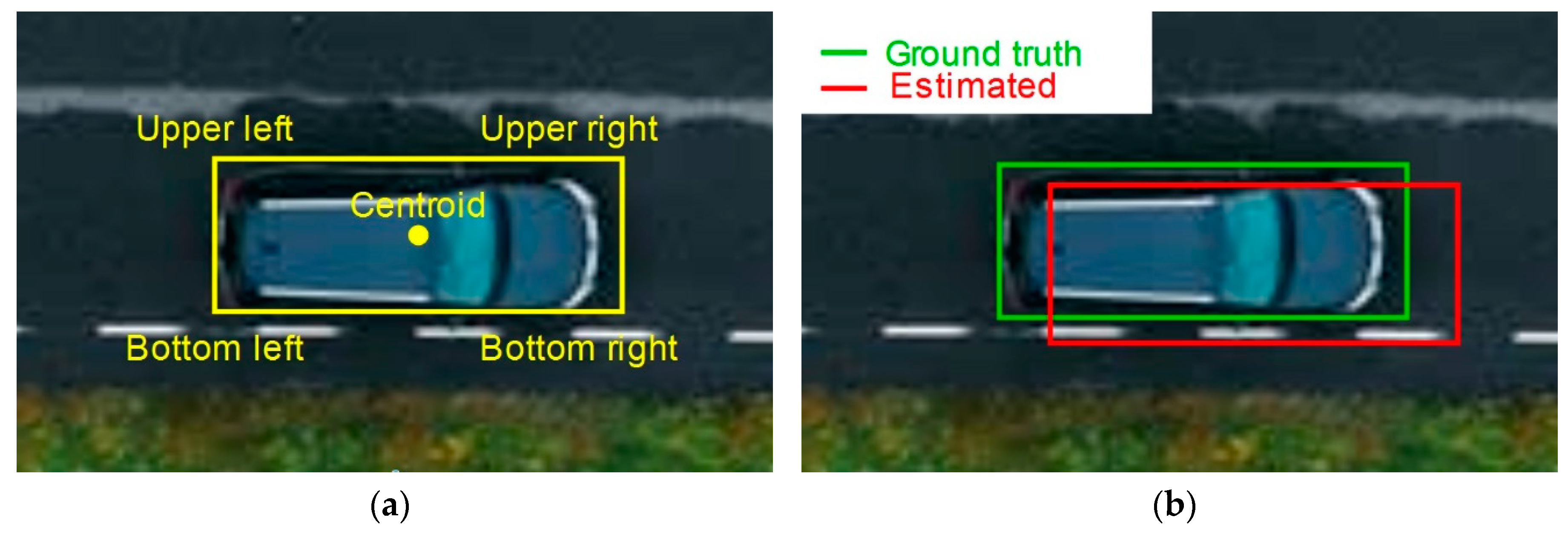
2.3. Vehicle Detection
2.4. Parameters Determination
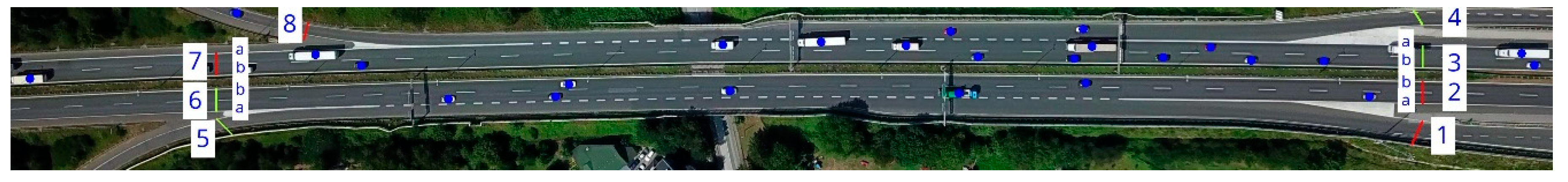
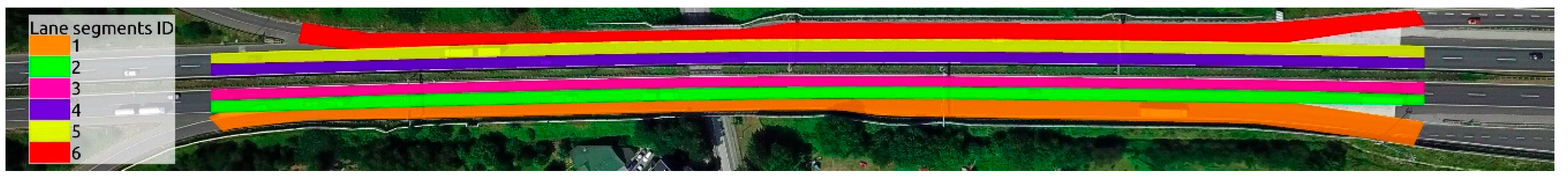
2.4.1. Macroscopic Traffic Flow Parameters
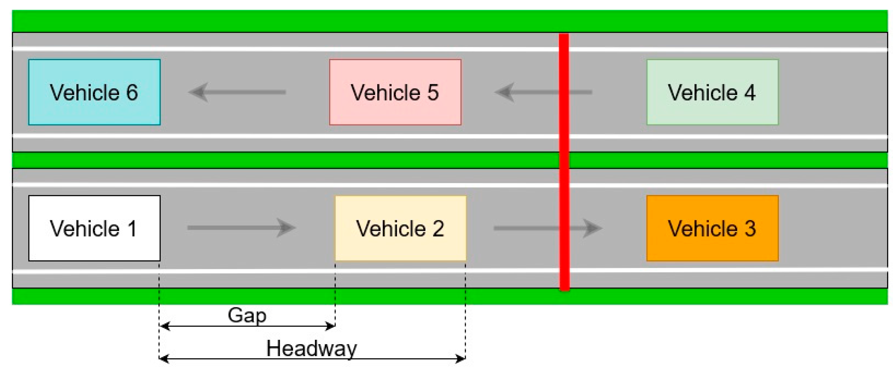
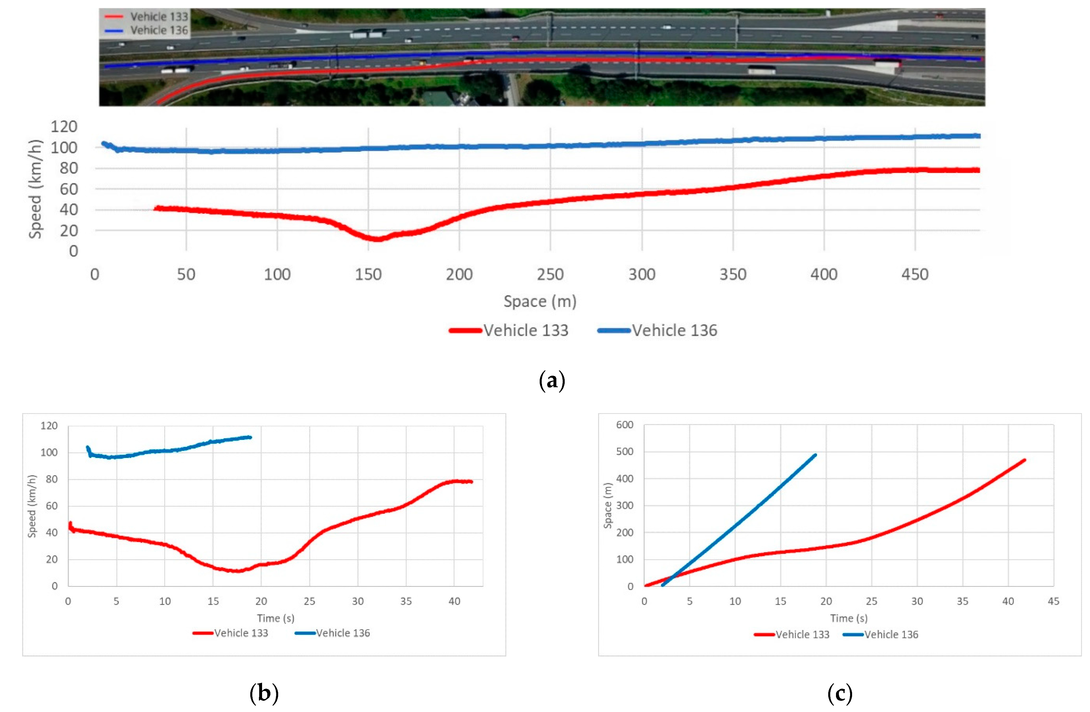
2.4.2. Microscopic Traffic Flow Parameters
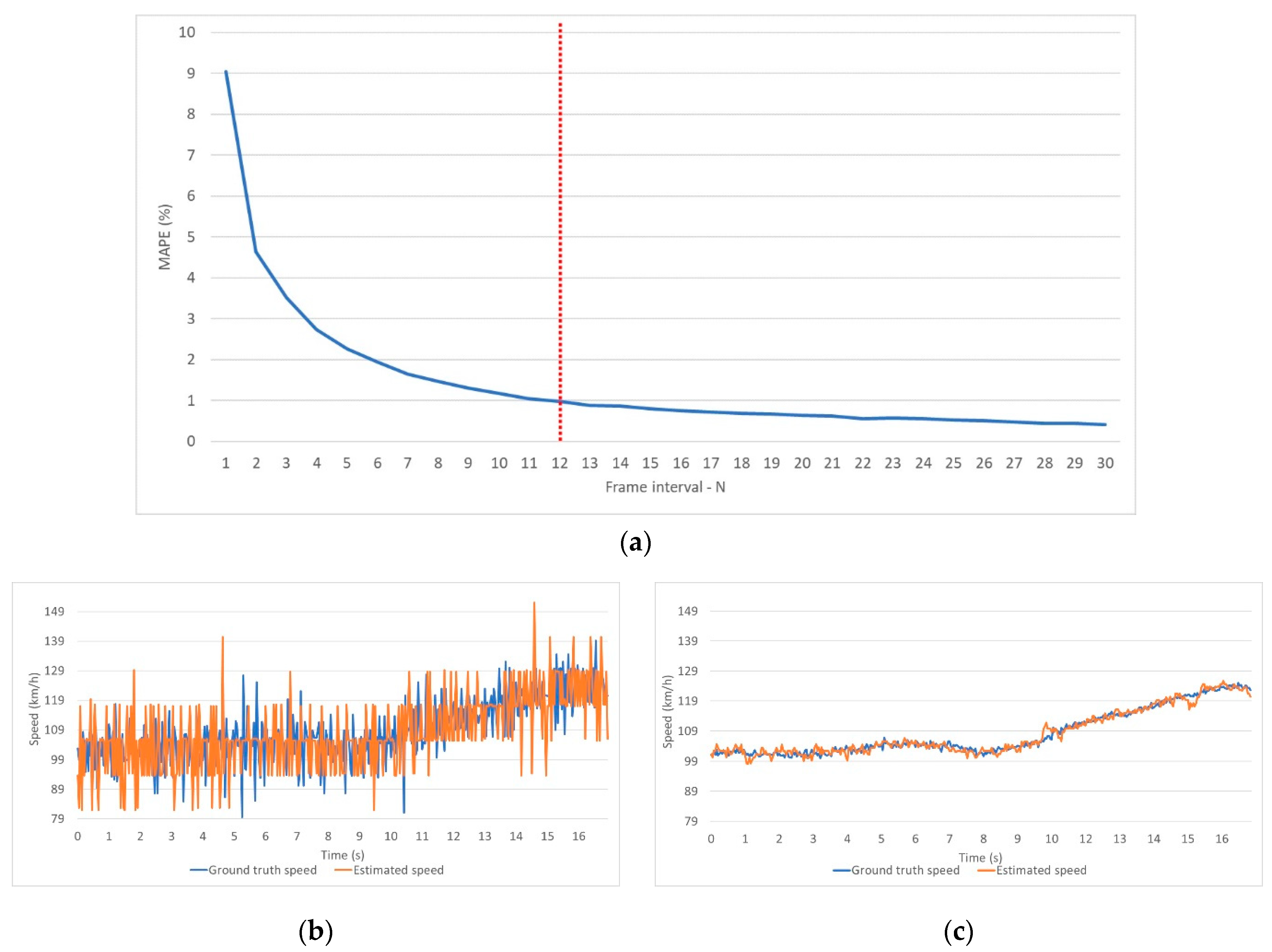
3. Results
4. Discussion
5. Conclusions
Author Contributions
Funding
Conflicts of Interest
References
- European Automobile Manufacturers Association Vehicles in use Europe 2019. 2019. Available online: https://www.acea.be/uploads/statistic_documents/ACEA_Report_Vehicles_in_use-Europe_2017.pdf (accessed on 10 March 2020).
- Mathew, T.V.; Rao, K.V.K. Fundamental parameters of traffic flow. In Introduction to Transportation Engineering; National Program on Technical Education and Learning (NPTEL): Mumbay, India, 2007; pp. 1–8. [Google Scholar]
- Hoogendoorn, S.; Knoop, V. Traffic flow theory and modelling. Transp. Syst. Transp. Policy Introd. 2012, 125–159. [Google Scholar]
- Leduc, G. Road Traffic Data: Collection Methods and Applications; JRC: Seville, Spain, 2008. [Google Scholar]
- Handscombe, J.; Yu, H.Q. Low-Cost and Data Anonymised City Traffic Flow Data Collection to Support Intelligent Traffic System. Sensors 2019, 19, 347. [Google Scholar] [CrossRef] [PubMed]
- Martinez, A.P. Freight Traffic data in the City of Eindhoven; University of Technology Eindhoven: Eindhoven, The Netherlands, 2015. [Google Scholar]
- Kanistras, K.; Martins, G.; Rutherford, M.J.; Valavanis, K.P. A survey of unmanned aerial vehicles (UAVs) for traffic monitoring. In Proceedings of the 2013 International Conference on Unmanned Aircraft Systems (ICUAS), Atlanta, GA, USA, 28–31 May 2013; pp. 221–234. [Google Scholar]
- SESAR Joint Undertaking European Drones Outlook Study. SESAR 2016. Available online: http://www.sesarju.eu/sites/default/files/documents/reports/European_Drones_Outlook_Study_2016.pdf (accessed on 12 March 2020).
- El-Sayed, H.; Chaqfa, M.; Zeadally, S.; Puthal, A.D. A Traffic-Aware Approach for Enabling Unmanned Aerial Vehicles ( UAVs ) in Smart City Scenarios. IEEE Access 2019, 7, 86297–86305. [Google Scholar] [CrossRef]
- Menouar, H.; Guvenc, I.; Akkaya, K.; Uluagac, A.S.; Kadri, A.; Tuncer, A. UAV-Enabled Intelligent Transportation Systems for the Smart City: Applications and Challenges. IEEE Commun. Mag. 2017, 55, 22–28. [Google Scholar] [CrossRef]
- Ghazzai, H.; Menouar, H.; Kadri, A. On the Placement of UAV Docking Stations for Future Intelligent Transportation Systems. In Proceedings of the 2017 IEEE 85th Vehicular Technology Conference (VTC Spring), Sydney, Australia, 4–7 June 2017; pp. 1–6. [Google Scholar]
- Beg, A.; Qureshi, A.R.; Sheltami, T.; Yasar, A. UAV-enabled intelligent traffic policing and emergency response handling system for the smart city. Pers. Ubiquitous Comput. 2020, 1–18. [Google Scholar] [CrossRef]
- Khan, M.A.; Ectors, W.; Bellemans, T.; Janssens, D.; Wets, G. Unmanned Aerial Vehicle-Based Traffic Analysis: A Case Study for Shockwave Identification and Flow Parameters Estimation at Signalized Intersections. Remote Sens. 2018, 10, 458. [Google Scholar] [CrossRef]
- Ke, R.; Li, Z.; Tang, J.; Pan, Z.; Wang, Y. Real-Time Traffic Flow Parameter Estimation From UAV Video Based on Ensemble Classifier and Optical Flow. IEEE Trans. Intell. Transp. Syst. 2019, 20, 54–64. [Google Scholar] [CrossRef]
- Chen, X.; Li, Z.; Yang, Y.; Qi, L.; Ke, R. High-Resolution Vehicle Trajectory Extraction and Denoising From Aerial Videos. IEEE Trans. Intell. Transp. Syst. 2020, 1–13. [Google Scholar] [CrossRef]
- Fedorov, A.; Nikolskaia, K.; Ivanov, S.; Shepelev, V.; Minbaleev, A. Traffic flow estimation with data from a video surveillance camera. J. Big Data 2019, 6. [Google Scholar] [CrossRef]
- Wang, L.; Chen, F.; Yin, H. Detecting and tracking vehicles in traffic by unmanned aerial vehicles. Autom. Constr. 2016, 72, 294–308. [Google Scholar] [CrossRef]
- Transport Development Strategy of the Republic of Croatia (2017–2030)—Development of Sectoral Transport Strategies; Ministry of the Sea, Transport and Infrastructure: Zagreb, Croatia, 2013; ISBN 9788578110796.
- Transportation Research Board. Highway Capacity Manual 6th Edition: A Guide for Multimodal Mobility Analysis; The National Academies Press: Washington, DC, USA, 2016. [Google Scholar] [CrossRef]
- Awad, A.I.; Hassaballah, M. (Eds.) Studies in Computational Intelligence; Springer International Publishing: Cham, Switzerland, 2016; Volume 630, ISBN 978-3-319-28852-9. [Google Scholar]
- Pieropan, A.; Björkman, M.; Bergström, N.; Kragic, D. Feature Descriptors for Tracking by Detection: A Benchmark. arXiv 2016, arXiv:1607.06178. [Google Scholar]
- Aglave, P.; Kolkure, V.S. Implementation of High Performance Feature Extraction Method Using Oriented Fast and Rotated Brief Algorithm. Int. J. Res. Eng. Technol. 2015, 4, 394–397. [Google Scholar] [CrossRef]
- Zhou, Q.; Li, X. STN-Homography: Estimate homography parameters directly. arXiv 2019, arXiv:1906.02539. [Google Scholar]
- Chum, O.; Matas, J.; Kittler, J. Locally optimized RANSAC. In Proceedings of the Joint Pattern Recognition Symposium; Springer: Berlin/Heidelberg, Germany, 2003; Volume 2781, pp. 236–243. [Google Scholar]
- Fischler, M.A.; Bolles, R.C. Random Sample Consensus: A Paradigm for Model Fitting with Applications to Image Analysis and Automated Cartography; Morgan Kaufmann Publishers, Inc.: Burlington, MA, USA, 1987. [Google Scholar]
- Ma, Y.; Soatto, S.; Košecká, J.; Sastry, S.S. Reconstruction from Two Uncalibrated Views. In An Invitation to 3-D Vision; Springer: Berlin/Heidelberg, Germany, 2004; pp. 171–227. [Google Scholar]
- Yague-Martinez, N.; De Zan, F.; Prats-Iraola, P. Coregistration of Interferometric Stacks of Sentinel-1 TOPS Data. IEEE Geosci. Remote Sens. Lett. 2017, 14, 1002–1006. [Google Scholar] [CrossRef]
- Zhao, Z.-Q.; Zheng, P.; Xu, S.-T.; Wu, X. Object Detection With Deep Learning: A Review. IEEE Trans. Neural Netw.Learn. Syst. 2019, 30, 3212–3232. [Google Scholar] [CrossRef] [PubMed]
- JJiao, L.; Zhang, F.; Liu, F.; Yang, S.; Li, L.; Feng, Z.; Qu, R. A Survey of Deep Learning-Based Object Detection. IEEE Access 2019, 7, 128837–128868. [Google Scholar] [CrossRef]
- Li, B.; Liu, Y.; Wang, X. Gradient Harmonized Single-Stage Detector. Proc Conf AAAI Artif Intell 2019, 33, 8577–8584. [Google Scholar] [CrossRef]
- Sun, B.; Xu, Y.; Li, C.; Yu, J. Analysis of the Impact of Google Maps’ Level on Object Detection. In Proceedings of the IGARSS 2019—2019 IEEE International Geoscience and Remote Sensing Symposium, Yokohama, Japan, 28 July–2 August 2019; pp. 1248–1251. [Google Scholar]
- Liu, L.; Ouyang, W.; Wang, X.; Fieguth, P.; Chen, J.; Liu, X.; Pietikäinen, M. Deep Learning for Generic Object Detection: A Survey. Int. J. Comput. Vis. 2020, 128, 261–318. [Google Scholar] [CrossRef]
- Lin, T.Y.; Maire, M.; Belongie, S.; Hays, J.; Perona, P.; Ramanan, D.; Dollár, P.; Zitnick, C.L. Microsoft COCO: Common objects in context. In Proceedings of the European Conference on Computer Vision; Springer: Berlin/Heidelberg, Germany, 2014; pp. 740–755. [Google Scholar]
- Ren, S.; He, K.; Girshick, R.; Sun, J. Faster R-CNN: Towards Real-Time Object Detection with Region Proposal Networks. IEEE Trans. Pattern Anal. Mach. Intell. 2017, 39, 1137–1149. [Google Scholar] [CrossRef]
- Wang, J.; Chen, K.; Yang, S.; Loy, C.C.; Lin, D. Region Proposal by Guided Anchoring. In Proceedings of the IEEE Conference on Computer Vision and Pattern Recognition, Long Beach, CA, USA, 16–21 June 2019. [Google Scholar]
- He, K.; Zhang, X.; Ren, S.; Sun, J. Deep residual learning for image recognition. In Proceedings of the IEEE Conference on Computer Vision and Pattern Recognition, Las Vegas, NV, USA, 27–30 June 2016; pp. 770–778. [Google Scholar]
- Mohammad, H.; Md Nasair, S. A Review on Evaluation Metrics for Data Classification Evaluations. Int. J. Data Min. Knowl. Manag. Process 2015, 5, 1–11. [Google Scholar]
- Authority, T.V. Federal Geographical Data Committee Geospatial Positioning Accuracy Standards Part 3: National Standard for Spatial Data Accuracy; National Aeronautics and Space Administration: Virginia, NV, USA, 1998; p. 10. [Google Scholar]
- Bewley, A.; Ge, Z.; Ott, L.; Ramos, F.; Upcroft, B. Simple online and realtime tracking. In Proceedings of the 2016 IEEE International Conference on Image Processing (ICIP), Phoenix, AZ, USA, 25–28 September 2016; pp. 3464–3468. [Google Scholar]
- Jordahl, K. GeoPandas Documentation 2016. Available online: https://buildmedia.readthedocs.org/media/pdf/geopandas/master/geopandas.pdf (accessed on 20 March 2020).
- Guo, J.; Huang, W.; Williams, B.M. Adaptive Kalman filter approach for stochastic short-term traffic flow rate prediction and uncertainty quantification. Transp. Res. Part C Emerg. Technol. 2014, 43, 50–64. [Google Scholar] [CrossRef]
- Mathew, T.V.; Rao, K.V.K. Fundamental relations of traffic flow. Introd. Transp. Eng. 2006, 1, 1–8. [Google Scholar]
- Turner, S.M.; Eisele, W.L.; Benz, R.J.; Douglas, J. Travel time data collection handbook. Fed. Highw. Adm. USA 1998, 3, 293. [Google Scholar]
- Knoop, V.; Hoogendoorn, S.P.; Van Zuylen, H. Empirical Differences Between Time Mean Speed and Space Mean Speed. Traffic Granul. Flow 07 2009, 351–356. [Google Scholar] [CrossRef]
- Dadić, I.; Kos, G.; Ševrović, M. Traffic Flow Theory. 2014. Available online: http://files.fpz.hr/Djelatnici/msevrovic/Teorija-prometnih-tokova-2014-skripta.pdf (accessed on 22 March 2020).
- Luttinen, R.T. Statistical Analysis of Vehicle Time Headways; University of Technology Lahti Center: Lahti, Finland, 1996. [Google Scholar]


| Name of Parameters | Value |
|---|---|
| Height of anchors | 16 |
| Width of anchors | 16 |
| Height stride | 16 |
| Width stride | 16 |
| Aspect ratios | 2, 4, 6 |
| Scales | 3, 7, 11 |
| Actual | |||
|---|---|---|---|
| Vehicle | Not vehicle | ||
| Predicted | Vehicle | 1070 | 13 |
| Not vehicle | 6 | 0 | |
| Evaluate Metric | Value |
|---|---|
| Precision | 0.988 |
| Recall | 0.994 |
| Accuracy | 0.983 |
| F1 score | 0.991 |
| Characteristic Point | RMSE Value (m) |
|---|---|
| Upper left | 0.432 |
| Upper right | 0.360 |
| Bottom left | 0.405 |
| Bottom right | 0.397 |
| Location ID | Traffic Flow Rate | TMS (km/h) | Time Headways and Gaps | ||
|---|---|---|---|---|---|
| Counted Number of Vehicles | Estimated Number of Vehicles (vehicles/h) | Time Headway (s) | Time Gap (s) | ||
| 1 | 96 | 411 | 75.03 | 8.61 | 8.06 |
| 2a | 194 | 831 | 75.76 | 4.37 | 3.7 |
| 2b | 300 | 1286 | 98.14 | 2.87 | 2.5 |
| 3a | 191 | 819 | 80.64 | 4.26 | 3.75 |
| 3b | 243 | 1041 | 106.36 | 3.33 | 3.11 |
| 4 | 92 | 394 | 74.48 | 8.34 | 8.03 |
| 5 | 91 | 390 | 51.44 | 8.52 | 7.95 |
| 6a | 206 | 883 | 81.91 | 3.97 | 3.51 |
| 6b | 293 | 1256 | 101.67 | 2.79 | 2.58 |
| 7a | 184 | 789 | 79.22 | 4.65 | 3.92 |
| 7b | 247 | 1059 | 104.63 | 3.38 | 3.07 |
| 8 | 95 | 407 | 80.85 | 8.83 | 8.33 |
| Lane Segment ID | Average SMS (km/h) | Average Density (vehicles/km) | Distance Headways and Gaps | |
|---|---|---|---|---|
| Distance Headway (m) | Distance Gap (m) | |||
| 1 | 64.88 | 5 | 70.33 | 64.29 |
| 2 | 77.76 | 10 | 76.06 | 66.69 |
| 3 | 98.89 | 13 | 56.77 | 51.17 |
| 4 | 104.70 | 10 | 70.98 | 65.32 |
| 5 | 81.83 | 10 | 82.51 | 72.44 |
| 6 | 70.08 | 5 | 73.40 | 67.14 |
Publisher’s Note: MDPI stays neutral with regard to jurisdictional claims in published maps and institutional affiliations. |
© 2020 by the authors. Licensee MDPI, Basel, Switzerland. This article is an open access article distributed under the terms and conditions of the Creative Commons Attribution (CC BY) license (http://creativecommons.org/licenses/by/4.0/).
Share and Cite
Brkić, I.; Miler, M.; Ševrović, M.; Medak, D. An Analytical Framework for Accurate Traffic Flow Parameter Calculation from UAV Aerial Videos. Remote Sens. 2020, 12, 3844. https://doi.org/10.3390/rs12223844
Brkić I, Miler M, Ševrović M, Medak D. An Analytical Framework for Accurate Traffic Flow Parameter Calculation from UAV Aerial Videos. Remote Sensing. 2020; 12(22):3844. https://doi.org/10.3390/rs12223844
Chicago/Turabian StyleBrkić, Ivan, Mario Miler, Marko Ševrović, and Damir Medak. 2020. "An Analytical Framework for Accurate Traffic Flow Parameter Calculation from UAV Aerial Videos" Remote Sensing 12, no. 22: 3844. https://doi.org/10.3390/rs12223844
APA StyleBrkić, I., Miler, M., Ševrović, M., & Medak, D. (2020). An Analytical Framework for Accurate Traffic Flow Parameter Calculation from UAV Aerial Videos. Remote Sensing, 12(22), 3844. https://doi.org/10.3390/rs12223844