Article

A Novel Intelligent Classification Method for Urban Green Space Based on High-Resolution Remote Sensing Images

1
Aerospace Information Research Institute, Chinese Academy of Sciences, Beijing 100094, China
2
University of Chinese Academy of Sciences, Beijing 100094, China
3
The 54th Research Institute of China Electronics Technology Group Corporation, Shijiazhuang 050081, China
*
Author to whom correspondence should be addressed.
Remote Sens. 2020, 12(22), 3845; https://doi.org/10.3390/rs12223845
Submission received: 3 November 2020 / Revised: 17 November 2020 / Accepted: 19 November 2020 / Published: 23 November 2020
(This article belongs to the Special Issue Remote Sensing of Urban Vegetation and Its Applications)

Abstract

:
The real-time, accurate, and refined monitoring of urban green space status information is of great significance in the construction of urban ecological environment and the improvement of urban ecological benefits. The high-resolution technology can provide abundant information of ground objects, which makes the information of urban green surface more complicated. The existing classification methods are challenging to meet the classification accuracy and automation requirements of high-resolution images. This paper proposed a deep learning classification method for urban green space based on phenological features constraints in order to make full use of the spectral and spatial information of green space provided by high-resolution remote sensing images (GaoFen-2) in different periods. The vegetation phenological features were added as auxiliary bands to the deep learning network for training and classification. We used the HRNet (High-Resolution Network) as our model and introduced the Focal Tversky Loss function to solve the sample imbalance problem. The experimental results show that the introduction of phenological features into HRNet model training can effectively improve urban green space classification accuracy by solving the problem of misclassification of evergreen and deciduous trees. The improvement rate of F1-Score of deciduous trees, evergreen trees, and grassland were 0.48%, 4.77%, and 3.93%, respectively, which proved that the combination of vegetation phenology and high-resolution remote sensing image can improve the results of deep learning urban green space classification.

Graphical Abstract

1. Introduction

Urban green space is an essential part of the urban ecosystem, which is closely related to the urban ecological environment [1], biodiversity [2], human physical and mental health [3], quality of life of residents [4], and social security [5]. With the rapid development of urbanization, urban construction land encroaches on a large number of urban green space [6,7,8]. This makes the green space more fragmented [9,10] and it leads to the deterioration of the urban ecological environment. In order to better advocate the “green concept” and create a “livable city” with suitable living environment and harmonious society, the first premise is to monitor the status of urban green space both quickly and efficiently.
In recent years, Remote sensing technology has become an effective technical means for the survey and cartographic analysis of urban green space with its wide observation range and fast timeliness. For decades, many scholars have used remote sensing technology in order to extract urban green space. The current methods for studying the classification of urban green space are mainly divided into four categories: (1) Vegetation index method. The method constructs spectral indexes to distinguish vegetation from non-vegetation by the difference of reflectance in the red band and near-infrared band. The presented vegetation indexs include Normalized Difference Vegetation Index (NDVI) [11], Soil Adjusted Vegetation Index (SAVI) [12], Enhanced Vegetation Index (EVI) [13], and so on. Vegetation information can be extracted from images using vegetation index methods, but it is difficult to distinguish vegetation from buildings and roads [14]. In addition, the classification accuracy of vegetation types is not good. (2) Pixel-based classifier. The main methods are supervised classification and unsupervised classification. The supervised classification includes decision tree, support vector machine method, and maximum likelihood method, while unsupervised classification includes ISODATA [15,16]. These methods are mainly applied to low and medium resolution remote sensing images. For only considering the spectral characteristics of a single pixel, it has lower classification accuracy for high resolution images [17]. (3) Object-oriented classification. It adopts a method of image multi-scale segmentation. The primary classification unit is no longer a single pixel, but a “homogeneous and uniform” polygonal object. These methods can effectively avoid the “salt and pepper effect” in the pixel based classification method, but the selection of object segmentation parameters and feature optimization need repeated experiments [18,19,20]. These methods require more manual intervention and is difficult to meet the needs of the big data era. (4) Deep learning classification. It is a method of automated image classification while using a convolution neural network to intelligently mine and learn the spectral, texture, semantic, and potential feature information. Because of the improvement of the spatial resolution of images and the diversification of ground information, the semantic information of scene becomes more complicated. It is increasingly challenging to meet the classification accuracy and automation requirements of high-resolution images using artificial features only [21]. The deep learning technology provides a new intelligent interpretation method for urban green space classification in the future [22].
In recent years, deep learning has gradually become the focus of artificial intelligence research. At present, it has been widely used in image recognition [23,24], target detection [25,26,27], image segmentation [28,29], and other different tasks [30,31], which have achieved good results. Many experiments and studies have shown that the convolutional neural network performs well in image segmentation and image classification, which is one of the most widely used deep learning models [32,33]. In 1998, Le Cun et al. [34] proposed the classic architecture of CNN, LeNet5. Subsequently, other scholars put forward the convolution neural network with similar structures, such as AlexNet [35], VGGNet [36], GoogleNet [37], ResNet [38], and DenseNet [39]. The characteristic of such networks is that the learned representations gradually decrease in spatial resolution. These kinds of classification networks are not suitable for regional and pixel-level, because the learned representations are inherently low resolution. The huge loss in resolution makes it difficult to obtain accurate prediction results for space-sensitive tasks. To compensate for spatial accuracy loss, researchers have improved the network by introducing upsampling or dilated convolution in order to reduce downsampling based on the existing convolutional neural network structure. Typical models with such a structure include SegNet [40] and U-Net [41]. In 2019, Microsoft proposed the High-Resolution Network (HRNet) [42], which keeps high-resolution characterization throughout the process. Simultaneously, multiple information exchanges were conducted between high-resolution and low-resolution characterizations in order to learn enough classification information of ground objects.
At present, the classification method that is based on multi-feature fusion is widely used in remote sensing image classification [43,44]. Up to now, researches mainly achieve the classification purpose by extracting various image features and combining them with different classification methods after feature fusion. Chen et al. [43] carried out high-resolution remote sensing image classification through the multi-feature fusion method. Multi-period observation of vegetation phenology can better monitor the response of urban green space ecosystem to climate change, especially the phenological difference between evergreen vegetation and deciduous vegetation. Some studies have shown that vegetation phenology from multi-temporal images is helpful for distinguishing different types of vegetation cover classification [45,46,47]. Laura et al. [46] used long-term MODIS vegetation index time series to detect inter-annual variations in the phenology of evergreen conifers. Yan et al. [47] proposed a method combining object-based classification with vegetation phenology for the fine vegetation functional type mapping of compact cities in Beijing, China. The overall accuracy of classification was improved from 82.3% to 91.1%.
In this paper, we inversed the phenological features of urban green space while using GF-2 images in summer and winter. Subsequently, the HRNet was used in order to analyze the influence of urban vegetation phenology on classification ability. The data imbalance problem was encountered in the urban green space dataset, due to the massive difference of total pixel number between three green space types and background. This problem further affects the accuracy of green space classification. Therefore, we used the Focal Tversky Loss function in the training process, which effectively solved data imbalance and further improved green space extraction accuracy.
The contributions of this paper mainly include the following three aspects:
(1)
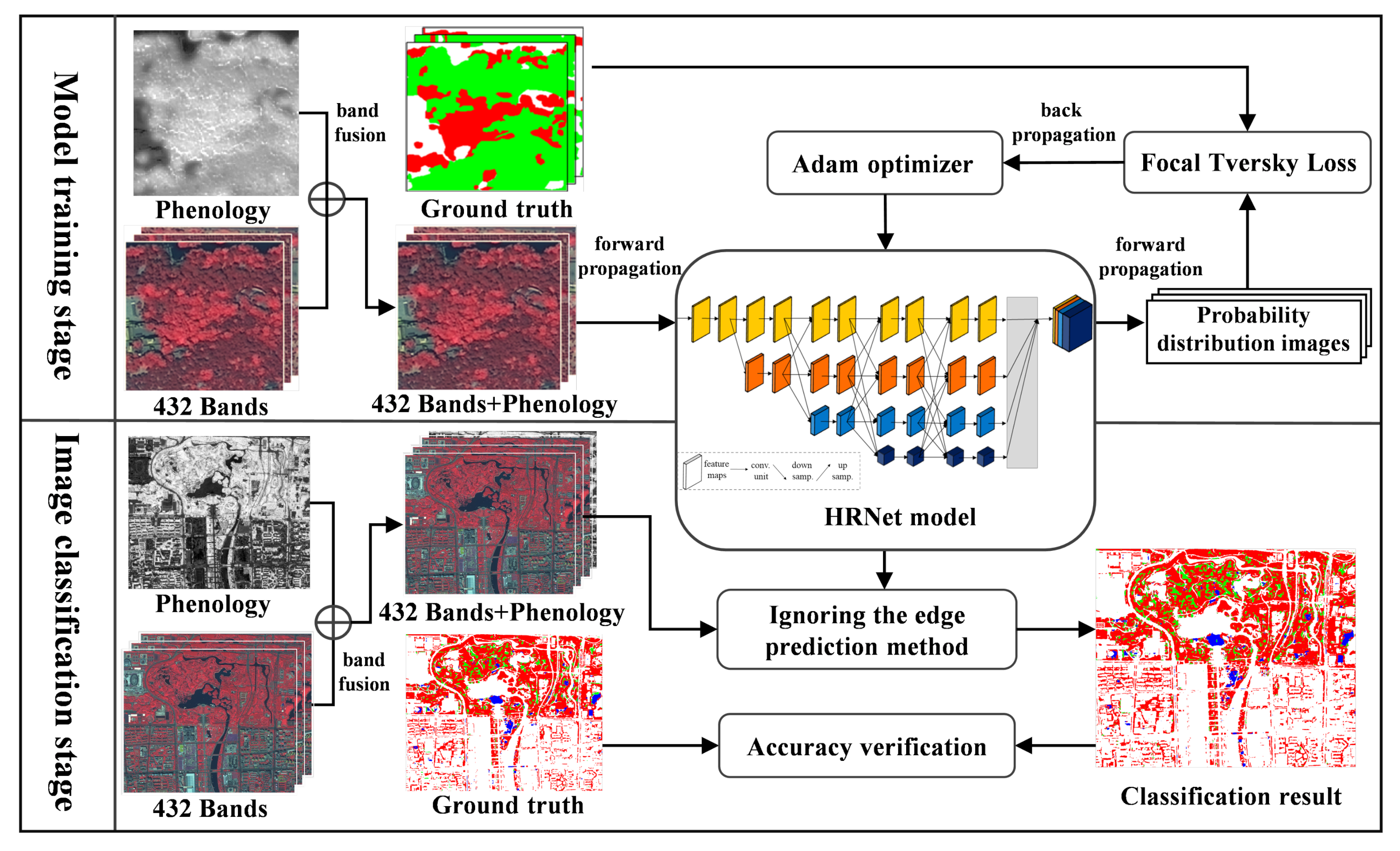
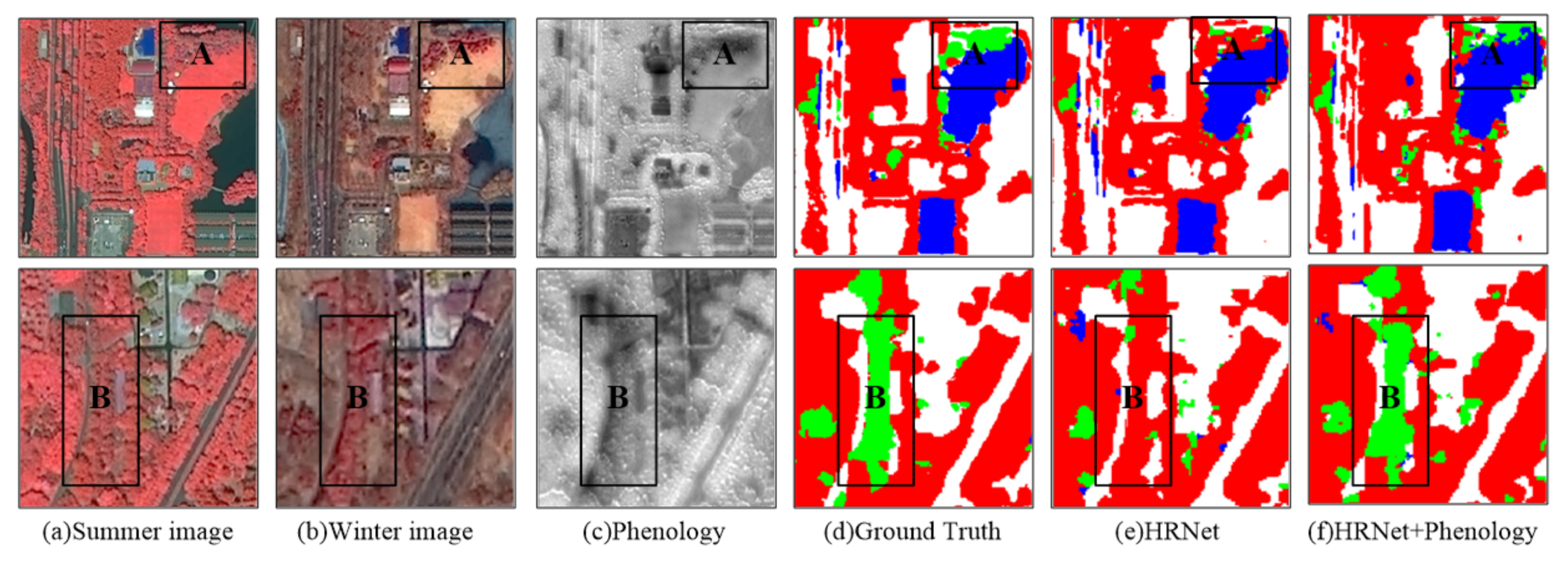
This paper proposed introducing phenological features into deep learning urban green space classification research. The experimental results show that the addition of phenological features can improve the richness of HRNet model learning, optimize the classification results, and eliminate the small misclassification phenomenon, proving that vegetation phenology is very useful in enhancing urban vegetation classification.
(2)
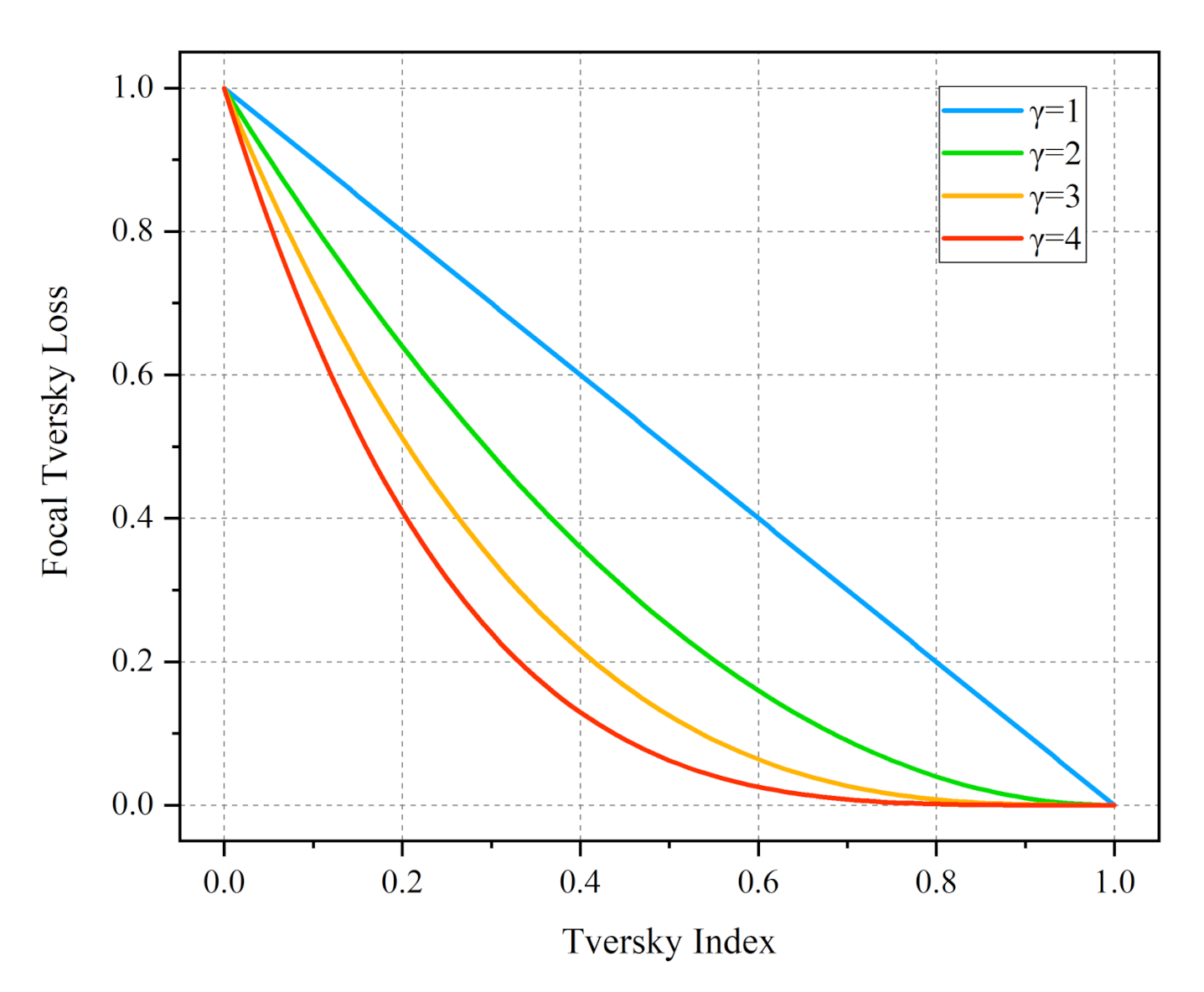
This paper proved that Focal Tversky Loss is better than Cross Entropy Loss, Dice Loss, and Tversky Loss by using the GF-2 Beijing urban green space dataset. The Focal Tversky Loss can reduce data imbalance in the classification task and improve urban green space classification accuracy.
(3)
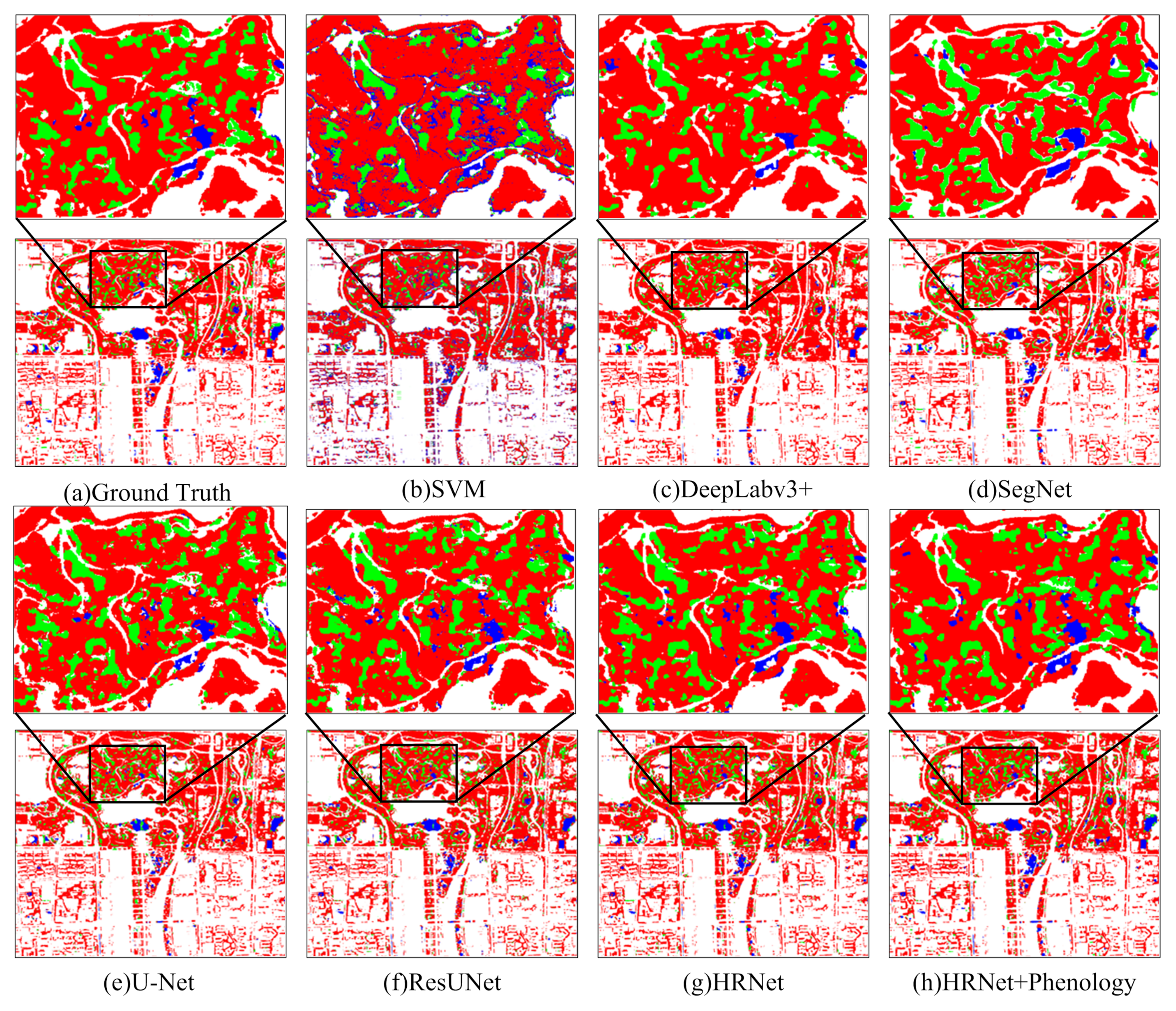
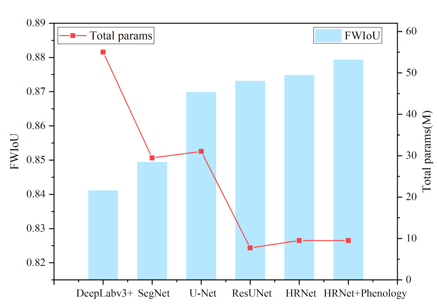
We compared HRNet with other convolutional neural network models, including SegNet, DeepLabv3+, U-Net, and ResUNet. The results show that our method performed well in urban green space classification.

2. Research Area and Data Source

2.1. Study Area

As China’s capital, Beijing attaches great importance to the development of the “green concept”. In 2019, Beijing built 803 hectares of urban green space, built 24 urban leisure parks, 13 natural urban forests, and approximately 60 pocket parks and micro-green spaces, which increased the urban green coverage to 48.46% [48]. While 2020 is the decisive period for building a moderately prosperous society in all respects, Beijing plans to build 700 hectares of urban green space, 41 leisure parks, 13 urban forests, and 50 pocket parks and micro-green spaces. The coverage rate of urban greening will be 48.5% [49].

2.1.1. Classification of Urban Green Space

The research object of this paper is Beijing urban green space. Beijing is a typical temperate continental monsoon climate, which is mainly planted in warm temperate deciduous broad-leaved forest and temperate coniferous forest. The species structure is diverse, and the four seasons are distinct. Affected by climate, in the growing season from late spring to early autumn, the trees are overgrown, and the grass is luxuriant. The content of chlorophyll in leaves increases, which absorbs red and blue light, reflecting green light, showing the green landscape of the city. When the temperature decreased from late autumn to early spring, the chlorophyll content decreased, and carotenoid content increased. The leaves absorb the blue and green light and reflect the yellow light, showing a different urban landscape. According to the vegetation phenology, the urban vegetation types in Beijing are divided into evergreen trees, deciduous trees, and grassland.

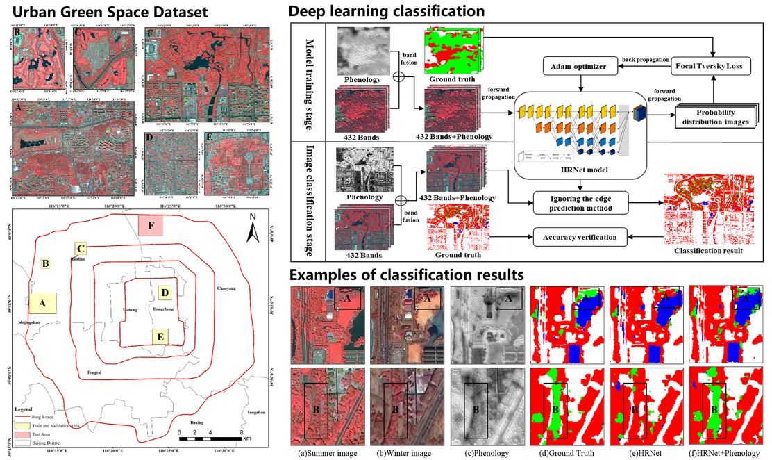
2.1.2. Training and Validation Area

Five sample areas were selected as the training data and validation data in the Fifth Ring Road District of Beijing (Figure 1). The sample areas include two urban parks (Laoshan urban leisure park and Temple of Heave Park), two golf courses (Xiangshan golf course and Wanliu golf course), and one residential area (Zhangzizhong Road residential area). The urban green space of the five sample areas is typical and representative. Among them, Laoshan urban leisure park, with the sample area of 9.29 km 2 , is located in the southeast of Shijingshan District, with rich vegetation types. Temple of Heaven Park, with the sample area of 4 km 2 , is located in the south of Beijing, surrounded by royal gardens. A large number of evergreen tree species are planted, such as ancient pine. Xiangshan golf course and Wanliu golf course, with the sample area of 1.56 km 2 and 2.42 km 2 , are located in Haidian District. They are two large golf courses with large grassland. Zhangzizhong Road residential area, with the sample area of 3.18 km 2 , is located in Dongcheng District of Beijing, with street trees and fragmentary green space between dense buildings.

2.1.3. Test Area

In addition, the Olympic Park area was selected as the test area in order to test the effectiveness of the proposed method for urban green space classification (Figure 2). The Olympic Park is located in Chaoyang District of Beijing. The sample area is 8.26 km 2 . The northern part is the Olympic Forest Park, with a greening coverage rate of 95.61%. It is rich in forest resources, mainly evergreen trees and deciduous trees. The southern part is the central square and urban built-up area, surrounded by landscape belt. Therefore, the Olympic Park has enough vegetation species and it can be used as the test area in order to verify the classification effect of different types of green space.

2.2. Data Source and Data Preprocessing

2.2.1. Satellite Image

The primary research data of this paper is GaoFen-2 satellite images (the data were obtained from the China Resources Satellite Application Center in February 2019 and June 2019). The GF-2 PMS sensor has a panchromatic band of 1 m spatial resolution and four multi-spectral bands of 4 m spatial resolution. The data processing includes orthographic correction, image fusion, image Mosaic, clipping, and bit depth adjustment. In order to better represent the vegetation features of urban green space, we use the standard false-color image combined with 4-3-2 bands to extract and classify urban green space.

2.2.2. Ground Truth

In this paper, six regions (five sample areas and one test area) were selected as train data, validation data, and test data in the Fifth Ring Road District of Beijing. The six regions basically cover typical types of urban green space in Beijing. Combining GF-2 and Google Earth high-resolution remote sensing images in summer and winter, we drew the outline of all types of green space in the image of the study area by manual visual interpretation and verified the interpretation results of three green space types through spot investigation in order to obtain the real label data of the surface. We masked the water area in the image to avoid the influence of wetland vegetation. The training dataset and validation dataset were obtained by data enhancement and clipping. There was no overlapping among the training dataset, verification dataset, and test dataset.

3. Methods

The whole process is mainly divided into two parts: model training and image classification, as shown in Figure 3. In the model training stage, the phenological features of urban green space were calculated using GF-2 images in February and June 2019. Subsequently, the value of phenological features were normalized into 8 bit and composed with the 4-3-2 standard false-color images as the fourth band image. After that, 1248 training datasets and 312 validation datasets were obtained by data enhancement and sliding window clipping for the superimposed image data and real labels. These training datasets were input into the HRNet model for feature learning in order to obtain the prediction probability distribution map. The model used Focal Tversky Loss to calculate the loss value between the predicted and true categories, and adopted the Adam optimization algorithm [50] to optimize the model parameters and reduce the loss value. The model was trained for 100 epochs.
In the image classification stage, the method of ignoring edge prediction [51] was adopted, which was to cut the silhouette with overlapping and adopting the strategy of ignoring edge when splicing. It can effectively solve the problem of insufficient edge pixel features. The predicted edge repetition rate was 35%.

3.1. Phenological Feature

Vegetation phenology can better reflect the response of different urban green space types to climate change. Vegetation phenological features can be obtained when combined with remote sensing images of different seasons, which is the essential basis for vegetation classification between evergreen and deciduous trees. This paper introduced the phenological information of urban green space in summer and winter to improve the richness of model feature learning. The trees are luxuriant in summer. In the remote sensing images, evergreen trees are generally dark red, while deciduous trees and grasslands are red and bright red, respectively. In winter, all of the deciduous trees wither, with the trunk or bare soil left on the original position, and the spectral information changes significantly. While the evergreen trees still stay dark red and some artificial grasslands still stay right red. In this paper, GF-2 multi-temporal remote sensing images are combined in order to extract the vegetation situation of the urban green space in different phases to improve urban green space classification accuracy.
NDVI is an important index to measure vegetation coverage and detect plant growth [11]. It can integrate the spectral information of vegetation, highlight the vegetation information on the image, and reduce the non-vegetation information. The difference between NDVI in summer and winter is used in order to reflect phenological characteristics, which can better characterize the spectral differences between evergreen and deciduous trees. The formula is as follows:
N D V I = N I R R N I R + R
P h e n o l o g y = N D V I s N D V I w
where NIR is the value in the near-infrared band, and R is the value in red band. NDVI s refers to the NDVI value in June, and NDVI w refers to the NDVI value in February.

3.2. HRNet Convolutional Neural Network

HRNet (High-Resolution Network) [42] was proposed by the Visual Computing Group of Microsoft Research Asia as a high-resolution deep neural network. With its unique structural framework, HRNet has excellent applications in attitude recognition, semantic segmentation, and target detection. HRNet is known as the “all-purpose backbone network structure”, where the network structure diagram is shown in Figure 4.

3.2.1. Parallel Multi-Resolution Subnetworks

The HRNet network structure is changed from the traditional serial connection high-low resolution convolution to parallel connection high-low resolution convolution. The network consists of four parallel multi-resolution subnets. The resolution and channel number of each subnet remain the same, but the resolutions among the parallel subnets are different. These parallel multi-resolution subnets learn rich features by keeping high resolution throughout the whole process and exchanging multiple messages for high- and low-resolution representations. It can effectively avoid the loss that is caused by the low-resolution feature to restore the high-resolution feature in serial connection in order to maintain the high-resolution feature of the image in the whole process.

3.2.2. Repeated Multi-Scale Fusion

The second advantage of HRNet is that it takes advantage of repeated multi-scale fusion [42]. Exchange units are introduced across parallel subnets, so that each subnet can repeatedly receive information from other parallel subnets. Therefore, low-resolution features of the same depth and similar level can be used to enhance the expression of high-resolution features. To generate low-resolution and high-level representations from high-resolution, we adopt strided 3 × 3 convolutions for downsampling. From low-resolution to high-resolution, we adopt the simple nearest neighbor sampling following a 1 × 1 convolution for aligning the number of channels. The same resolution takes the form of identity mapping.

3.2.3. Multi-Scale Features Concatenating

In the last stage of the network, the parallel four-branch subnets produce four feature maps with different resolutions. We adopted the multi-scale feature mosaic method of HRNetV2 proposed in the paper [42]. We carried out up-sampling for three low-resolution feature maps, and then concatenating with high-resolution features. This approach is more suitable for semantic segmentation tasks. It can not only maintain high-resolution features to reduce the loss of spatial accuracy, but also take into account the context information that is brought by low-resolution features.

3.3. Focal Tversky Loss

In deep learning, loss function plays an important role in evaluating the difference between the predicted value and true value of the model. By minimizing the loss function, the model can reach the convergence state and reduce the error of the model prediction value. Generally, the number of pixels in the background of remote sensing image is much larger than that of urban green space, and the number of pixels of deciduous trees in green space type is far greater than that of evergreen trees and grasslands. It leads to severe data imbalance in the task of urban green space classification. This problem leads to two results: (1) that the network model training could not obtain useful information more thoroughly and result in lower training efficiency; (2) the loss function of the model would be more affected by the separated background samples, which leads to a decrease in the accuracy of green space. The Tversky Loss [52] that was proposed by Seyed et al. can effectively solve the problem of data imbalance in medical image segmentation. Tversky Loss is essentially an improved model of dice loss, which is used to measure the similarity of sets. It can control the trade-off between false positive and false negative by adjusting α and β . The formula of Tversky index is as follows:
T L = 1 A B A B + α A B + β B A = 1 T P T P + α F P + β F N
where A is the true green space classification. B is the prediction result of the network. TP (True Positive) refers to the positive sample that is predicted to be a positive sample. TN (True Negative) refers to the negative sample that is predicted to be a negative sample. FP (False Positive) refers to the negative sample that is predicted to be a positive sample. FN (False Negative) refers to the positive sample that is predicted to be a negative sample. The super parameters and are used to control the balance between FP and FN. When α = β = 0.5 , Tversky Loss is Dice loss.
In order to better control the weight of easy and difficult samples, we used the Focal Loss idea proposed by Lin [53] and introduced a modulation coefficient ( 1 T L ) 1 / γ to the Tversky Loss function, with tunable focusing parameter γ > 0. By reducing the easily classified samples’ weight, the model can be trained to focus more on the hard-classified samples. The formula of Focal Tversky Loss is as follows:
F T L = c 1 T L 1 / γ

3.4. Evaluation Metrics

Three evaluation indicators were used in order to measure the effectiveness of the method: F1-Score, Overall Classification Accuracy (OA), and Frequency Weighted Intersection over Union (FWIoU) (Table 1). F1-Score, which is also known as the balanced score, is defined as the harmonic average of precision and recall rate. It is a common evaluation index for semantic segmentation. OA is a comprehensive evaluation index of classification results and represents the probability that the classification result for each pixel is consistent with the actual type of the label data. FWIoU [54], an improvement of Mean Intersection over Union (mIoU), sets weights for the frequency of each class and evaluate the comprehensive classification performance of the algorithm. The calculation equations for the indicators are as follows:
where N is the total pixel number of the image. C is the number of categories. x i i represents the pixel number of the category i that was correctly classified. x i j represents the pixel number of the category i that are wrongly divided into category j.

4. Results and Analysis

4.1. Comparative Experiments of Different Networks

4.1.1. Comparison of Classification Results of Different Networks

The image of Olympic Park was selected as the test dataset. In order to prove the effectiveness of the proposed method, it was compared with SVM, DeepLabv3+, SegNet, U-Net, ResUNet, and HRNet without phenological features. From the OA of the seven classification methods, the results of the proposed model in this article were the best. The OA was ranked from large to small: HRNet with phenology (93.24%) > HRNet (93.12%) > U-Net (92.81%) > ResUNet (92.8%) > SegNet (91.62%) > Deeplabv3+ (91.14%) > SVM (87.73%). Overall, deep learning methods had fewer mistakes and omissions than the SVM method. The SVM classification method cannot accurately identify the boundary of different urban green space categories, where the phenomenon of misclassification and omission is obvious. For instance, there was a large area of grassland in the central square of Olympic Forest Park, which was mistakenly divided into deciduous trees, while there were some scattered deciduous trees in residential areas that are mistakenly classified as grassland by SVM (Figure 5b). This issue can be attributed to two main factors. The first is the limitation of the classifier performance. The other is the difficulty in distinguishing the types of green space, which is due to the complication on the spectrum of the green space in the high-resolution images, such as “Same object with different spectrums” and “Foreign body in the same spectrum”.
The training results of different deep learning models were also different. It can be seen from Figure 5c that the classification results that were obtained by DeepLabv3+ ignored many small patches, and the accuracy of evergreen trees and grassland were low. The classification results of SegNet show that the edge of the object was smoother, and the detailed information of the edge was not processed properly (Figure 5d). The classification results of U-Net and ResUNet were much better, which was consistent with the results in the article [22]. The FWIoU of ResUNet results was 0.32% higher than that of U-Net. However, there were still small patches in these two methods (Figure 5e,f). It can be seen from Figure 5g that the classification results of HRNet were better than that of U-Net and ResUNet. The edge of deciduous trees was more consistent with the edge of the actual feature. The FWIoU of HRNet was 0.49% higher than that of U-Net.
The model in this paper had the best classification effect, and the detailed information on urban green space was better extracted. Among the three types of urban green space, the classification result of deciduous trees was the best, with an F1-Score of 0.9181. Deciduous trees were mainly distributed in urban parks, residential areas, and roadside trees. The classification result of evergreen trees in the three types was slightly inferior, with an F1-Score of 0.7248, being mainly distributed in urban parks. The F1-Score of grassland was 0.7588. Large grasslands were spread primarily on urban parks, while small grasslands were scattered in residential areas. The results of urban green space classification that were predicted by the method proposed in this paper were better. The OA was 93.24%, FWIoU was 87.93%. While the FWIoU was 0.45% higher than HRNet and 0.94% higher than U-Net (Table 2). It is proved that our model is advantageous in the classification of urban green space from high-resolution remote sensing images.

4.1.2. Comparison of Total Parameters of Different Networks

In addition to OA, F1-Score, and FWIoU, the total parameters of network is also a critical indicator for evaluating network efficiency. The more parameters the network has, the more memory it needs to occupy in the process of training and testing. Therefore, we further compared the total parameters of the proposed method and the other five methods.
Figure 6 shows the total parameters of different networks and the FWIoU evaluated on the Beijing Olympic Park dataset. Among all of the methods, the total parameters of ResUNet were the least, with 7.7 M. The total parameters of HRNet with and without phenological features were slightly larger than those of ResUNet (9.5 M). While the FWIoU that was obtained by HRNet with the phenological features was significantly higher than that of other methods. In contrast, DeepLabv3+, SegNet, and U-Net model training required more parameters and a lot of memory during training and testing.

4.2. Comparative Experiments of Different Loss Functions

We used different loss functions, including Cross Entropy Loss (CE), Tversky Loss (TL), and Focal Tversky Loss (FTL), in order to verify the effectiveness of Focal Tversky Loss.
First, five groups of tests were conducted on the Tversky Loss parameters α and β (Figure 7c–g). The results show that HRNet had the best classification effect when α = 0.8 and β = 0.2 . Compared with the Cross Entropy Loss, the overall classification accuracy of the Tversky Loss ( α = 0.8 , β = 0.2 ) was improved by 0.4%, FWIoU by 0.4%, deciduous trees, and evergreen trees by 0.05% and 2.53%. However, the F1-Score of grassland decreased to a certain extent by 0.0116 (Table 3).
Secondly, a modulation coefficient was used in order to make the model pay more attention to difficult-distinguished samples. Three cases of γ = 1 , 2 , 3 were tested (Figure 7h–j). It found that, when γ = 2 , the combination effect of HRNet and Focal Tversky Loss was the best, the OA reaches 93.12%, with 0.23% higher than Tversky Loss ( α = 0.8 , β = 0.2 ), 0.63% higher than Cross Entropy Loss ( α = 0.8 , β = 0.2 ). The FWIoU was 0.8748, 0.25% higher than Tversky Loss ( α = 0.8 , β = 0.2 ), and 0.65% higher than Cross Entropy Loss. When compared with Tversky Loss ( α = 0.8 , β = 0.2 ), the Focal Tversky Loss paid more attention to the hard samples, the F1-Score of deciduous trees and evergreen trees were increased by 0.38% and 0.9%, respectively, and grassland decreased to a certain extent (Table 3).

4.3. Comparative Experiments about Vegetation Phenology

We compared the HRNet model and Focal Tversky Loss ( α = 0.8 , β = 0.2 , γ = 2 ) with and without the phenological features in order to verify whether adding the phenological features can effectively improve the classification effect of the model. Figure 8 shows the results of two classification methods for A and B regions. There were two large areas of evergreen trees in regions A and B, which were green on the Ground Truth images (Figure 8d). The results show that large areas of evergreen trees (green) were wrongly classified as deciduous trees (red) in A and B regions with the HRNet without adding the phenological features. After adding the phenological features, the misclassification phenomenon was reduced. The large areas of evergreen trees were basically correctly classified and the edges of evergreen trees were more detailed, which was more consistent with the ground truth results. While some small and scattered evergreen trees were also classified although their boundaries were fuzzy. On the whole, the classification results of the HRNet model can be significantly improved by combining the phenological features of vegetation from multi-seasonal images with the remote sensing image of GF-2.

5. Discussion

5.1. Alleviation of Imbalanced Sample Classification by Introducing Focal Tversky Loss

The Focal Tversky Loss function ( α = 0.8 , β = 0.2 , γ = 2 ) had the highest classification accuracy among different loss functions in HRNet, as seen from Table 3. This can be attributed to the following factors: Cross Entropy Loss function adopts the competition mechanism in different classes, and only concerns about the accuracy of prediction probability for correct labels, which ignores the differences of incorrect labels and results in scattered learned features [55]. When background samples increase, HRNet will be occupied by more simple samples, which makes the model ignore the learning of urban green space samples. This is also the reason why the evergreen tree F1-Score is low. Dice Loss function is not conducive to the back-propagation of the training model and easy to cause parameter oscillation during training, so the classification accuracy is the worst [56]. Tversky Loss improves Dice Loss by a better compromise between precision and recall and emphasizes false negative, but still ignores difficult sample training [52].
Focal Tversky Loss adds a modulation coefficient γ into Tversky Loss function to concentrate on hard samples. When γ increases gradually, the modulating factor will gradually decrease, and the Focal Tversky Loss will focus more on the prediction with less accurate classification, as shown in Figure 9. Therefore, Focal Tversky Loss function can alleviate the imbalance of sample classification and improve the classification accuracy.
However, with the increase of γ , the over-inhibition of the model on the easily divided samples also affected the final classification accuracy. Therefore, it is necessary to find the most suitable value of γ . The results show that γ = 2 was the optimal parameter of our experiments. The training model can not only effectively enhance the training on deciduous trees samples and evergreen trees samples, but also not excessively restrain the accuracy of the background samples. When γ = 1 , the Focal Tversky Loss is Tversky Loss. When γ = 3 , the model over suppressed the easily separated samples, which resulted in the decline of F1-Score of deciduous trees, evergreen trees, and other category. It should be noted that the super parameter was increased by one in this paper, but there may be another better solution when the increment of γ is set to a lower value.

5.2. Improvement of Urban Green Space Classification by Adding Vegetation Phenology into HRNet

In this paper, vegetation phenology was added into the HRNet model in order to reflect the changes of plants. Table 4 shows the accuracy of the HRNet model with and without vegetation phenology. It can be seen from Table 4 that the addition of phenological features can improve the classification results of the urban green space of HRNet model, especially that the classification accuracy of evergreen trees was 4.77% higher than that of the method without phenological features. When compared with the results of HRNet without phenological features, the F1-Score of deciduous trees and grassland were increased by 0.48% and 3.93%, respectively. The increasing rate of the average F1-Score was 2.00%, the OA increased from 93.12% to 93.24%, and FWIoU increased from 0.8748 to 0.8793. The experimental results show that the addition of phenological features for HRNet model training can provide the phenology of urban green space in order to improve image classification accuracy, which is consistent with previous studies on urban green space classification while using the object-oriented method [45,47].
The improvement of classification accuracy can be explained through the remote sensing images. In summer, vegetation grows vigorously and spongy tissue in the leaves of broad-leaved trees strongly reflects near-infrared light. Based on organizational structure characteristics of plant leaves, some deciduous broad-leaved trees, and evergreen conifers could be distinguished. However, it is still difficult to distinguish the boundary evergreen trees from deciduous trees by visual inspection. Winter is the dormant period of deciduous vegetation, while evergreen trees still grow vigorously. Besides, the chlorophyll content of grassland in winter is also decreasing, and the color is also changed. Therefore, remote sensing images during different periods can better reflect the changes in vegetation spectral characteristics with plant physiology and identify the different types of green space.
However, we found that the accuracy of model promotion was not high. Based on this problem, the main reason could be attributed to the imbalance of the area proportion of different vegetation types in the Olympic Park sample area. The area of non-vegetation area accounts for 60.98% of the total area, so the classification effect of non-vegetation area has a great impact on the OA. The number of pixels correctly divided into deciduous trees was increased by 58,044 when using HRNet with phenology feature, but the pixels of deciduous trees account for 33.91% of the total sample pixels, so the F1-Score only increased by 0.0044. The number of pixels correctly divided into evergreen trees was increased by 46,448, and the area of evergreen trees accounted for 3.36% of the total area. Hence, the F1-Score was increased by 0.033, from 0.6918 to 0.7248, with an increase rate of 4.77%. The number of pixels correctly divided into grassland was increased by 6194, but the proportion of grassland area was only 1.75% of the total area. Therefore, the F1-Score of grassland increased from 0.7301 to 0.7588, with an increase rate of 3.93%. It can be observed that the imbalance of data categories will affect the final classification accuracy evaluation. The vegetation coverage and vegetation types in the test sample area are not balanced, which leads to the largest background category playing a leading role in the final classification results, so that the improvement of vegetation classification accuracy has little impact on the final classification accuracy.

6. Conclusions

In this paper, a deep learning classification method for urban green space that is based on the Focal Tversky Loss and phenological features is constructed to solve the problems of incomplete extraction of green space types and inaccurate boundary extraction from high-resolution remote sensing images. The results show that HRNet combined with phenology has a good classification effect on the urban green space classification in Beijing. Simultaneously, Focal Tversky Loss can better improve the classification imbalance of urban green space dataset and make the model pay more attention to the hard classify samples. The classification effect is better than the Cross Entropy Loss. The selection of super parameters α , β , and γ should be combined with different datasets to determine the optimal threshold value. In this paper, α = 0.8 , β = 0.2 , and γ = 2 are selected to achieve the best classification effect. In addition, it proved that vegetation phenology is very useful in improving urban vegetation classification. When the phenological features are applied to classification, the overall classification accuracy of the model is improved from 93.12% to 93.24%, and FWIoU is improved from 0.8748 to 0.8793. In particular, the F1-Score of deciduous trees, evergreen trees, and grassland predicted by our model increased by 0.48%, 4.77%, and 3.93% than the model without phenological features. It is proved that the combination of phenological features and high-resolution remote sensing images is an effective method for improving the urban green space classification accuracy.
In this paper, Beijing was selected as the research area, which belongs to the middle latitude region and the vegetation type is mainly deciduous broad-leaved forest. Hence, the proportion of evergreen trees in Beijing is much lower, which results in less impact of phenological features on the final classification accuracy. The follow-up study can be expanded to the low latitude areas with rich vegetation types and balanced distribution, so as to verify the generalization of the model and effect of green space classification.

Author Contributions

Z.X. wrote the manuscript and designed the comparative experiments; Y.Z. and S.W. (Shixin Wang) supervised the study and revised the manuscript; L.W. provided GF-2 data, revised the manuscript and gave comments and suggestions to the manuscript; F.L. and S.W. (Shicheng Wang) gave suggestions to the manuscript; Z.W. assisted Z.X. in designing the architecture and conducting experiments. All authors have read and agreed to the published version of the manuscript.

Funding

This research was funded by the National Key R&D Program of China (Grant number: 2017YFB0504000) and the project “Regional Eco-environment Monitoring System” (Grant number: 200266).

Acknowledgments

The authors would like to thank the editors and the reviewers for their valuable suggestions.

Conflicts of Interest

The authors declare no conflict of interest.

References

  1. Yang, J.; McBride, J.; Zhou, J.; Sun, Z. The urban forest in Beijing and its role in air pollution reduction. Urban For. Urban Green. 2005, 3, 65–78. [Google Scholar] [CrossRef]
  2. Dwivedi, P.; Rathore, C.S.; Dubey, Y. Ecological benefits of urban forestry: The case of Kerwa Forest Area (KFA), Bhopal, India. Appl. Geogr. 2009, 29, 194–200. [Google Scholar] [CrossRef]
  3. Thompson, C.W.; Roe, J.; Aspinall, P.; Mitchell, R.; Clow, A.; Miller, D. More green space is linked to less stress in deprived communities: Evidence from salivary cortisol patterns. Landsc. Urban Plan. 2012, 105, 221–229. [Google Scholar] [CrossRef] [Green Version]
  4. Xiao, R.; Zhou, Z.; Wang, P.; Ye, Z.; Guo, E.; Ji, G. Application of 3S technologies in urban green space ecology. Chin. J. Ecol. 2004, 23, 71–76. [Google Scholar]
  5. Groenewegen, P.P.; Van den Berg, A.E.; De Vries, S.; Verheij, R.A. Vitamin G: Effects of green space on health, well-being, and social safety. BMC Public Health 2006, 6, 149. [Google Scholar] [CrossRef] [Green Version]
  6. Seto, K.C.; Woodcock, C.; Song, C.; Huang, X.; Lu, J.; Kaufmann, R. Monitoring land-use change in the Pearl River Delta using Landsat TM. Int. J. Remote Sens. 2002, 23, 1985–2004. [Google Scholar] [CrossRef]
  7. Yuan, F.; Sawaya, K.E.; Loeffelholz, B.C.; Bauer, M.E. Land cover classification and change analysis of the Twin Cities (Minnesota) Metropolitan Area by multitemporal Landsat remote sensing. Remote Sens. Environ. 2005, 98, 317–328. [Google Scholar] [CrossRef]
  8. Portillo-Quintero, C.; Sanchez, A.; Valbuena, C.; Gonzalez, Y.; Larreal, J. Forest cover and deforestation patterns in the Northern Andes (Lake Maracaibo Basin): A synoptic assessment using MODIS and Landsat imagery. Appl. Geogr. 2012, 35, 152–163. [Google Scholar] [CrossRef]
  9. Hurd, J.D.; Wilson, E.H.; Lammey, S.G.; Civco, D.L. Characterization of forest fragmentation and urban sprawl using time sequential Landsat imagery. In Proceedings of the ASPRS Annual Convention; Citeseer: St. Louis, MO, USA, 2001; Volume 21. [Google Scholar]
  10. Miller, M.D. The impacts of Atlanta’s urban sprawl on forest cover and fragmentation. Appl. Geogr. 2012, 34, 171–179. [Google Scholar] [CrossRef]
  11. Tucker, C.J.; Pinzon, J.E.; Brown, M.E.; Slayback, D.A.; Pak, E.W.; Mahoney, R.; Vermote, E.F.; El Saleous, N. An extended AVHRR 8-km NDVI dataset compatible with MODIS and SPOT vegetation NDVI data. Int. J. Remote Sens. 2005, 26, 4485–4498. [Google Scholar] [CrossRef]
  12. Huete, A.R. A soil-adjusted vegetation index (SAVI). Remote Sensing of Environment. Remote Sens. Environ. 1988, 25, 295–309. [Google Scholar] [CrossRef]
  13. Huete, A.; Didan, K.; Miura, T.; Rodriguez, E.P.; Gao, X.; Ferreira, L.G. Overview of the radiometric and biophysical performance of the MODIS vegetation indices. Remote Sens. Environ. 2002, 83, 195–213. [Google Scholar] [CrossRef]
  14. Yao, F.; Luo, J.; Shen, Z.; Dong, D.; Yang, K. Automatic urban vegetation extraction method using high resolution imagery. J. Geo Inf. Sci. 2016, 18, 248–254. [Google Scholar]
  15. Sirirwardane, M.; Gunatilake, J.; Sivanandarajah, S. Study of the Urban Green Space Planning Using Geographic Information Systems and Remote Sensing Approaches for the City of Colombo, Sri Lanka. In Geostatistical and Geospatial Approaches for the Characterization of Natural Resources in the Environment; Springer: New Delhi, India, 2016; pp. 797–800. [Google Scholar]
  16. Kranjčić, N.; Medak, D.; Župan, R.; Rezo, M. Machine learning methods for classification of the green infrastructure in city areas. ISPRS Int. J. Geo-Inf. 2019, 8, 463. [Google Scholar] [CrossRef] [Green Version]
  17. Jianhui, X.; Ya, S. Study of Urban Green Space Surveying Based on High Resolution Images of Remote Sensing. Resour. Dev. Mark. 2010, 26, 291–294. [Google Scholar]
  18. Qian, Y.; Zhou, W.; Yu, W.; Pickett, S.T. Quantifying spatiotemporal pattern of urban greenspace: New insights from high resolution data. Landsc. Ecol. 2015, 30, 1165–1173. [Google Scholar] [CrossRef]
  19. Huang, H.P.; Wu, B.F.; Li, M.M.; Zhou, W.F.; Wang, Z.W. Detecting urban vegetation efficiently with high resolution remote sensing data. J. Remote Sens. Beijing 2004, 8, 68–74. [Google Scholar]
  20. Meng, Q.Y.; Chen, X.; Sun, Y.X.; Wu, J. Urban building green environment index based on LiDAR and multispectral data. Chin. J. Ecol. 2019, 38, 3221. [Google Scholar]
  21. Peng, C.; Li, Y.; Jiao, L.; Chen, Y.; Shang, R. Densely based multi-scale and multi-modal fully convolutional networks for high-resolution remote-sensing image semantic segmentation. IEEE J. Sel. Top. Appl. Earth Obs. Remote Sens. 2019, 12, 2612–2626. [Google Scholar] [CrossRef]
  22. Xu, Z.; Zhou, Y.; Wang, S.; Wang, L.; Wang, Z. U-Net for urban green space classification in GF-2 remote sensing images. J. Image Graph. 2021, in press. [Google Scholar] [CrossRef]
  23. Zhou, M.; Shi, Z.; Ding, H. Aircraft classification in remote-sensing images using convolutional neural networks. J. Image Graph. 2017, 22, 702–708. [Google Scholar]
  24. Haiwei, H.; Haizhong, Q.; Limin, X.; Peixiang, D. Interchange Recognition Method Based on CNN. Acta Geod. Cartogr. Sin. 2018, 47, 385. [Google Scholar]
  25. Hamaguchi, R.; Hikosaka, S. Building detection from satellite imagery using ensemble of size-specific detectors. In Proceedings of the 2018 IEEE/CVF Conference on Computer Vision and Pattern Recognition Workshops (CVPRW), Salt Lake City, UT, USA, 18–22 June 2018; pp. 223–2234. [Google Scholar]
  26. Zhao, K.; Kang, J.; Jung, J.; Sohn, G. Building Extraction From Satellite Images Using Mask R-CNN With Building Boundary Regularization. In Proceedings of the IEEE Conference on Computer Vision and Pattern Recognition (CVPR) Workshops, Salt Lake City, UT, USA, 18–22 June 2018; pp. 247–251. [Google Scholar]
  27. Yang, X.; Sun, H.; Fu, K.; Yang, J.; Sun, X.; Yan, M.; Guo, Z. Automatic ship detection in remote sensing images from google earth of complex scenes based on multiscale rotation dense feature pyramid networks. Remote Sens. 2018, 10, 132. [Google Scholar] [CrossRef] [Green Version]
  28. Ghosh, A.; Ehrlich, M.; Shah, S.; Davis, L.S.; Chellappa, R. Stacked U-Nets for Ground Material Segmentation in Remote Sensing Imagery. In Proceedings of the IEEE Conference on Computer Vision and Pattern Recognition (CVPR) Workshops, Salt Lake City, UT, USA, 18–22 June 2018; pp. 257–261. [Google Scholar]
  29. Pascual, G.; Seguí, S.; Vitrià, J. Uncertainty Gated Network for Land Cover Segmentation. In Proceedings of the IEEE Conference on Computer Vision and Pattern Recognition (CVPR) Workshops, Salt Lake City, UT, USA, 19–21 June 2018; pp. 276–279. [Google Scholar]
  30. Zhang, X.; Chen, X.; Li, F.; Yang, T. Change Detection Method for High Resolution Remote Sensing Images Using Deep Learning. Acta Geod. Cartogr. Sin. 2017, 46, 999. [Google Scholar]
  31. Ji, S.; Xu, W.; Yang, M.; Yu, K. 3D convolutional neural networks for human action recognition. IEEE Trans. Pattern Anal. Mach. Intell. 2012, 35, 221–231. [Google Scholar] [CrossRef] [Green Version]
  32. Panboonyuen, T.; Jitkajornwanich, K.; Lawawirojwong, S.; Srestasathiern, P.; Vateekul, P. Road segmentation of remotely-sensed images using deep convolutional neural networks with landscape metrics and conditional random fields. Remote Sens. 2017, 9, 680. [Google Scholar] [CrossRef] [Green Version]
  33. Wu, G.; Shao, X.; Guo, Z.; Chen, Q.; Yuan, W.; Shi, X.; Xu, Y.; Shibasaki, R. Automatic building segmentation of aerial imagery using multi-constraint fully convolutional networks. Remote Sens. 2018, 10, 407. [Google Scholar] [CrossRef] [Green Version]
  34. LeCun, Y.; Bottou, L.; Bengio, Y.; Haffner, P. Gradient-based learning applied to document recognition. Proc. IEEE 1998, 86, 2278–2324. [Google Scholar] [CrossRef] [Green Version]
  35. Krizhevsky, A.; Sutskever, I.; Hinton, G.E. Imagenet classification with deep convolutional neural networks. Commun. ACM 2017, 60, 84–90. [Google Scholar] [CrossRef]
  36. Simonyan, K.; Zisserman, A. Very Deep Convolutional Networks for Large-Scale Image Recognition. arXiv 2014, arXiv:1409.1556. [Google Scholar]
  37. Szegedy, C.; Liu, W.; Jia, Y.; Sermanet, P.; Reed, S.; Anguelov, D.; Erhan, D.; Vanhoucke, V.; Rabinovich, A. Going deeper with convolutions. In Proceedings of the IEEE Conference on Computer Vision and Pattern Recognition (CVPR), Boston, MA, USA, 8–10 June 2015; pp. 1–9. [Google Scholar]
  38. He, K.; Zhang, X.; Ren, S.; Sun, J. Deep residual learning for image recognition. In Proceedings of the IEEE Conference on Computer Vision and Pattern Recognition (CVPR), Las Vegas, NV, USA, 27–30 June 2016; pp. 770–778. [Google Scholar]
  39. Huang, G.; Liu, Z.; Van Der Maaten, L.; Weinberger, K.Q. Densely connected convolutional networks. In Proceedings of the IEEE Conference on Computer Vision and Pattern Recognition (CVPR), Honolulu, HI, USA, 22–25 July 2017; pp. 4700–4708. [Google Scholar]
  40. Badrinarayanan, V.; Kendall, A.; Cipolla, R. Segnet: A deep convolutional encoder-decoder architecture for image segmentation. IEEE Trans. Pattern Anal. Mach. Intell. 2017, 39, 2481–2495. [Google Scholar] [CrossRef] [PubMed]
  41. Ronneberger, O.; Fischer, P.; Brox, T. U-net: Convolutional networks for biomedical image segmentation. In International Conference on Medical Image Computing and Computer-Assisted Intervention; Springer: Munich, Germany, 2015; pp. 234–241. [Google Scholar]
  42. Sun, K.; Xiao, B.; Liu, D.; Wang, J. Deep high-resolution representation learning for human pose estimation. In Proceedings of the IEEE/CVF Conference on Computer Vision and Pattern Recognition (CVPR), Long Beach, CA, USA, 16–20 June 2019; pp. 5693–5703. [Google Scholar]
  43. Su-Ting, C.; Hui, Y. High resolution remote sensing image classification based on multi-scale and multi-feature fusion. Chin. J. Quantum Electron. 2016, 33, 420. [Google Scholar]
  44. Sun, W.; Wang, R. Fully convolutional networks for semantic segmentation of very high resolution remotely sensed images combined with DSM. IEEE Geosci. Remote Sens. Lett. 2018, 15, 474–478. [Google Scholar] [CrossRef]
  45. Senf, C.; Leitão, P.J.; Pflugmacher, D.; van der Linden, S.; Hostert, P. Mapping land cover in complex Mediterranean landscapes using Landsat: Improved classification accuracies from integrating multi-seasonal and synthetic imagery. Remote Sens. Environ. 2015, 156, 527–536. [Google Scholar] [CrossRef]
  46. Ulsig, L.; Nichol, C.J.; Huemmrich, K.F.; Landis, D.R.; Middleton, E.M.; Lyapustin, A.I.; Mammarella, I.; Levula, J.; Porcar-Castell, A. Detecting inter-annual variations in the phenology of evergreen conifers using long-term MODIS vegetation index time series. Remote Sens. 2017, 9, 49. [Google Scholar] [CrossRef] [Green Version]
  47. Yan, J.; Zhou, W.; Han, L.; Qian, Y. Mapping vegetation functional types in urban areas with WorldView-2 imagery: Integrating object-based classification with phenology. Urban For. Urban Green. 2018, 31, 230–240. [Google Scholar] [CrossRef]
  48. Beijing Gardening and Greening Bureau. Work Summary in 2019 and Work Plan in 2020 of Beijing Gardening and Greening Bureau. Available online: http://yllhj.beijing.gov.cn/zwgk/ghxx/jhzj/202002/t20200227_1670249.shtml (accessed on 3 November 2020).
  49. Beijing Gardening and Greening Bureau. Notice on Printing and Distributing the Key Points of Urban Greening Work in 2020. Available online: http://yllhj.beijing.gov.cn/zwgk/fgwj/qtwj/202001/t20200121_1619893.shtml (accessed on 3 November 2020).
  50. Nhu, V.H.; Hoang, N.D.; Nguyen, H.; Ngo, P.T.T.; Bui, T.T.; Hoa, P.V.; Samui, P.; Bui, D.T. Effectiveness assessment of keras based deep learning with different robust optimization algorithms for shallow landslide susceptibility mapping at tropical area. Catena 2020, 188, 104458. [Google Scholar] [CrossRef]
  51. Wang, Z.; Zhou, Y.; Wang, S.; Wang, F.; Xu, Z. House building extraction from high resolution remote sensing image based on IEU-Net. J. Remote Sens. 2021, in press. [Google Scholar] [CrossRef]
  52. Salehi, S.S.M.; Erdogmus, D.; Gholipour, A. Tversky loss function for image segmentation using 3D fully convolutional deep networks. In International Workshop on Machine Learning in Medical Imaging; Springer: Quebec City, QC, Canada, 2017; pp. 379–387. [Google Scholar]
  53. Lin, T.Y.; Goyal, P.; Girshick, R.; He, K.; Dollár, P. Focal loss for dense object detection. In Proceedings of the IEEE International Conference on Computer Vision (ICCV), Venice, Italy, 22–29 October 2017; pp. 2980–2988. [Google Scholar]
  54. Peng, Y.; Zhang, Z.; He, G.; Wei, M. An improved grabcut method based on a visual attention model for rare-earth ore mining area recognition with high-resolution remote sensing images. Remote Sens. 2019, 11, 987. [Google Scholar] [CrossRef] [Green Version]
  55. Zhang, Z.; Sabuncu, M. Generalized cross entropy loss for training deep neural networks with noisy labels. In Proceedings of the Advances in Neural Information Processing Systems (NeurIPS), Montréal, QC, Canada, 3–8 December 2018; pp. 8778–8788. [Google Scholar]
  56. Milletari, F.; Navab, N.; Ahmadi, S.A. V-net: Fully convolutional neural networks for volumetric medical image segmentation. In Proceedings of the 2016 Fourth International Conference on 3D Vision (3DV), Stanford, CA, USA, 25–28 October 2016; pp. 565–571. [Google Scholar]
Figure 1. Study Area. Region A is Laoshan urban leisure park. Region B is Xiangshan golf course. Region C is Wanliu golf course. Region D is Zhangzizhong Road residential. Region E is Temple of Heave Park. Region F is Olympic Park. Region A–E are the train and validation data, and Region F is the test data.
Remotesensing 12 03845 g001
Figure 2. Test area and Ground truth.
Remotesensing 12 03845 g002
Figure 3. Experimental flow chart.
Remotesensing 12 03845 g003
Figure 4. HRNet structure diagram.
Remotesensing 12 03845 g004
Figure 5. Comparison of the results of different classification methods.
Remotesensing 12 03845 g005
Figure 6. Comparison of Frequency Weighted Intersection over Union (FWIoU) and total parameters of different networks. The bar represents FWIoU evaluated on the Beijing Olympic Park dataset, and the broken line represents the total parameters of different networks (M).
Remotesensing 12 03845 g006
Figure 7. Comparison of the results of HRNet with Cross Entropy Loss, Tversky Loss, and Focal Tversky Loss.
Remotesensing 12 03845 g007
Figure 8. Comparison of the results of the methods with and without the phenology feature.
Remotesensing 12 03845 g008
Figure 9. The trend diagram of Focal Tversky Loss under different γ values (The Focal Tversky Loss focuses training on difficult samples (Tversky index < 0.5) and suppresses the contribution of simple samples (Tversky index > 0.5) to the loss function).
Remotesensing 12 03845 g009
Table 1. Evaluation Metrics.
Evaluation MetricsFormula
F 1 Score = 2 × P r e c i s i o n × R e c a l l P r e c i s i o n + R e c a l l
F1-Score P r e c i s i o n = T P T P + F P
R e c a l l = T P T P + F N
OA O A = i = 1 n x i i N
FWIoU F W I o U = 1 i = 0 C j = 0 C x i j i = 0 C j = 0 C x i j x i i j = 0 C x i j + j = 0 C x j i x i i
Table 2. Comparison of the accuracy of different classification methods.
PlanDeciduous TreesEvergreen TreesGrasslandOtherAverageOAFWIoU
F1-ScoreF1-ScoreF1-ScoreF1-ScoreF1-Score
SVM0.86350.52020.17690.94860.627387.73%82.13%
DeepLabv3+0.88750.53780.63610.94850.752591.14%84.11%
SegNet0.89370.6140.73070.94890.796891.62%84.94%
U-Net0.91020.68160.70150.95740.812792.81%86.99%
ResUNet0.91090.65410.73630.96010.8153592.80%87.31%
HRNet0.91370.69180.73010.9590.823793.12%87.48%
HRNe+Phenology0.91810.72480.75880.9590.840293.24%87.93%
Table 3. Comparison of the accuracy of HRNet with Cross Entropy Loss, Tversky Loss, and Focal Tversky Loss.
PlanDeciduous TreesEvergreen TreesGrasslandOtherAverageOAFWIoU
F1-ScoreF1-ScoreF1-ScoreF1-ScoreF1-Score
HRNet (CE)0.90940.65750.74940.95620.8181250.92490.8683
HRNet (DL, α = 0.5 , β = 0.5 )0.90150.66140.71670.95690.8091250.92370.864
HRNet (TL, α = 0.6 , β = 0.4 )0.90880.6570.72120.9590.81150.92640.8705
HRNet (TL, α = 0.7 , β = 0.3 )0.90910.66940.7020.95850.809750.92820.8702
HRNet (TL, α = 0.8 , β = 0.2 )0.90990.68280.73780.95890.822350.92890.8723
HRNet (TL, α = 0.9 , β = 0.1 )0.9060.65430.76080.95790.819750.9250.8684
HRNet (FT, α = 0.8 , β = 0.2 , γ = 2 )0.91370.69180.73010.9590.823650.93120.8748
HRNet (FT, α = 0.8 , β = 0.2 , γ = 3 )0.90560.63910.75520.95710.814250.92330.8666
Table 4. Comparison of the accuracy of the methods with and without the phenology feature.
PlanDeciduous TreesEvergreen TreesGrasslandOtherAverageOAFWIoU
F1-ScoreF1-ScoreF1-ScoreF1-ScoreF1-Score
HRNet0.91370.69180.73010.95900.82370.93120.8748
HRNe+Phenology0.91810.72480.75880.95900.84020.93240.8793
The loss function adopts Focal Tversky Loss, α = 0.8 , β = 0.2 , γ = 2 .
Publisher’s Note: MDPI stays neutral with regard to jurisdictional claims in published maps and institutional affiliations.

