Applying Deep Learning to Clear-Sky Radiance Simulation for VIIRS with Community Radiative Transfer Model—Part 2: Model Architecture and Assessment

Abstract

A fully connected “deep” neural network algorithm with the Community Radiative Transfer Model (FCDN_CRTM) is proposed to explore the efficiency and accuracy of reproducing the Visible Infrared Imaging Radiometer Suite (VIIRS) radiances in five thermal emission M (TEB/M) bands. The model was trained and tested in the nighttime global ocean clear-sky domain, in which the VIIRS observation minus CRTM (O-M) biases have been well validated in recent years. The atmosphere profile from the European Centre for Medium-Range Weather Forecasts (ECMWF) and sea surface temperature (SST) from the Canadian Meteorology Centre (CMC) were used as FCDN_CRTM input, and the CRTM-simulated brightness temperatures (BTs) were defined as labels. Six dispersion days’ data from 2019 to 2020 were selected to train the FCDN_CRTM, and the clear-sky pixels were identified by an enhanced FCDN clear-sky mask (FCDN_CSM) model, which was demonstrated in Part 1. The trained model was then employed to predict CRTM BTs, which were further validated with the CRTM BTs and the VIIRS sensor data record (SDR) for both efficiency and accuracy. With iterative refinement of the model design and careful treatment of the input data, the agreement between the FCDN_CRTM and the CRTM was generally good, including the satellite zenith angle and column water vapor dependencies. The mean biases of the FCDN_CRTM minus CRTM (F-C) were typically ~0.01 K for all five bands, and the high accuracy persisted during the whole analysis period. Moreover, the standard deviations (STDs) were generally less than 0.1 K and were consistent for approximately half a year, before they significantly degraded. The validation with VIIRS SDR data revealed that both the predicted mean biases and the STD of the VIIRS observation minus FCDN_CRTM (V-F) were comparable with the VIIRS minus direct CRTM simulation (V-C). Meanwhile, both V-F and V-C exhibited consistent global geophysical and statistical distribution, as well as stable long-term performance. Furthermore, the FCDN_CRTM processing time was more than 40 times faster than CRTM simulation. The highly efficient, accurate, and stable performances indicate that the FCDN_CRTM is a potential solution for global and real-time monitoring of sensor observation minus model simulation, particularly for high-resolution sensors.

1. Introduction

The Community Radiative Transfer Model (CRTM) was developed at the Joint Center for Satellite Data Assimilation (JCSDA). This fast radiative transfer model is used at the National Oceanic and Atmospheric Administration (NOAA) and in many institutes and universities, both nationally and internationally [1,2,3,4,5,6,7]. The model simulates satellite measurements from visible, infrared, or microwave bands and calculates corresponding tangent-linear, adjoint, and Jacobian values for various geophysical and atmospheric parameters to support radiance assimilation and the retrieval of atmosphere and surface states [4,6]. Trained transmittance coefficients are used in the CRTM instead of the convolution of sensor response function with line-by-line calculations. This approach renders the CRTM highly efficient for application in operational numerical weather prediction, sensor validation and long-term monitoring, development of the environment data record (EDR), and climate research for most polar orbiting and geostationary meteorological satellite sensors [3,8,9,10]. For instance, at the National Centers for Environmental Prediction (NCEP), the CRTM is a key component of the core of the data assimilation system, called Gridpoint Statistical Interpolation (GSI), to simulate various satellite data [11]. Since the NOAA sea surface temperature (SST) system—the Advanced Clear-sky Processor over Ocean (ACSPO) system—was developed [3], the CRTM has been used to real-time monitor the sensor radiometric bias performance of infrared (IR) window bands for more than a decade on the website of Monitoring of IR Clear-sky Radiances over Ocean for SST (MICROS; https://www.star.nesdis.noaa.gov/sod/sst/micros) [8,9]. Moreover, the monitoring of sensor observations against CRTM simulation (O-M) is a key component of the integrated calibration/validation system (ICVS) established by the NOAA Center for Satellite Applications and Research (STAR; https://www.star.nesdis.noaa.gov/icvs) [12].

Although the simplified transmittance coefficients have been adopted in the CRTM, with the development of high spatial and temporal resolution sensors, the efficiency of CRTM simulation is still a key issue for global data monitoring of the O-M biases, such as the Visible Infrared Imaging Radiometer Suite (VIIRS) onboard the satellites in the Joint Polar Satellite System (JPSS) and the advanced baseline imager (ABI) onboard the geostationary operational environmental satellite-R (GOES-R). Based on an offline experiment, for the CRTM to reproduce 1440 × 720 clear-sky radiances for VIIRS five thermal emission M (TEB/M) bands, which are equivalent to approximately 30-s sensor scans, more than two minutes are required on a STAR internal Linux box with a 2.2 G CPU and 200 G memory. It is thus impossible to timeously simulate global VIIRS data with more than 1 billion pixels for real-time monitoring of the sensor radiometric biases using the CRTM as a reference.

To improve CRTM efficiency for high-resolution sensors, MICROS conducted CRTM simulation at the grid level of the NCEP global forecast system (GFS) and then interpolated the model BTs to the sensor pixel. The method renders the global O-M calculation highly efficient even for high-resolution sensors, such as VIIRS and ABI. However, the O-M mean bias and the standard deviation (STD) remain somewhat large [8,9]. For the ICVS, the model data were simulated in selected pixels from a four-by-four moving window, which reduced the solution by one-sixteenth, making real-time O-M monitoring possible for high-resolution sensors [12]. Although reducing the space resolution may speed up CRTM simulation, missing information and dispersed global coverage are problems for some EDR users, such as the SST. Moreover, for simulation in visible bands, the efficiency of atmospheric scattering is a known issue in the remote sensing community.

In recent years, the method of an artificial neural network (ANN) has gradually become a popular algorithm and is applied in most science and technical fields, including atmosphere and ocean remote sensing and climate research [13,14,15,16,17,18]. Using simple, statistical, nonlinear approximation instead of a complicated physical-based model in ANNs renders a more computationally efficient method to achieve a similar job to that of the physical-based model without significant accuracy loss [13,14,15,16,17,18]. These advantages have attracted an increasing number of remote sensing scientists to explore the possible replacement of the radiative transfer (RT) forward model or inversion with the ANN model in recent years [19,20,21,22,23,24,25,26]. Given the complicated nature of the RT model and its input, emulating a full RT model using only one ANN architecture is currently impossible. Each study of ANN emulation generally focuses on one specific purpose and limit in some spectrum range, such as visible, long-IR, short-IR, or micro waves. Some ANN emulators have been combined with additional statistics analysis, such as principal component analysis, to reduce the dimensionality of the input features [26].

To explore the efficiency and accuracy of ANN application in the CRTM and in the real-time monitoring of sensor radiometric biases in global, we designed and developed a fully connected deep neural network (FCDN) algorithm and applied it to CRTM simulation for the Suomi-National Polar-orbiting Partnership (SNPP) VIIRS in five TEB/M bands. Together with the earlier-developed FCDN clear-sky mask (FCDN_CSM) [27,28], the objectives in this study are (1) to predict global clear-sky BTs using a well-trained FCDN_CRTM for high spatial resolution VIIRS in near real time and (2) to validate the FCDN_CRTM prediction accuracy, efficiency, and long-term stability. Section 2 discusses the methodology of this research. A detailed description of the FCDN_CRTM and data preprocessing is provided. This section also includes a brief summary of the CRTM and its inputs, FCDN_CSM, and batch normalization (BN), which are all used in this study. Section 3 then demonstrates model training, testing, and predicting, along with the model’s validation with CRTM BTs and VIIRS SDR data. Thereafter, Section 4 discusses several scientific insights regarding the model and Section 5 provides the conclusion.

2. Methodology

In this section, we first summarize CRTM simulation applied to VIIRS TEB/M bands in the ocean clear-sky domain, in conjunction with upper air profiles from the European Centre for Medium-Range Weather Forecasts (ECMWF) and SST from the Canadian Meteorology Centre (CMC). Then, we discuss the FCDN_CRTM architecture and data preprocessing in detail. In parallel, a summary of the FCDN_CSM is provided, which is used in this study to identify the clear-sky domain efficiently. Finally, we demonstrate the BN algorithm in the FCDN_CRTM to speed up the model convergence.

2.1. The CRTM and Input Data

By excluding the effect of the daytime solar reflection for the mid-IR bands [29] and focusing on more uniformly distributed ocean, CRTM simulation for VIIRS thermal emission bands has been well validated with sensor measurements for over a decade in the nighttime clear-sky ocean domain [3,8,9,10]. The condition is, thus, used in this study to evaluate the FCDN_CRTM accuracy and stability with mature CRTM simulation.

As the CRTM was used for the VIIRS thermal emission bands, the effects of scattering in the atmosphere were omitted in this study. When excluding the quantitative analyses of the effect of solar reflection and the effect of cloud for all bands, and focusing only on the nighttime ocean clear-sky domain, the radiative transfer equation used for the VIIRS TEB bands is written as follows:

$$\overline{R}\left(\theta \right)=\epsilon \left(\theta \right)\overline{B}\left(Ts\right)\overline{\tau }\left(\theta \right)+\overline{L^{\uparrow }}\left(\theta \right)+\left(1-\epsilon \left(\theta \right)\right)\overline{L^{\uparrow }}\left(\theta \right)\overline{\tau }\left(\theta \right)$$

(1)

where $\overline{R}\left(\theta \right)$ refers to TOA radiance for the VIIRS TEB band; $\theta$ is the satellite zenith angle (SZA); and $\epsilon \left(\theta \right)$ depicts the surface emissivity. The diversity and complexity of a land surface can cause unexpected bias and noise in the CRTM simulation; hence, we first selected the more uniform ocean surface in this study. The surface emissivity was defined in line with the wind-speed-dependent emissivity of Wu and Smith [30]. Moreover, Ts denotes surface temperature, and $\overline{B}\left(Ts\right)$is its Planck radiance. Atmospheric transmittance $\overline{\tau }\left(\theta \right)$ and both upwelling and downwelling radiances $\overline{L^{\uparrow }}\left(\theta \right)$and $\overline{L^{\downarrow }}\left(\theta \right)$ were calculated within the CRTM. The three terms on the right-hand side of the equation are surface emission, upwelling atmospheric emission, and reflected downwelling atmospheric emission, respectively. Trained atmospheric transmittance coefficients were derived against the line-by-line radiative transfer model (LBLRTM) transmittances, and they were then used to calculate $\overline{\tau }\left(\theta \right)$, $\overline{L^{\uparrow }}\left(\theta \right)$, and $\overline{L^{\downarrow }}\left(\theta \right)$ for most sensors onboard NOAA-related polar orbiting and geostationary satellites, such as VIIRS. Resulting errors in TOA BTs were found to be small [31].

Inputs to the CRTM mainly consist of the atmospheric profiles of pressure, temperature, moisture, and ozone; surface temperature; wind speed; solar zenith angle; and satellite view zenith angle; among others. An earlier documentation [3] described in detail the CRTM inputs from the atmosphere profiles of the National Centers for Environmental Prediction (NCEP) Global Forecast System (GFS) and the Reynolds SST, and the CRTM inputs were then further updated using higher resolution ECMWF (https://www.ecmwf.int) and CMC SST to improve simulation accuracy [12]. The ECMWF data are accumulated in the STAR server by the NOAA soundings team and are refreshed daily. This ECMWF product has a 0.25° horizontal resolution with 91 vertical layers in the early release and later updated to 137. The profiles are available up to 0.02 mb (http://www.ecmwf.int/en/forecasts/datasets); therefore, no vertical extrapolation is needed for CRTM calculation. Eight files per day are acquired at 00, 06, 12, and 18 UTC, including four analyses (i.e., 0-h forecast) and four forecasts (3-h and 9-h forecasts at 00 UTC, and 15-h and 21-h forecasts at 12 UTC).

The main difference between the GFS and ECMWF profiles is that the former defines the profile in level but the latter defines the profile in layers. This makes ECMWF atmosphere profiles easier to input into the CRTM, as the complex conversion from levels to layers does not need to be considered [3]. In addition, the ECMWF’s reported u and v components of wind vector were used in this study to calculate the near-surface wind speed and direction, and they were then input into the CRTM to determine the sea surface emissivity. In this study, we performed the model simulation in VIIRS pixels, as the simulation results are more accurate than those performed in-grid [12]. The ECMWF fields were, thus, first linearly interpolated in time to match the VIIRS SDR observation times, using two 0-h forecasts separated by 6 h. Since the two 0-h ECMWF forecasts are close to the analysis data, they are more accurate for CRTM simulation than the other forecasts. These time-interpolated fields were further bilinearly interpolated in space to match the VIIRS pixels before simulating CRTM BTs. A 0.1º daily CMC SST analysis (https://podaac.jpl.nasa.gov/dataset/CMC0.1deg-CMC-L4-GLOB-v3.0) was selected as the surface temperature input into the CRTM. It was interpolated in the same way as the ECMWF to match the VIIRS pixels in space. In addition, we did not include the aerosol model in the CRTM simulation in this study. As previously discussed, a missing aerosol in the CRTM simulation may result in a slight overestimation (~0.1 K), particularly for longwave IR window bands [3].

2.2. The FCDN_CRTM Architecture

Due to the issue with efficiency in CRTM simulation for high-resolution sensors, an FCDN was proposed to explore model efficiency. An FCDN is a multilayered artificial neural architecture, which is widely used among deep-learning models to solve problems of function fitting, classification, clustering, and pattern recognition. Liang et al. [27] summarized the details of the FCDN, which was successfully applied to the classification problem of the VIIRS clear-sky mask for efficient and accurate O-M validation in global.

In that early study, we constructed an FCDN including two hidden layers with 40 × 90 neurons and 11 features as the model input into classify four CSM types. We demonstrated that the FCDN could learn complex nonlinear functional mappings with highly accurate predicted results, given sufficient computational resources and training data. Moreover, the FCDN black-box system reduces the manual work needed for setting up in the traditional methods, including many empirical thresholds in the physics-based CSM retrieval. Furthermore, it offers efficiency and migration advantages.

In the current study, we applied the FCDN to simulate the BTs of five VIIRS TEB/M bands using ECMWF data and CMC SST as input. This model is hereafter referred to as the FCDN_CRTM, as the CRTM simulation was used as the model reference. Furthermore, different from the classification application in the FCDN_CSM, the FCDN_CRTM is a regression problem: to predict a continuous quantity output for an example. We, thus, made several critical updates to the FCDN_CRTM architecture. First, the number of input features for BT calculation included 91-layer profiles for atmospheric temperature, water vapor, and O3, as well as surface and satellite geophysical parameters—which greatly outnumber those of the FCDN_CSM. We discuss the input data further in the next subsection. Therefore, the design of the FCDN_CRTM architecture was more complex to ensure rapid convergence and to attain a global optimum for the cost function (also called the loss function) during the model training. As discussed in [27], there is no mathematical or physical rule to determine the best hyperparameters, other than early ANN references and fine-tuning by repeated experiments. By effort in extensive experiments and model fine-tuning, we finally designed three hidden layers with 512, 384, and 64 neurons in the layers, respectively. Second, using the mean squared error (MSE) as a cost function for a regression problem was more intuitive than using the cross-entry loss, as in the FCDN_CSM. Furthermore, a regularization term, known as the L2 norm, was added in the cost function to avoid possible overfitting when the model was used to predict CRTM BTs [32]. The following equation (Equation (2)) shows the final cost function used in the FCDN_CRTM:

$$J\left(w,b\right)={\displaystyle \sum }_{i=0}^n{\left(y_i-{\widehat{y}}_i\right)}^2+\lambda {\displaystyle \sum }_{k=0}^m\Vert W_k^2\Vert$$

(2)

where $w and b$ are the weight and bias, respectively, while n represents the batch size, and m is the total number of weights. As described in part 1, the symbol $\lambda$ refers to the regularization coefficient, which is a hyper-parameter in the FCDN_CRTM to decide how much to penalize the flexibility of our model. In this study, we selected λ to be 0.001.

2.3. Summary of the FCDN_CSM

A new algorithm of the VIIRS clear-sky mask using the FCDN (FCDN_CSM) [27] was developed to replace the traditional physical-based model. The aim is to identify clear-sky domain efficiently for the real-time monitoring of VIIRS O-M biases in the ICVS system. The model was further enhanced recently to include the FCDN_CSM prediction and validation in daytime and improve its long-term stability [28]. Although a slight residual cloud may remain by using the FCDN-CSM, the O-M mean biases are comparable and the maximum degradation of the STDs is only several hundredths of a Kelvin in M16, in comparison to using the ACSPO CSM. On the other hand, the model required less than one minute to generate a day’s worth of CSM, at approximately 0.6 billion pixels, in comparison to computationally consuming in the traditional model. Furthermore, the model did not obviously degrade in a half-year analysis period, and it was, thus, used in this study to efficiently identify clear-sky pixels for VIIRS.

2.4. The FCDN_CRTM Input and Preprocessing

As discussed in Section 1, CRTM simulation for VIIRS thermal emission bands in the nighttime clear-sky ocean domain has been well validated for over a decade [3,8,9,10]. Under the selected condition, which excluded solar contamination in M12, daytime diurnal cycle effects, cloud effects, and complicated land surfaces, the O-M mean biases and STDs are only 0.1 ± 0.3 K for the atmosphere transparency band (M12) and 0.3 ± 0.5 K for the atmosphere opacity band (M16). Achieving these accuracies under the same atmospheric and geographic conditions is, thus, most challenging for the first proposed FCDN_CRTM. Careful treatment of the input data is critical for model accuracy.

All training and testing data were limited to more than 90° of the solar zenith angle and ocean pixels. Similar to the CRTM input, the FCDN_CRTM input features were obtained from ECMWF and CMC SST, including 91-layer atmosphere temperatures; water vapor contents; O3; and each value of surface wind speed, surface temperature, and surface pressure. The ECMWF pressure profiles were calculated by the surface pressure, with the same scales applied to 92 vertical levels for all space grids. Thus, theoretically, surface pressure was adequate to represent a 92-level pressure profile input for the FCDN_CRTM. The result in the next section further verifies this selection.

All ECMWF and CMC gridding data were interpolated with time and space to match the VIIRS SDR pixels. Furthermore, the SZA in VIIRS SDR GEO granules was extracted as a model feature and was roughly separated into positive and negative values by the half-scan swath for model validation. Although the SZA was directly used as an input feature for the FCDN_CSM to conduct clear-sky classification, a secant of SZA selected in this study is more effective. We further discuss this issue in the next section. While only ocean-type data were selected in this study, the land or sea mask was nonetheless used as a feature in the FCDN_CRTM to allow for an extension of the functionality to include a land analysis in the future. Overall, 278 features were prepared as FCDN_CRTM input, and CRTM Version 2.3.0 was used to generate BT references. Note that some researchers [26] have suggested reducing the dimensionality for input features using principle component analysis (PCA) or other methods to simplify the model and speed up the model training; however, in our case, we kept all 91-layer data as model inputs to include extensive and detailed atmosphere states without any energy loss.

Table 1. Summary of input features and output brightness temperatures (BTs) in the fully connected “deep” neural network algorithm with the Community Radiative Transfer Model (FCDN_CRTM). SZA: satellite zenith angle.

Input Features		Output BTs
Names	Number	Names	Number
land/sea mask	1	M12 BT	1
Secant of SZA	1	M13 BT	1
Wind Speed	1	M14 BT	1
Surface Temperature	1	M15 BT	1
Surface Pressure	1	M16 BT	1
Air Temperatures	91
water vapor contents	91
O3 contents	91
Total	278	Total	5

lists all input features and output BTs in the FCDN_CRTM.

2.5. Batch Normalization and Output Mode

Two processing phases were conducted during the FCDN training: forward propagation and backward propagation. Forward propagation enabled the cost function calculation from the left layer of the FCDN architecture to the right, while backward propagation updated the weights and biases by calculating the gradient of the cost function from the right layer to the left. The gradients ideally become steadily smaller from the right layer to the left. However, the weights in the deeper layers are sometimes not updated, and the training of the network is, thus, not highly effective. This is known as the vanishing gradient problem, which occurs frequently for complex and deep neuronal networks. The root cause of vanishing gradients is that the input distribution that maps to the nonlinear function gradually moves closer to the limit saturation zone as backward propagation progresses to deep layers [33]. To avoid this problem, BN was introduced in the FCDN_CRTM as in Equations (3) to (7) [33]:

$$\mathsf{Ɓ}=\left\{x_1,\dots ,x_m\right\}$$

(3)

$${\mathrm{\mu }}_{\mathsf{Ɓ}}=\frac{1}{m}{\displaystyle \sum }_{i=1}^m{x}_i$$

(4)

$${\sigma }_{\mathsf{Ɓ}}^2=\frac{1}{m}{\displaystyle \sum }_{i=1}^m{(x_i-{\mathrm{\mu }}_{\mathsf{Ɓ}})}^2$$

(5)

$${\widehat{x}}_i=\frac{x_i-{\mathrm{\mu }}_{\mathsf{Ɓ}}}{\sqrt{{\sigma }_{\mathsf{Ɓ}}^2+\epsilon }}$$

(6)

$$y_i=\gamma {\widehat{x}}_i+\beta$$

(7)

where Ɓ represents $x$ values over a mini batch that was fed into the model in each training iteration, µ and σ² refer to the mini batch mean and variance, respectively, and γ and β are two hyper-parameters used to move the original input into a region in which the model is more sensitive to the input. For each hidden layer, the input distribution that moves closer to the limit saturation zone is forced to a relatively normal distribution (${\widehat{x}}_i),$with a mean of 0 and variance of 1. The input value of the nonlinear transformation function is, hence, in a region that is highly sensitive to the input, thus avoiding the problem of gradient disappearance and dramatically accelerating the training of the deep neural network. Batch normalization also reduces gradients or their initial values’ dependence on the scale of the parameters. This enables the use of highly flexible learning rates. Furthermore, BN regularizes the model and reduces the risk of overfitting.

In addition, the prediction BT can be trained together or separately by individual bands. As the possible band-by-band correlation, individual band training and multi-band training may cause different accuracies. To verify the advantage of BN and select the best output mode, in the FCDN_CRTM, we tested the sensitivity of training performance for the following four cases: (1) single-band training with BN and (2) without BN, and (3) multi-band training with BN and (4) without BN. The single-band training, in which the output layer included only one band BT, required five training sessions to obtain all TEB/M BTs for VIIRS. In contrast, the multi-band training trained all five band BTs simultaneously.

ECMWF data on one day (12 October 2019), and the corresponding simulated CRTM data, were separated into training (90%) and testing (10%) data sets to use as model input. The SZA was randomly selected between 0° and 60°, and the solar zenith angle was set to be larger than 90° (nighttime). Figure 1 illustrates the cost function convergence during the training for the four cases. It was clear that all cases converged and reached their optimal results after 400,000 iterations each. For both single-band and multi-band training, the cost functions for the cases with BN converged faster and reached smaller values than those without BN. This finding implies that the predicted BTs from the FCDN model with BN were the most accurate. Furthermore, despite a 0.05 difference for the cost-function convergence between the single and multi-bands, the results were comparable after introducing BN to the model.

Table 2. Global F-C mean and STD for SNPP Visible Infrared Imaging Radiometer Suite (VIIRS) on 21 February 2020 from bands M12-M16 (F-C: difference between FCDN_CRTM BT and CRTM BT; µ: F-C mean bias; σ: corresponding STD; SB: single-band training; MB: multi-bands training).

	µ (F-C, K)				σ (F-C, K)
	SB	SB and BN	MB	MB and BN	SB	SB and BN	MB	MB and BN
M12	0.0069	0.0096	−0.0076	0.0486	0.3162	0.1127	0.3534	0.1551
M13	0.0000	0.0336	−0.0130	0.0328	0.3142	0.1236	0.3599	0.1644
M14	−0.0159	−0.0479	−0.0088	0.0260	0.3166	0.1253	0.3534	0.1546
M15	0.0131	0.0683	−0.0064	0.0357	0.3196	0.1307	0.3469	0.1561
M16	0.0022	−0.0363	−0.0050	0.0389	0.3285	0.1183	0.3560	0.1633

lists the means and STDs of the BT differences between the FCDN_CRTM and the CRTM (F-C) for the testing data set. The mean values for all cases were close to 0, whereas the STDs for the cases with BN were ~0.2 K smaller than those without BN. Furthermore, the STDs for the case of multi-band training with BN were slightly larger than for single-band training with BN, indicating that the latter training was more accurate than the former. The smaller STDs for single-band training might imply that this method avoided interaction among the bands through potential band-band correlation. However, the training and testing accuracies for the multi-band training with BN still remained close to those of single-band training with BN. Furthermore, the multi-band training was more efficient than the single-band model, as all bands were trained at once. It was, thus, reasonable to continue using only the multi-band training with BN thereafter.

3. FCDN_CRTM Training, Testing, Predicting, and Validating

In this section, we first demonstrate detailed FCDN_CRTM training and testing. We then employ the trained model to predict CRTM BTs and validate the model with CRTM simulation and VIIRS SDR data.

3.1. FCDN_CRTM Training and Testing

To take account the seasonal cycle effects and to build a robust FCDN_CRTM that can predict BTs accurately and stably, the input data should include most spatial and temporal conditions in global. In this section, six dispersion data points from 2019 to 2020, including 10 March, 5 May, 1 August, 12 October, and 6 November in 2019 and 15 January in 2020, which nearly cover all seasons, were utilized as FCDN_CRTM input data. These data were selected side by side with the CRTM BTs for five VIIRS TEB/M bands. Roughly 40 million samples were accumulated after data preprocessing.

The samples were further separated into training, validation, or testing data sets at a ratio of 90:5:5. The sample data were randomly shuffled and normalized before being fed into the FCDN_CRTM, and the number of iterations was extended to 2.4 million to make the cost function converge adequately. The algorithm was developed by using Tensorflow version 1.4 and Python version 3.7 with parallel processing capability. In total, 6–20 CPUs were used in parallel during the model training, testing, and predicting on a NOAA STAR Linux server that had 200 G of memory and 2.2 G multi-core CPUs, but without GPU support. The whole model training took approximately 8–10 h.

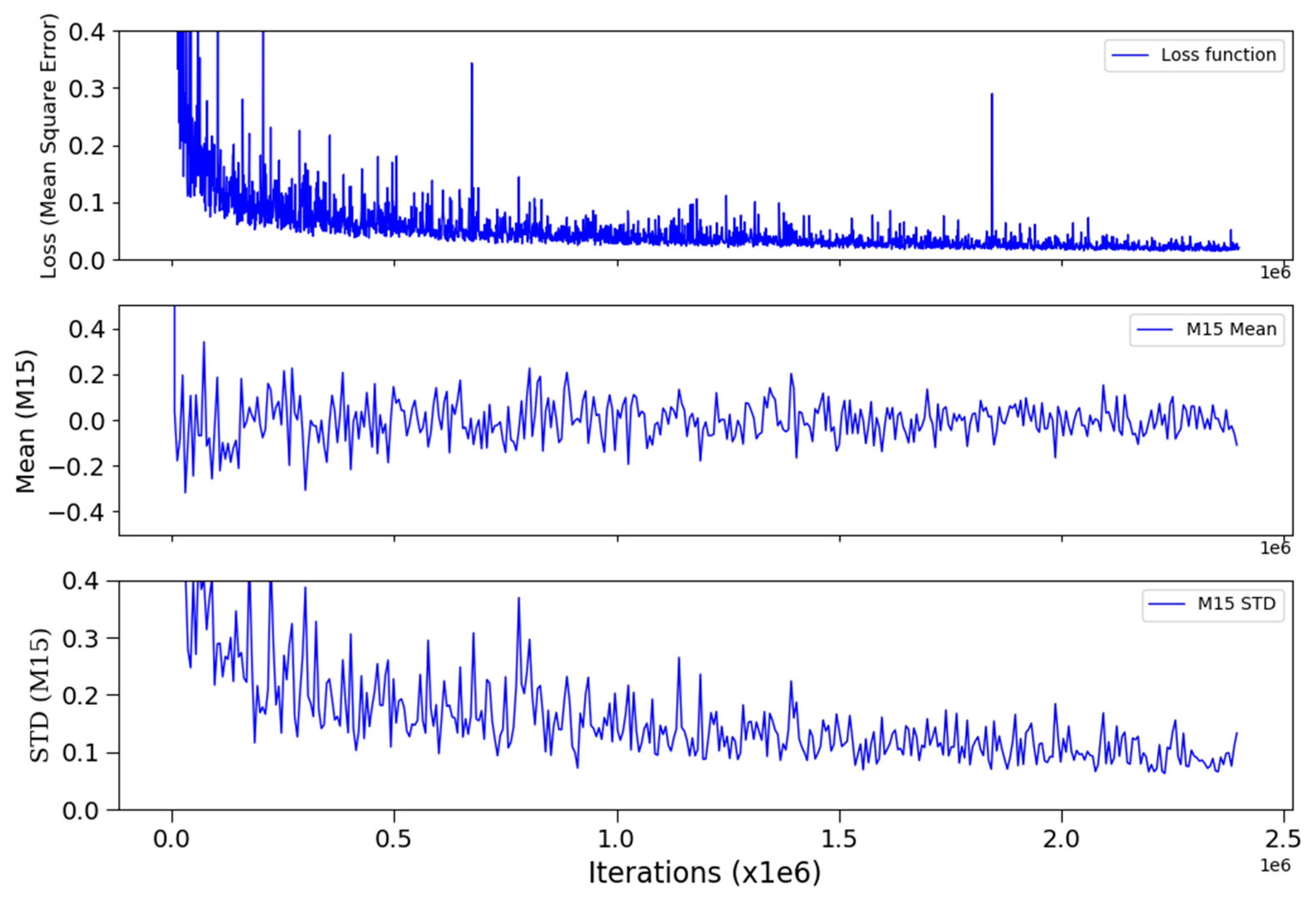
Figure 2 depicts changes in the cost function and the corresponding mean and STD of the testing data for M15 during the training. We recorded the values of the cost function after every 1000 iterations, but we tested the model every 6000 iterations. The value of the cost function began at ~80,000, which is cut from the figure to emphasize the latest convergence. However, it can be estimated by calculating the MSE for the typical BTs of five TEB/M bands. For instance, for a typical BT with 280 K after the first iteration of training, the MSE calculated from the forward propagation should be close to the square of 280, which was close to our expected value. The cost function rapidly reduced from ~80,000 to 0.1 during the first several 10,000 iterations and then gradually became smaller as the iterations increased. During the entire training, the cost function oscillated up and down, but persisted in decreasing, although at increasingly slow speeds, and remained nearly constant at the end of the training. The persistent decreasing of the cost function implies that the BN introduced in the model might mitigate the vanishing gradient problem for a long-iteration training, as the change in the cost function became extremely small in later iterations. In the meantime, the massive amount of input data, which covered all seasons, provided a larger data extent to optimize the model more adequately for a long training time.

Similar to the cost function, the mean and STD were quickly reduced at the beginning of the training and gradually converged as the iterations increased. The mean quickly dropped to its global minimum midway through training, while the STD continued to decrease and was finally stable at the end of the training. We present only the trends for the mean and STD for M15, but the performances of other bands were similar. As discussed in [27], the cost function, mean, and STD oscillated up and down during the training; this was due to using small batch sizes instead of a single sample in each iteration.

Table 3. The F-C mean and STD of the train and test data, and predicted data for 02/21/2020 (F-C: difference between FCDN_CRTM BT and CRTM BT; µ: F-C mean bias; σ: corresponding STD).

	Train Data		Test Data		Prediction Data
	µ	σ	µ	σ	µ	σ
M12	−0.0013	0.0313	−0.0013	0.0320	−0.0011	0.0405
M13	−0.0018	0.0329	−0.0018	0.0336	0.0019	0.0408
M14	0.0	0.0444	0.0	0.0454	0.0009	0.0585
M15	−0.0006	0.0505	−0.0005	0.0516	−0.0002	0.0682
M16	−0.0006	0.0620	−0.0006	0.0633	−0.0058	0.0860

compares the F-C mean biases and STDs between the training, testing, and prediction data. The prediction data are discussed in the next subsection. For all bands, the F-C means and the STDs were within several thousandths of a Kelvin and several hundredths of a Kelvin, respectively, and are comparable between the training and testing data sets, suggesting that no significant overfitting occurred in the model. Finally, including BN and regularization, together with the substantial all-seasons data fed into the model, resulted in a well-trained model and a significant avoidance of the overfitting effect.

3.2. FCDN_CRTM Prediction and Validation with the CRTM

The trained FCDN_CRTM was first used to predict five CRTM BTs for February 21, 2020, which is about one month after the nearest training data. We defined these data as prediction data to distinguish between the training and testing data. As CRTM simulation is quite time consuming, VIIRS data were down sampled by a four-by-four window [12] to speed up CRTM simulation for the model validation. To comprehensively validate the model performance, we did not perform any other quality control for all data, except for the FCDN_CSM clear-sky identification. All ocean clear-sky pixels were selected, including full satellite scan swath and high latitude. As a result, 6.5 million pixels were used for the model validation after the FCDN_CSM clear-sky identification.

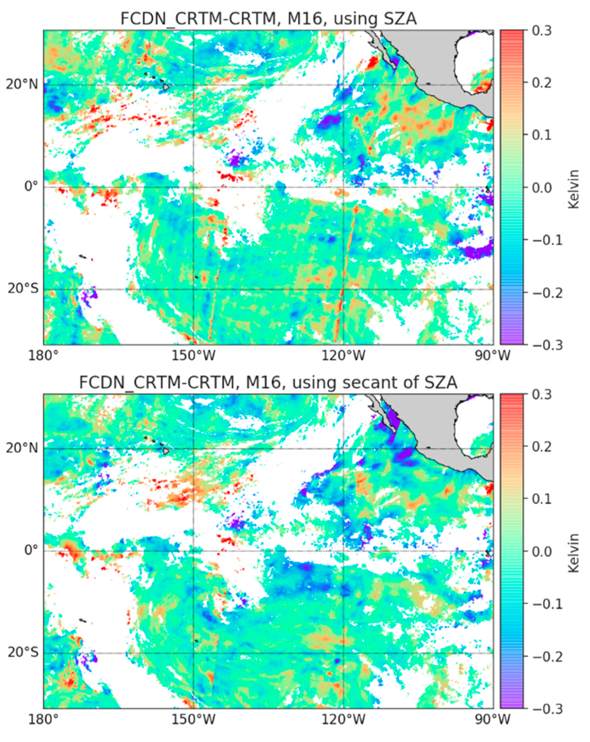
The initial experiment used the direct SZA as an input feature to train the FCDN_CRTM and predict the CSM for 02/21/2020, which was similar to its use in the FCDN_CSM. However, a distinct stratification structure persisted in the global distribution of the F-C, regardless of how we tuned the model. Figure 3 (upper panel) depicts this specific texture in the east Pacific Ocean for the M16 band, which is the most pronounced among the five TEB/M bands. As the forward radiance is more related to the cosine of SZA than the SZA itself, by using a secant of SZA as the input feature instead of SZA in the same training condition, the stratification structure was removed completely in the prediction data, as illustrated in the bottom panel of Figure 3. This slight change to the input feature resulted in a significant improvement in the model, strongly indicating that feature selection is important for the ANN model. Hereafter, the secant of SZA was selected as the input feature in this study.

Figure 4 portrays the global distribution (left panel) and histograms (right panel) of the F-C mean biases in M12, M15, and M16. A summary of the corresponding F-C statistics for all five bands is listed in the right two columns of Table 3. Note that the train and test data sets were generated using the ACSPO CSM as clear-sky identification, whereas the prediction data used the FCDN_CSM, which was trained with the ACSPO CSM. Therefore, in Table 3, the STDs were slightly reduced for prediction data mainly due to possible residual clouds and outliers, rather than significant overfitting existence. This saying was further verified by the later analyses of the long-term stability. Furthermore, the global distributions were generally uniform, particularly for the most atmosphere-transparent band—M12—followed by M15 and M16. The F-C means were Gaussian distributed, and the global means were typically ±0.002 K, with uncertainties of several hundredths of a Kelvin for all five bands. Further analysis showed that the correlation coefficients between FCDN_CRTM prediction and CRTM simulation are typically 0.9999 for all five bands. All statistics analyses indicated that the model is quite accurate for BT prediction with most atmospheric and geographic conditions. In addition, some outliers had slightly larger biases for M15 and M16 in the high SZA, which may be due to the low accuracy related to a long atmosphere path.

Figure 5 further validates the model performance in the SZA and total column water vapor (CWV) content dependencies of the F-C differences. Both parameters are the key factors to evaluate radiative transfer model performance. The left panel shows the SZA dependence of the F-C mean, STD, and corresponding histograms. The right panel is the same as the left, but for CWV. For both SZA and CWV, no significant dependencies of the F-C mean biases were observed. All curves of these F-C biases are within a small amplitude range from −0.05 to 0 for all SZA and CWV bins, which suggests that the FCDN_CRTM can reproduce CRTM BTs accurately for different SZAs and CWVs. In addition, there was slight noise at the high CWV, due to the small data portion in the corresponding bin. Moreover, the uniform distribution performance even existed in the SZA dependencies of the STD (e.f. L2 moment) when the SZA ranged from −55° to 55°. The dependencies gradually increased after an SZA larger than 55°, but the maximum increasing amplitude was still ~0.05 K for M16. The amplitudes of the CWV dependencies were [0.02, 0.08] for M12 and M13, [0.04, 0.09] for M14 and M15, and [0.08, 0.12] for M16. Although the CWV dependencies of the STD were slightly larger than those of the SZA, the amplitudes were still within several hundredths of a Kelvin.

Overall, for all TEB/M bands, the FCDN_CRTM-predicted BTs are generally consistent with the CRTM for different SZAs and CWVs, suggesting that the model is robust for BT prediction under most atmosphere and geographical conditions. However, slightly large STDs were found with a high SZA and a large CWV, particularly for M16, indicating that the FCDN_CRTM can still be fine-tuned to improve accuracy and spatial stability.

3.3. FCDN_CRTM Validation with VIIRS SDR Data

Similar to the CRTM applications, one ultimate goal of the FCDN_CRTM is to evaluate and monitor the accuracy, stability, and cross-sensor consistency of the VIIRS radiometric biases. Hence, FCDN_CRTM model validation with VIIRS SDR data is necessary to check the model performances in extensive atmosphere and geographical conditions. As the VIIRS O-M biases have been successfully used in the past decade to validate CRTM performance under a global ocean clear-sky condition for infrared atmosphere window bands [3,8,9,10], in this section, we use a similar method and focus on the consistency between the VIIRS observation minus FCDN_CRTM prediction (V-F) and the VIIRS minus CRTM simulation (V-C).

Figure 6 presents the global distributions of the V-C (left panel) and V-F (right panel) for M12, M15, and M16, and the corresponding histograms are shown in Figure 7. The global distributions were quite consistent between V-F and V-C, and both mean biases for M12 were only negative several hundredths of a Kelvin. Both V-F and V-C exhibited negative biases in long-window IR (LWIR) bands – M15 and M16 (the root sources of the negative V-C biases for LWIR have been discussed in [3,8], wherein one of the key factor is possible residual clouds). However, the negative mean biases for V-F (−0.02 K, −0.27 K, and −0.35 K for M12, M15, and M16, respectively) were all slightly smaller than for V-F, suggesting that the FCDN_CRTM prediction is closer to VIIRS observations. Additionally, the STDs of 0.32, 0.44, and 0.53 K for V-F are extremely comparable to those for V-C, and the largest difference was only 0.005 K in M16. The summary of global statistics of V-C and V-F, including M13 and M14, are listed in

Table 4. Global mean and STD for SNPP VIIRS on 21 February 2020 between V-C and V-F (V-C: difference between VIIRS BT and CRTM BT; V-F: difference between VIIRS BT and FCDN_CRTM BT; µ: V-C or V-F mean bias; σ: standard deviation).

	V-C		V-F
	µ	σ	µ	Σ
M12	−0.0405	0.3160	−0.0383	0.3185
M13	−0.5894	0.2650	−0.5894	0.2680
M14	−0.5212	0.3850	−0.5168	0.3895
M15	−0.2932	0.4390	−0.2885	0.4440
M16	−0.3811	0.5255	−0.3690	0.5318

, which shows that the means and STDs for M13 and M14 are also similar to those of M12, M15, and M16.

Overall, the global distribution, histograms, and statistics data provide strong evidence that V-F is consistent with V-C under most atmosphere and geographical conditions, and the BTs predicted by the FCDN_CRTM were reasonable and accurate in the global ocean clear-sky domain for VIIRS TEB/M bands.

3.4. Long-Term Stability of the FCDN_CRTM

In this study, the stability of the FCDN_CRTM is not only key to the performance for the long-term monitoring of sensor radiometric biases, but also a way to check whether there is any overfitting in the model. For this purpose, we used the trained model to additionally predict BTs for five dispersion days—03/16/2020, 04/15/2020, 05/16/2020, 06/10/2020, 07/01/2020, and 07/30/2020—where we selected one day in each month from March to July 2020. Including 02/21/2020, seven days’ data were used to evaluate the stability of the FCDN_CRTM. Note that the day selection was random, and as with data from 02/21/2020, we did not perform any quality control for the data, except for the clear-sky identification by the FCDN_CSM.

Figure 8 illustrates the time series of the F-C error bars from M12 to M16 for the seven days. The VIIRS clear-sky pixels were identified by the FCDN_CSM. The blue dashed line represents the mean for all seven-day data and all bands, and together with two blue dashed lines (y = mean-0.1 and y = mean + 0.1), the three dashed lines help to be more intuitive in checking day-to-day changes of the F-C mean and STD. A corresponding comparison between V-C and V-F is presented in Figure 9 for M12, M15, and M16. The F-C mean biases persisted for several thousandths of a Kelvin for all analyzed days and all bands. The average of the F-C means were −0.008, −0.006, −0.008, −0.011, and −0.013 K for M12 to M16, respectively, and the change was not significant over the time period. As expected, the STDs on 02/21/2020, listed in Table 3 were the smallest among the seven days for all bands, as this day is closest to the training data period. However, the STD changes were minimal in the first three days, and the amplitude of the change was between 0.001 K and 0.009 K for all bands. Even on 5/15/2020 and 6/10/2020, the STDs only increased by a maximum 0.039 K in M12 in comparison to the most accurate on 02/21/2020. After 06/10/2020, the STDs significantly worsened, and on 07/30/2020, they were 3–4 times more than on other days. Recall that the regularization and BN were introduced in the model, and all season data were included in model training. All efforts were intended to avoid overfitting of the deep learning model. However, 278 input features and a complicated model architecture may result in overfitting not being fully eliminated. Moreover, the seasonal cycle and extreme climate events [34] could cause possible noise during the model prediction. Interestingly, both means and STDs between V-C and V-F persisted consistently longer in Figure 9, wherein the changes in mean and STD from 02/21/2020 to 07/01/2020 are typically only between 0.01 K and 0.038 K for all bands. Then, the V-F STD increased by ~0.055 K on 07/30/2020. Overall, the stable means and STDs of F-C and the consistency between V-F and V-C from 02/21/2020 to 06/10/2020 provide strong evidence that the robust performance of the FCDN_CRTM can be extended from 5 months to half a year. However, model retraining is needed to maintain a high accuracy of the FCDN_CRTM prediction after that period.

4. Discussion

4.1. Efficiency of FCDN_CRTM

As discussed in the last section, one advantage of the FCDN_CRTM is that the model reproduced similar accurate BTs as CRTM simulation, without using a complicated radiative transfer equation. Furthermore, with the same NOAA STAR Linux server (without GPU support), the CRTM simulation for 6 million clear-sky points required approximately 12 min. In contrast, the total processing time for the FCDN_CRTM with multi CPUs is only 17 s, which was about 42 times faster than the CRTM. On the other hand, even we set one CPU to conduct FCDN_CRTM prediction, which is the same condition with that for CRTM simulation, the total processing time to predict the same amount data is no more than 40 s, suggesting that the high efficiency of FCDN_CRTM is mainly due to its inherent high-efficient calculation, rather than just because it utilizes as many as possible CPU resources. This further implies that the model has a strong capability to efficiently simulate high-resolution spatial and temporal sensors, even for insufficient CPU resources. Certainly, the more data are processed, the more memory is needed.

4.2. End-to-End System

In this study, the whole algorithm included data collection and preprocessing, clear-sky mask prediction, and VIIRS BT prediction and validation. In addition, model training of the FCDN_CSM and FCDN_CRTM was separate from the system. Thus, combining all components, we have built an end-to-end AI framework to predict VIIRS BTs. It first inputs VIIRS SDR, ECMWF data, and CMC SST to the data preprocessing module. This module then collocates atmosphere and surface gridding data in space and time to the VIIRS pixel level and generates both the FCDN_CSM input data with 11 features and the FCDN_CRTM with 278 features. Thereafter, the FCDN_CSM input data are fed into the FCDN_CSM model to produce the VIIRS clear-sky mask. The predicted VIIRS CSM are further input into the clear-sky identification module to identify clear-sky pixels for the FCDN_CRTM input data. Finally, the FCDN_CRTM input data with clear-sky mask are fed into the FCDN_CRTM to predict five TEB/M BTs, and the results are input into the validation module to validate prediction data with CRTM simulation or VIIRS SDR data. The whole system is illustrated in Figure 10.

This framework has the potential to build a system for real-time monitoring of VIIRS BTs against AI predictions. It can input VIIRS SDR data for granules, orbits, or an entire day, in conjunction with the ECMWF and the CMC, to predict corresponding clear-sky BTs and to evaluate VIIRS data simultaneously. As discussed in the previous section, the FCDN_CRTM is much more efficient than CRTM simulation and has a better design for real-time monitoring of VIIRS radiometric biases. Furthermore, the framework makes it easy to extend our research in the future to include land, cloud, and other conditions.

5. Conclusions

An FCDN algorithm, namely, the FCDN_CRTM, was proposed to explore the efficiency and accuracy for reproducing VIIRS BTs in five TEB/M bands. The model was trained and tested in the nighttime global ocean clear-sky domain, in which the CRTM simulation has been well validated in recent years. The ECMWF atmosphere profile and the CMC SST were used as FCDN_CRTM input, and the CRTM BTs were defined as labels.

Efforts were made to improve model performance by iteratively refining the model design and carefully treating the input data. The FCDN_CRTM was designed with three hidden layers, with 512, 384, and 64 neurons in each layer, respectively. We used 278 features as input and five VIIRS TEB/M BTs as output, and the six dispersed days of data from 2019 and 2020, which constituted approximately 40 million samples and covered all seasons, were selected to train the FCDN_CRTM. The trained model was employed to predict CRTM BTs on seven randomly selected days from 21 February to 30 July 2020—nearly one day per month. The predicted BTs were validated with the CRTM BTs and VIIRS SDR data for both accuracy and stability. Moreover, the earlier published FCDN_CSM was used to quickly identify clear-sky pixels for the FCDN_CRTM prediction, and BN, which was introduced in the FCDN_CRTM, sped up the model convergence and further reduced the STD by ~0.2 K. Furthermore, both BN and regularization used in the model, together with the all-season data fed into the model training, aided in avoiding overfitting and made the model more robust. In addition, a secant of the SZA used as FCDN_CRTM input instead of the SZA itself significantly improved the model prediction performance.

Using a line-by-line RTM (LBLRTM) simulated BT as the FCDN model reference could be more reasonable and accurate than CRTM, as the LBLRTM provides spectral radiance calculations with accuracies most consistent with the sensor measurements [35]. However, its computational inefficiency prevents the possibility of large data sample collection for FCDN_CRTM training, testing, prediction, and validation. In contrast, the CRTM’s accuracies have been well validated, although the model is an approximate RTM that uses trained transmittance coefficients. Especially for the TEB bands, the root MSE between the CRTM and the LBLRTM is only ~0.016 K [31], and using CRTM BT as the FCDN_CRTM reference is, thus, adequate for high accuracy and efficiency in this initial study.

As a result, the F-C means were within several thousandths of a Kelvin, and the STDs were within several hundredths of a Kelvin for all bands, and they are comparable between the training and testing data sets. The high accuracies could persist for about half a year before the STDs degrade significantly. In addition, the FCDN_CRTM-predicted BTs are generally consistent with those of the CRTM with different SZAs and CWVs for all TEB/M bands under most atmosphere and geographical conditions. By validation with VIIRS SDR in global distribution and corresponding histograms, V-F was consistent with V-C in most atmosphere and geographical conditions, and the consistencies lasted even longer than the stable F-C period. Furthermore, the FCDN_CRTM processing time was at least one order of magnitude faster than the CRTM simulation. The highly efficient and accurate FCDN_CRTM is, thus, a potential solution to real-time monitoring of global O-M biases for high-resolution VIIRS. We plan to continue to monitor the model’s result periodically under the framework to check for any anomalies and find possible physical explanations. Our future work will extend the FCDN_CRTM functionalities to include land, cloud, and other conditions in the FCDN_CRTM end-to-end framework.