Article

Object-Oriented LULC Classification in Google Earth Engine Combining SNIC, GLCM, and Machine Learning Algorithms

Department of Agricultural, Food, and Environmental Sciences, University of Perugia, 06121 Perugia, Italy
*
Author to whom correspondence should be addressed.
Remote Sens. 2020, 12(22), 3776; https://doi.org/10.3390/rs12223776
Submission received: 12 October 2020 / Revised: 10 November 2020 / Accepted: 13 November 2020 / Published: 17 November 2020
(This article belongs to the Collection Google Earth Engine Applications)

Abstract

:
Google Earth Engine (GEE) is a versatile cloud platform in which pixel-based (PB) and object-oriented (OO) Land Use–Land Cover (LULC) classification approaches can be implemented, thanks to the availability of the many state-of-art functions comprising various Machine Learning (ML) algorithms. OO approaches, including both object segmentation and object textural analysis, are still not common in the GEE environment, probably due to the difficulties existing in concatenating the proper functions, and in tuning the various parameters to overcome the GEE computational limits. In this context, this work is aimed at developing and testing an OO classification approach combining the Simple Non-Iterative Clustering (SNIC) algorithm to identify spatial clusters, the Gray-Level Co-occurrence Matrix (GLCM) to calculate cluster textural indices, and two ML algorithms (Random Forest (RF) or Support Vector Machine (SVM)) to perform the final classification. A Principal Components Analysis (PCA) is applied to the main seven GLCM indices to synthesize in one band the textural information used for the OO classification. The proposed approach is implemented in a user-friendly, freely available GEE code useful to perform the OO classification, tuning various parameters (e.g., choose the input bands, select the classification algorithm, test various segmentation scales) and compare it with a PB approach. The accuracy of OO and PB classifications can be assessed both visually and through two confusion matrices that can be used to calculate the relevant statistics (producer’s, user’s, overall accuracy (OA)). The proposed methodology was broadly tested in a 154 km2 study area, located in the Lake Trasimeno area (central Italy), using Landsat 8 (L8), Sentinel 2 (S2), and PlanetScope (PS) data. The area was selected considering its complex LULC mosaic mainly composed of artificial surfaces, annual and permanent crops, small lakes, and wooded areas. In the study area, the various tests produced interesting results on the different datasets (OA: PB RF (L8 = 72.7%, S2 = 82%, PS = 74.2), PB SVM (L8 = 79.1%, S2 = 80.2%, PS = 74.8%), OO RF (L8 = 64%, S2 = 89.3%, PS = 77.9), OO SVM (L8 = 70.4, S2 = 86.9%, PS = 73.9)). The broad code application demonstrated very good reliability of the whole process, even though the OO classification process resulted, sometimes, too demanding on higher resolution data, considering the available computational GEE resources.

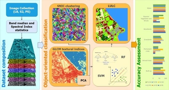
Graphical Abstract

1. Introduction

Satellite remote sensing (RS) provides essential data that helps in mapping and studying the Earth’s surface. RS data archives, thanks to the growing availability of satellites and the increase of image resolutions (radiometric, spectral, spatial, and temporal) are constantly expanding, allowing the users to potentially access and analyze very large time-series datasets, but at increasing time and computational costs. In the last decade, RS data processing has moved from traditional workstations equipped with state-of-the-art (and often very expensive) hardware, and RS software, to cloud-based platforms that allow users to instantly access and analyze huge pre-processed geospatial data through user-friendly, web-based interfaces, and effective scripting languages. Among these platforms, Google Earth Engine (GEE) is achieving considerable success because it is a cloud-based geospatial analysis platform that allows users to solve, in a very efficient way, the primary problems related to the management of immensely large amounts of data, their storage, integration, processing, and analysis [1].
A typical RS data application is the production of Land Use/Land Cover (LULC) maps, which describe how land is used for various human purposes, such as agriculture or residential areas, or the physical characteristics of the Earth’s surface (i.e., water bodies, grasslands, rocks) [2]. LULC maps are very useful for analyzing landscape composition and configuration, and for detecting changes that are taking place in the landscape, as well as considering transformations with environment gradients [3,4]. Understanding the LULC changes and spatially identifying the transformation hotspots are extremely relevant for ecosystem monitoring, planning, and management. Such classifications generally require an initial step aimed at the multitemporal image composition to limit the cloud coverage and to calculate image statistics and spectral indices used to improve the classification accuracy. In this regard, GEE allows the users to define different modus operandi for the combination of the input data, allowing to efficiently create light, cloud-free, multi-temporal, composite dataset without having to run into blocks related to limited local computational resources images [5,6].
Ordinary LULC automatic classification approaches, applied to RS data, are based on a calculation of spectral signatures of selected LULC classes using training data and pixel-based discrimination between different land cover types [7]. Thanks to the recent improvements in image segmentation algorithms, the object-based approaches (so-called Geographic Object-Based Image Analysis—GEOBIA) are becoming more popular compared to traditional image analysis and classification, due to their capability in delineating and classifying the landscape objects or patches, at different scales [8]. Object-oriented (OO) methods generally produce better results on higher resolution data, despite the higher computational costs of segmentation and the use of several features for the classification, while the use of the pixel-based (PB) approach is typically recommended for lower resolutions. The latter, as frequently happens, suffers from the so-called “salt-pepper” effect on higher spatial resolutions. The object delineation is performed in a crucial step based on an image clustering and segmentation aimed at grouping similar pixels into image clusters and converting them to vectors [9,10,11]. In this regard, the Simple Non-Iterative Clustering (SNIC) algorithm, available in GEE, resulted very efficient in grouping similar pixels and identifying potential, individual objects [12]. After the segmentation, GEOBIA generally combines spectral and spatial information with the texture and context information of the image to perform the final object classification [13]. In GEE, the Gray-Level Co-occurrence Matrix (GLCM) is available, a very effective method for the extraction of 18 textural indices from 8-bit greyscale images. This feature appears very useful since allowing the GEOBIA application even on greyscale images. The subsequent application of the Principal Component Analysis can help in effectively reducing the high dimensionality of GLCM outputs in a few, representative bands [14].
The classification step, both in PB and OO processes, can be performed using various solutions. The recent Machine Learning (ML) classifiers have demonstrated a higher performance compared to the traditional maximum likelihood ones [15] and do not require any assumptions about the data distribution. In particular, non-parametric ML classifiers, such as Classification and Regression Trees (CART), Random Forest (RF), and Support Vector Machine (SVM) have been reported to provide extremely accurate LULC classification results from remotely sensed images [16,17]. CART is a simple binary decision tree classifier and works using a pre-defined threshold [18], while RF is an ensemble classifier based on the combination of multiple CART-like trees. RF is highly efficient and accurate, and is one of the favorite classifier for LULC classification [19,20], because, generally, it performs better than other popular classifiers [21]. SVM is a well-performing classifier, but appears slightly more complex since it requires the choice and tuning of kernels and other input parameters [22,23]. Most of these classification methods rely on high-quality training data, and on proper combinations of features that directly affect the stability of the classification results [24]. The selection and implementation of such features are generally time-consuming and require wide engineering skill and technical expertise. Differently, in modern Deep Learning (DL) approaches, features are automatically implemented from input data using learning procedures based on neural networks that generate multiple processing layers. These layers provide more effective feature representations through multiple abstraction levels which result very effective in discovering complex structures and discriminative information hidden in multi-dimensional data [25]. DL models can be also used in GEE through the TensorFlow platform [26]; however, their implementation is not straightforward for ordinary GEE users, since these models must be developed and trained outside GEE using the GEE API and the Google Colab platform. Thus, the application of ordinary ML classification algorithms, such as RF and SVM, is still a convenient option in the GEE environment.
GEOBIA, including both object segmentation and object textural analysis, is still no common in the GEE environment, probably due to the difficulties existing in concatenating the proper functions and in tuning the various parameters to overcome the GEE computational limits. The SNIC algorithm has been widely used in GEE to identify spatial clusters and improve LULC classification. For instance, Mahdianpari et al. [27,28], to produce the Canadian Wetland Inventory, implemented an object-based classification of S2 and S1 data, based on SNIC and RF, which substantially improved the PB classification. Paludo et al. [29] mapped soybeans and corn in Paraná, achieving very high accuracy, applying SNIC and the Continuous Naive Bayes classifier on Landsat-8, Sentinel-2, and SRTM+ (Shuttle Radar Topography Mission) data. To classify the LULC of Iran, SNIC was to identify segments on S2 data and to enhance the classification result of the pixel-based RF algorithm using a majority calculation within each segment [30]. Djerriri et al. [31] proposed an object-oriented approach based on the classification of S2 images using SNIC clustering combined with the RF classifier and the results were more accurate than those from the pixel-based approach. Firigato [32] performed an RF classification of high-resolution satellite images using SNIC and subsequent vectorization, and a feature selection based on NDVI mean the gradient of directions, and other properties, such as area, height, and width. In some GEE-based researches, the segmentation step was developed outside GEE. For example, Stromann et al. [33] developed an object-based LULC SVM classification, using S1 and S2 data, through a preliminary segmentation step performed in commercial software and a subsequent feature characterization in GEE based on GLCM. Xiong et al. [34] produced a 30-m cropland map of continental Africa by integrating PB and OO algorithms using S2 and L8 data, using SVM and RF; the segmentation step was based on a recursive hierarchical segmentation carried out on NASA Pleiades supercomputer. The GLCM has been used in GEE to derive textural indices and improve LULC classification. For instance, besides the above-cited research from Stromann et al. [33], Godinho et al. [35] combined multispectral bands with the vegetation indices, and GLCM textures to improve the LULC classification. Mananze et al. [36] derived a Land Cover map of a study area in Mozambique from Landsat 7 and Landsat 8 bands, vegetation indices, and textural features extracted by GLCM. Radar and optical imagery were combined to map oil palm plantations in Sumatra, Indonesia, using GLCM textural features, derived from SAR (Synthetic Aperture Radar) data, to improve the classification [37].
The users of LULC maps need to know how accurate the maps are to use the data more coherently [38]. The most widely used classification accuracy assessment approach is in the form of a confusion matrix based on a comparison between the classification outputs and ground truth data [39,40]. The matrix is used to derive a series of descriptive and analytical statistics (user’s, producer’s, and overall accuracy—OA—and Kappa statistic—K) useful to interpret and synthesize the accuracy level of a given LULC map [16,41]. Despite its broad application, kappa statistics can be very misleading to assess or communicate the accuracy of classification due to its high dependency on the variation of class prevalence [42]. An automatic comparison between PB and OO methods in LULC classification, based on confusion matrices, could result very useful to define the best approach in terms of accuracy of the various LULC classes [43] and to assess the improvement achieved with the OO approach, since the final accuracy is always conditioned by the proprieties of the input data [44], the quality of training information, and the peculiarities of the study areas.
In this context, this work is aimed at developing and testing an OO classification approach combining the SNIC algorithm to identify spatial clusters, the GLCM to calculate cluster textural indices and two broadly used ML algorithms (RF and SVM) to perform the final classification. The proposed approach is implemented in a user-friendly, freely available GEE code useful to perform the OO classification tuning various parameters (e.g., choose the input bands, select the classification algorithm RF or SVM, test various segmentation scales) and compare it with a PB approach. The accuracy of the two approaches is assessed both visually, and through two confusion matrices and their related statistics (producer’s, user’s, and overall accuracy).

2. Materials and Methods

2.1. Study Area

The 154 km2 study area, selected for the development and testing of the proposed methodology, is located around the Trasimeno Lake, in Umbria, Central Italy (43°06′N, 12°07′E) (Figure 1). Lake Trasimeno, the fourth largest Italian lake, is situated in the northwestern part of Umbria and has a surface area of about 120.73 km2 [45]. Since March 1995, the area has become a regional nature park [46]. The lacustrine ecosystem is an area of exceptional value for its wealth of flora and fauna and its diversity of species. Tourism, agriculture, and livestock breeding are the most important activities in the Trasimeno area: cultivated lands cover about 70% of the catchment area of the lake, even if intensive agriculture with irrigational needs is only present in 28% of the area [47]. The zone is characterized by a multifunctional landscape mosaic with high abundance and diversity of agricultural lands (e.g., sow-lands, grasslands, vineyards, olive groves), wooded areas, artificial surfaces, and many small private artificial lakes.

2.2. Training and Validation Sample Data

The study area is featured by a complex landscape mosaic composed of six LULC classes: (1) built-up areas, including settlements and other artificial surfaces; (2) annual crops, comprising various crops such as cereals, grain legumes, and horticultural plants; (3) permanent crops, mainly including vineyards and olive groves; (4) grasslands; woodlands, composed by small and fragmented areas; (5) riparian vegetation and shrubs, including the lakeside or riverside vegetation and other sparse small areas covered by shrubs; (6) water bodies that include the Trasimeno Lake and other small private lakes. To test the usability and reliability of the whole procedure, only 10 points for each class have been identified through the GEE interface, using the S2 RGB and composite infrared layers, and the high-resolution layer of Google Maps, for collecting the training information. A total of 450 validation points were randomly generated and manually labeled through a visual interpretation of the same base layers (Table 1). This approach is largely used in the literature [48,49].

2.3. Methodology

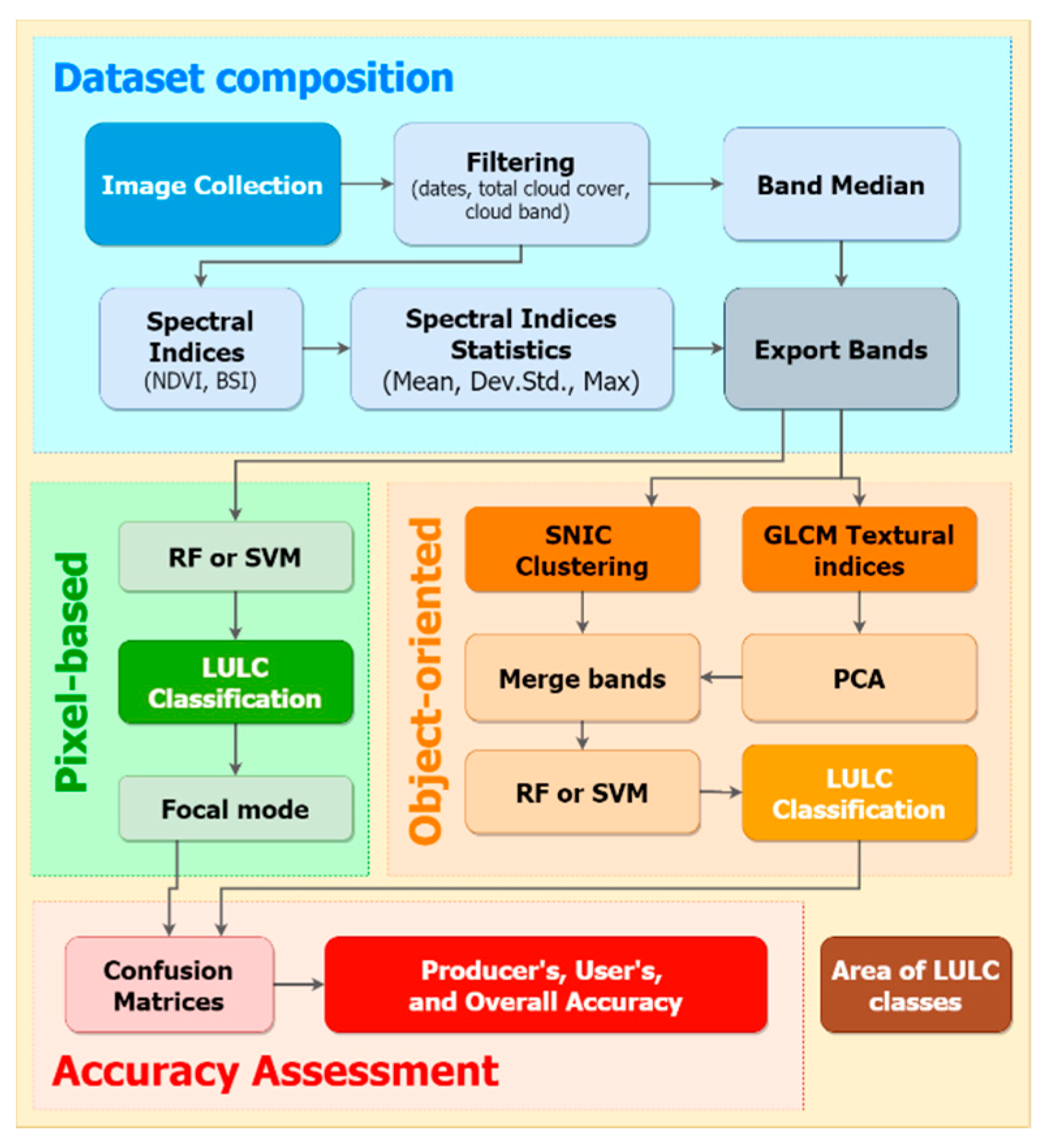
The general workflow is composed of three main steps, implemented in two GEE scripts (Figure 2): the composition of the initial dataset, the LULC classification, and the accuracy assessment. The first step was implemented in a separate script to speed-up the classification and accuracy assessment procedures also considering that the base composite image, once generated, requires fewer adjustments compared to the subsequent steps. The classification and accuracy assessment steps were implemented in a single GEE script. The former includes a PB and an OO approach, both using the same training data and applying the RF or the SVM classifier. The latter was performed, for both methods, through a confusion matrix using the same, above-mentioned, validation data.
To investigate the reliability of the proposed approach, verify its applicability on different resolution RS data, and assess the influence of some important input parameters, the code was broadly tested on the study area: (a) using data from three different satellites—Landsat 8 (L8), Sentinel 2 (S2), and PlanetScope (PS); (b) applying the RF or the SVM classifier; (c) including or excluding textural information for the OO approach; (d) using different seed distances for spatial cluster identification. PlanetScope images were chosen to test the code on higher spatial resolution data considering that, in GEE, S2 is the highest spatial resolution data available for the study area.
The results were preliminarily compared in terms of overall accuracy. On this basis, the most effective OO and PB parameter combinations were selected for each dataset and compared both visually and in terms of percentage of total area, user’s and producer’s accuracy of LULC classes. The execution time of the selected classification was measured and compared as well.

2.3.1. Dataset Composition

The creation of the base dataset is generally a critical step for every LULC classification. In this application, the composition of this dataset for the L8 and S2 data starts, in GEE, from a filtered and cloud-masked image collection. Then, the Normalized Difference Vegetation Index (NDVI) and the Bare Soil Index (BSI) are calculated for each image. The NDVI is often used for the mapping of changes in land cover [50,51] and, according to Singh et al. [52], this index, used in the LULC classification, produces a significant improvement in classification accuracy. The BSI is mainly used to highlight the difference between agricultural and non-agricultural land thanks to its enhanced ability in identifying bare soil and fallow lands [53]. These additional indices are commonly used to improve the LULC classification. Data augmentation was implemented using the main statistics of NDVI and BSI (mean, standard deviation, and maximum) to generate six additional bands containing main statistics of the two spectral indices useful to account for season variability of the LULC classes. The code generates a final composite dataset calculating the median pixel values for the selected bands and adding to the composite the selected spectral indices statistics among those available. The final phase is the export of the desired bands of the dataset.
The input requirements to set for the execution of the code are:
  • roi (region of interest), a polygon used to delimitate the study area;
  • period of interest, based on the definition of start date (MM-DD-YYYY) and end date (MM’-DD’-YYYY’);
  • inBands, which are the input bands selected from the L8 or S2 available bands [45];
  • outBands, which are the output bands of the final dataset. As Indicated, they are selected from the median of the inBands and on the other mean, max, and standard deviation of NDVI ad BSI indices.
In detail, the code performs an initial collection of images filtered by the specific period of interest (three years, from 1 January 2017 and 31 December 2019), the region of interest (roi), the maximum percent of cloud cover (10), and the cloud mask (maskS2clouds). The cloud cover masking for S2 is computed using the QA60 band provided in GEE with the S2 Surface Reflectance data. QA60 band is a 60 m resolution layer that combines dense clouds and cirrus clouds mask [54]. The cloud cover masking for L8 is performed using the “pixel_qa” band provided in GEE with the L8 Surface Reflectance data. This cloud-masking step is coherent with Nyland et al. [55] and Xye et al. [56] who suggest selecting input images with a maximum cloud cover and over three years to create a very effective composite image. This selection process produced, for the study area, two image collections, including 43 images for the L8, and 119 images for the S2 on which the “inBands” are selected and the median bands are computed. NDVI and BSI are calculated for each image and the relative spectral indices statistics are obtained using the proper reducer functions. The final exporting phase regards only the desired bands (”outBands”) previously defined. In this application, to create the initial S2 dataset, bands 2, 3, 4, 6, 8, NDVI mean, NDVI Std. Dev. (Standard Deviation), and BSI mean were selected. For composing the initial L8 dataset, bands 2, 3, 4, 5, 6, 7, NDVI mean, NDVI Std. Dev., and BSI means were selected. Differently than L8 and S2, the base dataset for PS data was generated through a simplified composition step, calculating on a pixel-basis the median between the 4 multispectral bands of two images (30 March 2019 and 26 August 2020) collected during the research and uploaded to the GEE cloud. In this case, to account for seasonality, two NDVI additional bands, derived from the two images, were added to the initial dataset.

2.3.2. LULC Classification

The LULC classification is based on a supervised approach which, as usual, needs to collect from the training points the necessary information utilized to train the classifiers [57]. Considering the specific objective of this research, two approaches (PB and OO) were implemented in GEE, both using alternatively the RF or the SVM classifiers. To perform the LULC classification, the code needs this set of inputs:
  • roi: region of interest;
  • newfc: a collection of features containing all training data labeled with codes corresponding to LULC classes;
  • valpnts: validation points randomly generated and manually labeled with the same LULC code used to assess the model’s accuracy;
  • dataset: previously generated in the “Dataset composition” step.
Training data (points or polygons) can be conveniently input using the GEE interface and adding as many feature collections (including more geometries) as the desired LULC classes. To improve the amount of supervised information, a buffer with a fixed radius (10 m) is created around each point. The training information from the “LULC” property of the “Newfc” feature collection is used to train the chosen classifier. The dataset containing the validation points can be inserted using the GEE interface or built-in a GIS environment (e.g., QGIS [58]) and imported in shapefile format. This dataset, as indicated, is used for the accuracy assessments of the two methods.
The code executes the PA and OO LULC classifications according to the two mentioned approaches. In both cases, the classification relies on the same, previously created, initial composite dataset, and training data.
In the PB classification stage, the image is quickly classified by a preliminary definition of the RF classifier, or the SVM classifier, and the subsequent training phase. As generally performed, a band normalization of the input dataset was applied before applying the SVM classification. For the RF classifier, the number of trees was set to 50, while for the SVM a radial basis function kernel (RBF) was applied (with gamma = 1 and cost = 10). To clean up all the output and reduce the “salt and pepper” effect, a final morphological operation (based on a focal mode) is performed on the output classification.
The OO classification stage combines a spatial clustering step, aimed at grouping similar and contiguous pixels together, a subsequent calculation of textural indices on a cluster basis, and a final classification step. In this regard, the proposed method is based on a novel two-step procedure combining the SNIC and the GLCM algorithms, already applied separately in GEE. SNIC is performed on the same bands used for the PB classification, using a regular grid of seeds as input generated by the “Image.Segmentation.seedGrid” function which requires a superpixel seed location spacing (in pixels). The latter influences the cluster size and can be varied to find an optimal value. In the code testing phase, various seed spacing (5, 10, 15, 20 for L8 and S2, and 35, 40, 45, 50 for PS) were applied on the different datasets and compared in terms of OA. These values were identified after some initial general testing and considering the textural characteristics of the landscape patches in the study areas. SNIC identifies the objects (clusters) according to the input parameters and generates a multi-band raster, including the clusters and additional layers containing the average values of the input features. SNIC, in GEE, requires setting some main parameters: the “compactness factor” influences the cluster shape (larger values produce more compact clusters); the “connectivity” (4 or 8) defines if consider a Rook’s or Queen’s contiguity to merge adjacent clusters; a “neighborhoodSize” to avoid tile boundary artifacts. In our application, always considering the study area characteristics, these parameters were set as follows: compactness = 0, connectivity = 8, and neighborhood size = 256. SNIC outputs are variable depending on the visualization scale. Thus, in the code, was necessary to fix a proper output scale of clusters through the “reproject” function (L8 = 30, S2 = 10, PS = 6). For the L8 and S2 the native resolution was used, while, for the PS output, half spatial resolution was chosen to speed up the subsequent steps.
GLCM algorithm, as indicated, requires a grey-level 8-bit image as input. In our code, this image was generated through a linear combination of NIR, Red, and Green bands of the initial composite image, according to the following formula:
Gray = (0.3 × NIR) + (0.59 × RED) + (0.11 × GREEN)
Then, after a proper standardization, a PCA of the most relevant 7 GLCM metric (Table 2), selected according to Hall-Beyer et al. [14], is applied to derive a single representative band (the first PC) which generally contains the vast majority of the textural information. The average of PC1 is then calculated in a separate band for each object included in the SNIC “clusters” band. The PC1 object-averaged band is finally added to those extracted from the SNIC segmentation process. On this dataset, the same definition and training procedure of the pixel-based RF or SVM classification is reproduced to get the LULC classification through the OO approach. To overcome the GEE computational limitations, faced working with PS data, it was necessary to export the final classification to an asset before visualizing the final OO LULC classification. The initial testing on PS data was conducted on a smaller window within the study area.
A final computation is done counting the number of the pixel belonging to each class to calculate the total area (km2 and percentage) for each LULC class. All of these operations are developed in the raster domain to speed up the code execution without applying conversions to the vector domain.

2.3.3. Accuracy Assessment

The accuracy of both LULC classifications is evaluated using a confusion matrix implemented in GEE in which the LULC linked to the validation points is statistically compared with the output classifications. The confusion matrix allows calculating the overall accuracy (OA) and kappa statistics (K) and shows where the classification generates confusion (omission and commission errors, quantified respectively by the user’s accuracy—UA and producer’s accuracy—PA) among the LULC classes producing inaccuracies. The accuracy is typically considered as the degree of closeness of the results to values accepted as true [59], while the Kappa coefficient expresses the proportional reduction of the errors generated by a classification process compared with the error of a completely random classification [60]. In this study, considering the above-mentioned issues regarding the Kappa coefficient [42], only the OA, PA, and UA, derived from the confusion matrices, were analyzed. Of course, many factors can influence the measurement of accuracies, such as the characteristics and the resolution of the satellite data, the distribution of the validation points, and the classes chosen for the LULC classification. In the code, the same steps were applied to assess and compare all the classifications.

3. Results

The OA results from the various tests conducted in the study area are reported in Table 3. The best OA (89.3%) is achieved with the S2 data using the OO method and including the GLCM textural information. On L8 data the PB approach performs better than the OB approach (79.1% vs. 78.4%), while, on the higher spatial resolution datasets, the OO method produces better results (S2: 89.3% vs. 82%; PS: 77.9% vs. 74.8%). The incorporation of the textural information improves the OO classification for both S2 and PS data, even though the increase in OA is more pronounced for the PS dataset (S2: 89.3% vs. 86.6%; PS: 77.9% vs. 74%). The SVM classifier results more effective in terms of OA in both the PB and OO approaches on the lower resolution L8 data (PB: 79.1% vs. 72.7%; OO without GLCM: 78.4% vs. 68%). This classifier performs slightly better with the PB approach on PS data as well (74.8% vs. 74.2%). However, the RF classifier gained better results on S2 data, both with the PB and OO approach (PB: 82% vs. 80.2%; OO with GLCM: 89.3% vs. 86.9%) and with the OO approach on the PS data (77.9% vs. 73.9%).
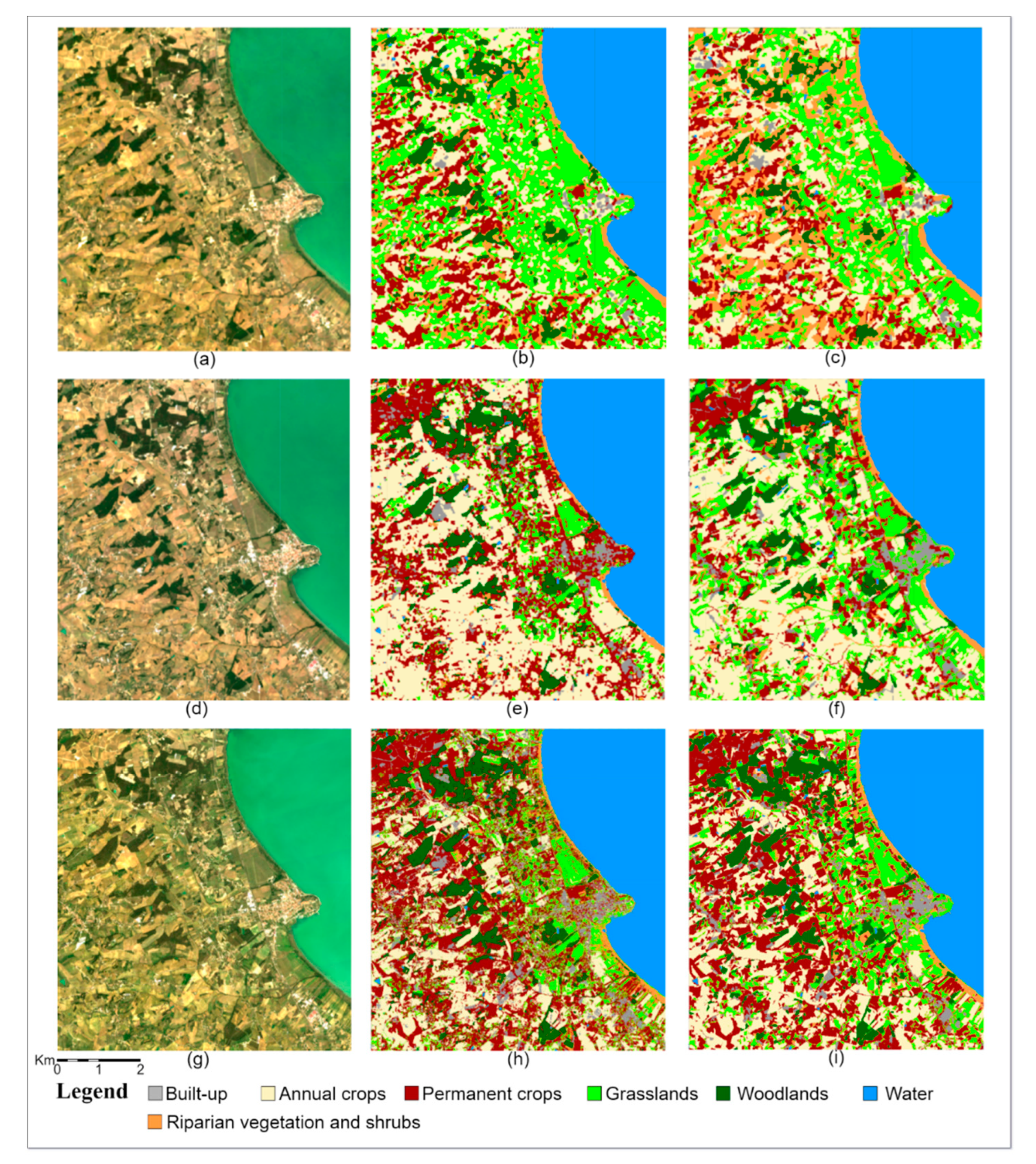
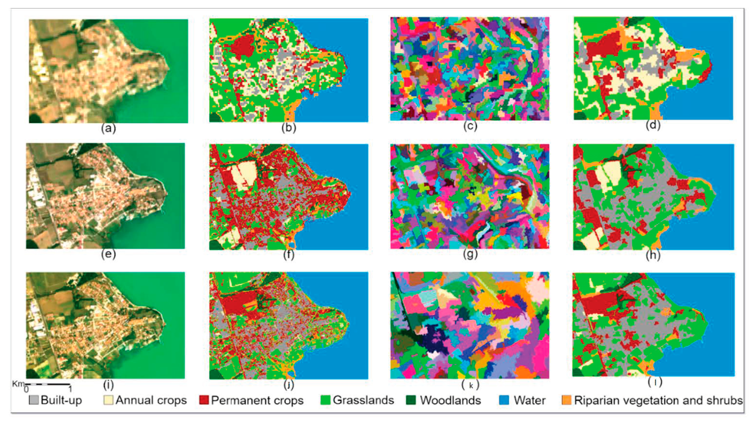
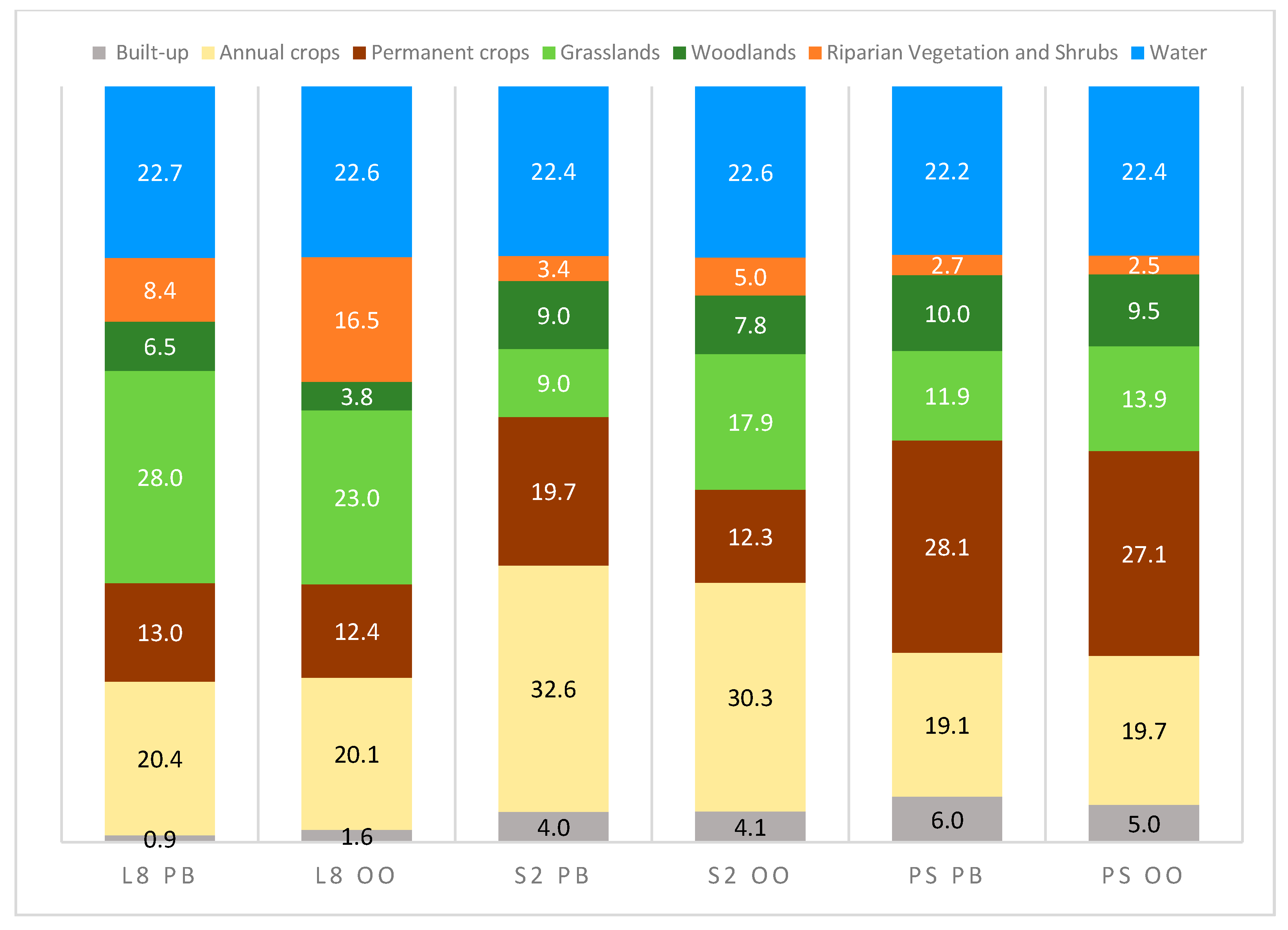
Figure 3 shows the best PB and OO outputs for each sensor selected considering the above-described OA outputs. In Figure 4, the difference between the selected classifications, also in terms of cluster size, is shown in an interesting portion of the study-area characterized by the presence of the main urban center, a section of Trasimeno Lake, and the neighboring multicultural area. The percentage of the total area occupied by each class, according to the selected classification approaches, is reported in Figure 5.
The LULC maps and the related areas of LULC classes show very significant differences between the outputs from the various classification approaches. The main discrepancies, compared to the S2 OO classification, can be observed for permanent crops, grasslands, and annual crops, but, considering their small area coverage, a relevant divergence can be also observed for the built-up areas, and the riparian vegetation and shrubs as well. Built-up areas result particularly underestimated in the L8 classification. Water, woodlands, apart from the L8 classifications, appear more similar in their total extension. However, comparing the LULC maps with the OO S2 output (Figure 3), a very inconsistent spatial configuration of permanent crops, grasslands, and riparian vegetation and shrubs can be observed in the L8 outputs. Similarly, a very abnormal distribution of permanent crops can be observed in the PB S2 and PB PS outputs as well.
A deeper insight into the reliability of the selected outputs and the affordability of the various selected approaches is provided by the comparison of PA and UA derived from the confusion matrices (Figure 6; the full confusion matrices are reported in the Supplementary Materials, Tables S1–S3). PA, quantifying the percentage of correctly classified validation points for each LULC class, supports the interpretation of the omission (or the exclusion) errors (Figure 6a), while the UA, measuring the percentage of correctly classified points in the output LULC classes, indicates the commission (or the inclusion) errors (Figure 6b). As expected, all of the tested approaches perform very well on water and woodlands classes (only L8 OO shows 42% of omission errors of woodlands validation points). Thus, to improve the readability of graphs and to focus on the most interesting results, these classes were excluded from Figure 6 and the following analysis. The other LULC classes are characterized by very variable classification outputs from the different methods. As already shown by the OA, the S2 OO produces the best compromise in all classes in terms of PA and UA. S2 PB shows worse results mainly in the classification of riparian vegetation and shrubs, permanent crops, and built-up areas, while grasslands are classified slightly better than the OO method. Permanent crops, and riparian vegetation and shrubs, as expected considering the S2 resolution, are the most critical LULC classes for both approaches. The inaccuracy of the formers is mainly due to the commission with annual crops and grassland, while the latter is often mixed up with grasslands and woodlands. The accuracy results for the other LULC classes (annual crops, grasslands, woodlands, and water bodies) indicate only small differences between the two approaches from the user perspective.
L8, due to the lower spatial resolution, performs generally worse than S2. Only some classes show a very good PA (grasslands and riparian vegetation and shrubs, especially with the PB approach), but their outputs in the maps are considerably mixed with other classes. Built-up areas from PB show very low inclusion errors, but very high exclusion errors. PA and UA results for PS, despite the higher spatial resolution, show various inaccuracies. The PS OO approach performs generally better than the PB from both the producer’s and the user’s point of view. The most problematic classes are, once again, permanent crops, grasslands, and built-up areas. Despite the low omission errors of the permanent crops and built-up areas, they are characterized by high commission errors in both approaches mainly due to the poor classification of the annual crops (built-up areas have lower commission errors in the OO approach). The annual crops, and the riparian vegetation and shrubs classes, despite the average PA, show a very good UA in the OO approach.
Regarding the execution time of the six selected above-described approaches, as expected, it is proportional to the image resolution and the complexity of the processing. Thus, the OO approach, on average, is more time demanding than the PB one (L8: 15.76 s vs. 6.35 s; S2: 35.75 s vs. 4.11 s; PS: 75.25 s vs. 7.25 s). The PS OO execution time includes the necessary exporting step of the final LULC classification.

4. Discussion

The world of remote sensing (RS) is constantly growing thanks to the launch of new earth observation satellites, to the increasing resolutions of sensors, to the massive archives of (often freely) available data, and to the increased computational resources. Google Earth Engine (GEE) has achieved considerable success because it is a free cloud-based geospatial analysis and modeling platform that allows users to access, observe, and analyze geospatial data over the entire planet, thanks to a huge, ready-to-use data archive that allows the experimentation of many applications. The use of ML algorithms combined with geographic object-oriented analysis (GEOBIA) techniques is constantly evolving, and GEE, as shown in this research, is an effective environment to build multi-temporal composite images, and implement, in a straightforward way, complex image processing and classification processes.
This work successfully developed an object-based approach combining SNIC, GLCM, and ML algorithms in a user-friendly, freely accessible, GEE code. This latter, broadly commented, allows the user to set and tune various input parameters and to compare the results from the OO approach with a PB one, developed with the same input bands and classification algorithm. The comparison can be performed both visually, assessing the output LULC maps, and analyzing the accuracy matrices for a given study area. The matrices allow the user to calculate the user’s and producer’s accuracy for each class and the overall accuracy. These measures give more sound information about the reliability of the two classification approaches and on the possible added value of using an OO approach. In most cases, as highlighted in the introduction, the latter provides higher accuracy in the classification compared to the pixel-based one, due to the combined use of spectral, spatial, and textural information. However, as shown in this study for the L8 data and other researches [44,47], the results are variable depending on the input datasets, the selected LULC classes, and the peculiarities of the study area. In this regard, as shown in this application, the script could be conveniently used to compare the OO and PB results produced using datasets at different resolutions, to test several settings and input parameters, and to select various classification algorithms.
The SNIC resulted very effectively in the object delineation (in this case, the landscape patches), even though, in its ordinary application within GEE, it is based on a regularly spaced grid of seeds. In this regard, a possible improvement could be the use of seeds generated identifying the local minimum or maximum of variance [61]. As shown in this application, testing the outputs of various seed spacing could be very useful in finding the more effective cluster size also considering the size of the landscape patches. Compared to previous studies, the proposed approach combined SNIC with GLCM to analyze the textural features of the input datasets. This is a widely used algorithm in image-processing which has shown, also in GEE, a very good performance in characterizing the objects’ textures through a wide range of textural indices. In the code, a subsequent application of a PCA on the seven most important GLCM metrics allows the user to include in the OO classification a single band that synthesizes the majority of the available textural information. If necessary, considering the relative variance expressed by the PCs calculated by the code, more PCs could be selected and used for the classification. This step resulted very useful since it relieves the user from the selection of the more effective GLCM metrics to be used in the classification.
As indicated, all of the object identification and subsequent textural characterization were developed in the raster domain on which GEE performs very well. Such an approach, even though associated with quicker code execution, does not allow considering the object size and shape, which could be very important for regular objects at higher resolutions. The vectorization of objects could overcome this limitation, as proposed by Firigato [32], however, considering the raster oriented GEE environment, the few attempts in this direction are characterized by a very slow code execution or by a block in processing due to a too large number of geometries.
GLCM information, even with the 10 m S2 resolution, improved both the classification of very heterogeneous and complex LULC classes, such as the built-up areas (due to their high internal entropy [62]) and the identification of those patches characterized by a regular texture, such as the permanent crops. This LULC class, including mainly olive- and vine-yards with a tree spacing lower than the S2 (and even than the PS resolution), was included as a challenge to explore the OO potentiality in GEE. The very good accuracy obtained for this class, together with that achieved for the built-up areas, clearly demonstrated a great potentiality of the proposed OO methodology even with S2 data. Differently, the application of this method on L8 data, using SNIC, or SNIC and GLCM did not improve the PB output. This is probably due to the impossibility with the L8 spatial resolution of reading relevant textures of landscape patches within the study area. Unexpectedly, the PlanetScope dataset, despite its more than triple spatial resolution, produced inferior overall results compared to S2, even adopting an OO approach. This result is probably related to the lower temporal and spectral resolution of this dataset, and to the rather few training points used which, together, provided scarce information to properly differentiate the various agricultural classes. Therefore, even though the permanent crops are well recognized both in the PB and OO approach (with a similar UA of the S2 OO), the poor classification of annual crops and grasslands generated a considerable commission in all the three agricultural classes. This may suggest that the 3 m spatial resolution did not provide enough textural information for effective separation of the three agricultural classes and that the S2 higher temporal and spectral resolution, summarized by the median bands and the spectral index statistics resulted, in this regard, more effective. Using a timely more extended initial PS dataset could help in improving the LULC accuracy produced using this data source.

5. Conclusions

GEE showed, once again, considerable versatility and adaptability due to its cloud architecture, its user-friendly interface, and its efficient scripting language. Within the GEE environment, this work developed and tested an OO classification approach combining the SNIC algorithm to identify spatial clusters, the GLCM to calculate cluster textural indices and two broadly used ML algorithms (RF and SVM) to perform the final classification. The approach was implemented in a user-friendly code useful to compare the OO and PB classification approaches, tuning various settings and input parameters. In the study area, the OO approach produced a sensible accuracy improvement for S2 and the PS datasets. Despite the lower spatial resolution, S2 achieved better results than PS thanks to the higher temporal and spectral resolution. Due to the lower spatial resolution and considering the study area features, the OO method did not produce better results than the PB approach on L8 data. Our application demonstrated the reliability of the whole methodology, even though the OO classification, due to its higher complexity, results more computationally demanding, and tends to slow down (and sometimes block) the GEE code execution, especially using higher-resolution data.

Supplementary Materials

The following are available online at https://www.mdpi.com/2072-4292/12/22/3776/s1, Table S1: PB and OO confusion matrices for L8, Table S2: PB and OO confusion matrices for S2, Table S3: PB and OO confusion matrices for PS. The GEE codes processing S2 data, developed in this research, are freely available on line at https://code.earthengine.google.com/?accept_repo=users/mvizzari/Tassi_Vizzari_RS2020.

Author Contributions

Conceptualization, M.V. and A.T.; methodology, M.V. and A.T.; software, A.T.; original draft preparation, A.T.; writing—review and editing, M.V. All authors have read and agreed to the published version of the manuscript.

Funding

This research received no external funding

Conflicts of Interest

The authors declare no conflict of interest.

References

  1. Gorelick, N.; Hancher, M.; Dixon, M.; Ilyushchenko, S.; Thau, D.; Moore, R. Remote Sensing of Environment Google Earth Engine: Planetary-scale geospatial analysis for everyone. Remote Sens. Environ. 2017, 202. [Google Scholar] [CrossRef]
  2. Shalaby, A.; Tateishi, R. Remote sensing and GIS for mapping and monitoring land cover and land-use changes in the Northwestern coastal zone of Egypt. Appl. Geogr. 2007, 27. [Google Scholar] [CrossRef]
  3. Vizzari, M.; Sigura, M. Landscape sequences along the urban–rural–natural gradient: A novel geospatial approach for identification and analysis. Landsc. Urban Plan. 2015, 140, 42–55. [Google Scholar] [CrossRef]
  4. Vizzari, M.; Hilal, M.; Sigura, M.; Antognelli, S.; Joly, D. Urban-rural-natural gradient analysis with CORINE data: An application to the metropolitan France. Landsc. Urban Plan. 2018, 171. [Google Scholar] [CrossRef]
  5. Griffiths, P.; van der Linden, S.; Kuemmerle, T.; Hostert, P. A Pixel-Based Landsat Compositing Algorithm for Large Area Land Cover Mapping. IEEE J. Sel. Top. Appl. Earth Obs. Remote Sens. 2013, 6. [Google Scholar] [CrossRef]
  6. Hermosilla, T.; Wulder, M.A.; White, J.C.; Coops, N.C.; Hobart, G.W. Disturbance-Informed Annual Land Cover Classification Maps of Canada’s Forested Ecosystems for a 29-Year Landsat Time Series. Can. J. Remote Sens. 2018, 67–68. [Google Scholar] [CrossRef]
  7. Pfeifer, M.; Disney, M.; Quaife, T.; Marchant, R. Terrestrial ecosystems from space: A review of earth observation products for macroecology applications. Glob. Ecol. Biogeogr. 2012. [Google Scholar] [CrossRef] [Green Version]
  8. Blaschke, T. Object based image analysis for remote sensing. ISPRS J. Photogramm. Remote Sens. 2010, 65, 2–16. [Google Scholar] [CrossRef] [Green Version]
  9. Solano, F.; Di Fazio, S.; Modica, G. A methodology based on GEOBIA and WorldView-3 imagery to derive vegetation indices at tree crown detail in olive orchards. Int. J. Appl. Earth Obs. Geoinf. 2019, 83, 101912. [Google Scholar] [CrossRef]
  10. Ren, X.; Malik, J. Learning a classification model for segmentation. In Proceedings of the IEEE International Conference on Computer Vision, Nice, France, 13–16 October 2003. [Google Scholar]
  11. Messina, G.; Peña, J.M.; Vizzari, M.; Modica, G. A Comparison of UAV and Satellites Multispectral Imagery in Monitoring Onion Crop. An Application in the ‘Cipolla Rossa di Tropea’ (Italy). Remote Sens. 2020, 12, 3424. [Google Scholar] [CrossRef]
  12. Achanta, R.; Süsstrunk, S. Superpixels and polygons using simple non-iterative clustering. In Proceedings of the 30th IEEE Conference on Computer Vision and Pattern Recognition, CVPR 2017, Honolulu, HI, USA, 21–26 July 2017. [Google Scholar]
  13. Flanders, D.; Hall-Beyer, M.; Pereverzoff, J. Preliminary evaluation of eCognition object-based software for cut block delineation and feature extraction. Can. J. Remote Sens. 2003, 441–452. [Google Scholar] [CrossRef]
  14. Hall-Beyer, M. Practical guidelines for choosing GLCM textures to use in landscape classification tasks over a range of moderate spatial scales. Int. J. Remote Sens. 2017, 38, 1312–1338. [Google Scholar] [CrossRef]
  15. Ghimire, B.; Rogan, J.; Galiano, V.; Panday, P.; Neeti, N. An evaluation of bagging, boosting, and random forests for land-cover classification in Cape Cod, Massachusetts, USA. GIScience Remote Sens. 2012, 623–643. [Google Scholar] [CrossRef]
  16. Foody, G.M. Status of land cover classification accuracy assessment. Remote Sens. Environ. 2002, 80, 185–201. [Google Scholar] [CrossRef]
  17. Nery, T.; Sadler, R.; Solis-Aulestia, M.; White, B.; Polyakov, M.; Chalak, M. Comparing supervised algorithms in Land Use and Land Cover classification of a Landsat time-series. In Proceedings of the International Geoscience and Remote Sensing Symposium (IGARSS), Beijing, China, 10–15 July 2016. [Google Scholar]
  18. Tso, B.; Mather, P.M. Classification Methods for Remotely Sensed Data; CRC Press: Boca Raton, FL, USA, 2001. [Google Scholar]
  19. Gislason, P.O.; Benediktsson, J.A.; Sveinsson, J.R. Random forests for land cover classification. Pattern Recognit. Lett. 2006, 27, 294–300. [Google Scholar] [CrossRef]
  20. Jin, Y.; Liu, X.; Chen, Y.; Liang, X. Land-cover mapping using Random Forest classification and incorporating NDVI time-series and texture: A case study of central Shandong. Int. J. Remote Sens. 2018, 8703–8723. [Google Scholar] [CrossRef]
  21. Rodriguez-Galiano, V.F.; Chica-Rivas, M. Evaluation of different machine learning methods for land cover mapping of a Mediterranean area using multi-seasonal Landsat images and Digital Terrain Models. Int. J. Digit. Earth 2014, 492–509. [Google Scholar] [CrossRef]
  22. De Luca, G.N.; Silva, J.M.; Cerasoli, S.; Araújo, J.; Campos, J.; Di Fazio, S.; Modica, G. Object-Based Land Cover Classification of Cork Oak Woodlands using UAV Imagery and Orfeo ToolBox. Remote Sens. 2019, 11, 1238. [Google Scholar] [CrossRef] [Green Version]
  23. Mountrakis, G.; Im, J.; Ogole, C. Support vector machines in remote sensing: A review. ISPRS J. Photogramm. Remote Sens. 2011, 66, 247–259. [Google Scholar] [CrossRef]
  24. Wang, Y.; Li, Z.; Zeng, C.; Xia, G.-S.; Shen, H. An Urban Water Extraction Method Combining Deep Learning and Google Earth Engine. IEEE J. Sel. Top. Appl. Earth Obs. Remote Sens. 2020, 13, 769–782. [Google Scholar] [CrossRef]
  25. Cheng, G.; Han, J.; Lu, X. Remote Sensing Image Scene Classification: Benchmark and State of the Art. Proc. IEEE 2017, 105, 1865–1883. [Google Scholar] [CrossRef] [Green Version]
  26. Abadi, M.; Barham, P.; Chen, J.; Chen, Z.; Davis, A.; Dean, J.; Devin, M.; Ghemawat, S.; Irving, G.; Isard, M.; et al. TensorFlow: A system for large-scale machine learning. In Proceedings of the 12th USENIX Symposium on Operating Systems Design and Implementation, OSDI 2016, Savannah, GA, USA, 2–4 November 2016. [Google Scholar]
  27. Mahdianpari, M.; Salehi, B.; Mohammadimanesh, F.; Homayouni, S.; Gill, E. The first wetland inventory map of newfoundland at a spatial resolution of 10 m using sentinel-1 and sentinel-2 data on the Google Earth Engine cloud computing platform. Remote Sens. 2019, 11, 43. [Google Scholar] [CrossRef] [Green Version]
  28. Mahdianpari, M.; Salehi, B.; Mohammadimanesh, F.; Brisco, B.; Homayouni, S.; Gill, E.; DeLancey, E.R.; Bourgeau-Chavez, L. Big Data for a Big Country: The First Generation of Canadian Wetland Inventory Map at a Spatial Resolution of 10-m Using Sentinel-1 and Sentinel-2 Data on the Google Earth Engine Cloud Computing Platform. Can. J. Remote Sens. 2020, 46, 15–33. [Google Scholar] [CrossRef]
  29. Paludo, A.; Becker, W.R.; Richetti, J.; Silva, L.C.D.A.; Johann, J.A. Mapping summer soybean and corn with remote sensing on Google Earth Engine cloud computing in Parana state–Brazil. Int. J. Digit. Earth 2020, 1–13. [Google Scholar] [CrossRef]
  30. Ghorbanian, A.; Kakooei, M.; Amani, M.; Mahdavi, S.; Mohammadzadeh, A.; Hasanlou, M. Improved land cover map of Iran using Sentinel imagery within Google Earth Engine and a novel automatic workflow for land cover classification using migrated training samples. ISPRS J. Photogramm. Remote Sens. 2020, 167, 276–288. [Google Scholar] [CrossRef]
  31. Djerriri, K.; Safia, A.; Adjoudj, R. Object-Based Classification of Sentinel-2 Imagery Using Compact Texture Unit Descriptors Through Google Earth Engine. In Proceedings of the 2020 Mediterranean and Middle-East Geoscience and Remote Sensing Symposium, M2GARSS 2020, Tunis, Tunisia, 9–11 March 2020. [Google Scholar]
  32. Firigato, J.O.N. Object Based Image Analysis on Google Earth Engine. Available online: https://medium.com/@joaootavionf007/object-based-image-analysis-on-google-earth-engine-1b80e9cb7312 (accessed on 3 July 2020).
  33. Stromann, O.; Nascetti, A.; Yousif, O.; Ban, Y. Dimensionality Reduction and Feature Selection for Object-Based Land Cover Classification based on Sentinel-1 and Sentinel-2 Time Series Using Google Earth Engine. Remote Sens. 2020, 12, 76. [Google Scholar] [CrossRef] [Green Version]
  34. Xiong, J.; Thenkabail, P.S.; Tilton, J.C.; Gumma, M.K.; Teluguntla, P.; Oliphant, A.; Congalton, R.G.; Yadav, K.; Gorelick, N. Nominal 30-m cropland extent map of continental Africa by integrating pixel-based and object-based algorithms using Sentinel-2 and Landsat-8 data on google earth engine. Remote Sens. 2017, 9, 1065. [Google Scholar] [CrossRef] [Green Version]
  35. Godinho, S.; Guiomar, N.; Gil, A. Estimating tree canopy cover percentage in a mediterranean silvopastoral systems using Sentinel-2A imagery and the stochastic gradient boosting algorithm. Int. J. Remote Sens. 2018, 4640–4662. [Google Scholar] [CrossRef]
  36. Mananze, S.; Pôças, I.; Cunha, M. Mapping and assessing the dynamics of shifting agricultural landscapes using google earth engine cloud computing, a case study in Mozambique. Remote Sens. 2020, 12, 1279. [Google Scholar] [CrossRef] [Green Version]
  37. Sarzynski, T.; Giam, X.; Carrasco, L.; Lee, J.S.H. Combining Radar and Optical Imagery to Map Oil Palm Plantations in Sumatra, Indonesia, Using the Google Earth Engine. Remote Sens. 2020, 12, 1220. [Google Scholar] [CrossRef] [Green Version]
  38. Smits, P.C.; Dellepiane, S.G.; Schowengerdt, R.A. Quality assessment of image classification algorithms for land-cover mapping: A review and a proposal for a cost-based approach. Int. J. Remote Sens. 1999, 1461–1486. [Google Scholar] [CrossRef]
  39. Congalton, R.G. A review of assessing the accuracy of classifications of remotely sensed data. Remote Sens. Environ. 1991, 37. [Google Scholar] [CrossRef]
  40. Richards, J.A.; Jia, X. Remote Sensing Digital Image Analysis: An Introduction; Springer: Berlin, Germany, 2006; ISBN 3540251286. [Google Scholar]
  41. Liu, C.; Frazier, P.; Kumar, L. Comparative assessment of the measures of thematic classification accuracy. Remote Sens. Environ. 2007, 107. [Google Scholar] [CrossRef]
  42. Foody, G.M. Explaining the unsuitability of the kappa coefficient in the assessment and comparison of the accuracy of thematic maps obtained by image classification. Remote Sens. Environ. 2020, 239, 111630. [Google Scholar] [CrossRef]
  43. Adam, H.E.; Csaplovics, E.; Elhaja, M.E. A comparison of pixel-based and object-based approaches for land use land cover classification in semi-arid areas, Sudan. In Proceedings of the IOP Conference Series: Earth and Environmental Science, Kuala Lumpur, Malaysia, 13–14 April 2016. [Google Scholar]
  44. Aggarwal, N.; Srivastava, M.; Dutta, M. Comparative Analysis of Pixel-Based and Object-Based Classification of High Resolution Remote Sensing Images—A Review. Int. J. Eng. Trends Technol. 2016, 38. [Google Scholar] [CrossRef]
  45. Cecchetti, A.; Lazzerini, G. Vegetazione, Habitat di Interesse Comunitario, uso del Suolo del Parco del Lago Trasimeno. 2005. Available online: https://www.regione.umbria.it/documents/18/6593575/trasimeno_pptVAS_mag_15.pdf/698f64e0-fa49-4038-ba75-b063a0a80607?version=1.0 (accessed on 17 November 2020).
  46. Bodesmo, M.; Pacicco, L.; Romano, B.; Ranfa, A. The role of environmental and socio-demographic indicators in the analysis of land use changes in a protected area of the Natura 2000 Network: The case study of Lake Trasimeno, Umbria, Central Italy. Environ. Monit. Assess. 2012, 184. [Google Scholar] [CrossRef]
  47. Giardino, C.; Bresciani, M.; Villa, P.; Martinelli, A. Application of Remote Sensing in Water Resource Management: The Case Study of Lake Trasimeno, Italy. Water Resour. Manag. 2010, 24. [Google Scholar] [CrossRef]
  48. Hansen, M.C.; Roy, D.P.; Lindquist, E.; Adusei, B.; Justice, C.O.; Altstatt, A. A method for integrating MODIS and Landsat data for systematic monitoring of forest cover and change in the Congo Basin. Remote Sens. Environ. 2008, 112. [Google Scholar] [CrossRef]
  49. Bwangoy, J.R.B.; Hansen, M.C.; Roy, D.P.; De Grandi, G.; Justice, C.O. Wetland mapping in the Congo Basin using optical and radar remotely sensed data and derived topographical indices. Remote Sens. Environ. 2010, 114. [Google Scholar] [CrossRef]
  50. Lunetta, R.S.; Knight, J.F.; Ediriwickrema, J.; Lyon, J.G.; Worthy, L.D. Land-cover change detection using multi-temporal MODIS NDVI data. Remote Sens. Environ. 2006, 105. [Google Scholar] [CrossRef]
  51. Woodcock, C.E.; Macomber, S.A.; Kumar, L. Vegetation mapping and monitoring. In Environmental Modelling with GIS and Remote Sensing; CRC Press: Boca Raton, FL, USA, 2010. [Google Scholar]
  52. Singh, R.P.; Singh, N.; Singh, S.; Mukherjee, S. Normalized Difference Vegetation Index (NDVI) Based Classification to Assess the Change in Land Use/Land Cover (LULC) in Lower Assam, India. Int. J. Adv. Remote Sens. GIS 2016, 5. [Google Scholar] [CrossRef]
  53. Polykretis, C.; Grillakis, M.G.; Alexakis, D.D. Exploring the impact of various spectral indices on land cover change detection using change vector analysis: A case study of Crete Island, Greece. Remote Sens. 2020, 12, 319. [Google Scholar] [CrossRef] [Green Version]
  54. Baetens, L.; Desjardins, C.; Hagolle, O. Validation of copernicus Sentinel-2 cloud masks obtained from MAJA, Sen2Cor, and FMask processors using reference cloud masks generated with a supervised active learning procedure. Remote Sens. 2019, 11, 433. [Google Scholar] [CrossRef] [Green Version]
  55. Nyland, K.E.; Gunn, G.E.; Shiklomanov, N.I.; Engstrom, R.N.; Streletskiy, D.A. Land cover change in the lower Yenisei River using dense stacking of landsat imagery in Google Earth Engine. Remote Sens. 2018, 10, 1226. [Google Scholar] [CrossRef] [Green Version]
  56. Xie, S.; Liu, L.; Zhang, X.; Yang, J.; Chen, X.; Gao, Y. Automatic land-cover mapping using landsat time-series data based on google earth engine. Remote Sens. 2019, 11, 3023. [Google Scholar] [CrossRef] [Green Version]
  57. Chen, D.M.; Stow, D. The effect of training strategies on supervised classification at different spatial resolutions. Photogramm. Eng. Remote Sens. 2002, 68, 1155–1161. [Google Scholar]
  58. QGIS Development Team. QGIS Geographic Information System. Open Source Geospatial Foundation Project. 2020. Available online: http://qgis.osgeo.org (accessed on 16 November 2020).
  59. Al-Saady, Y.; Merkel, B.; Al-Tawash, B.; Al-Suhail, Q. Land use and land cover (LULC) mapping and change detection in the Little Zab River Basin (LZRB), Kurdistan Region, NE Iraq and NW Iran. FOG—Freib. Online Geosci. 2015, 43, 1–32. [Google Scholar]
  60. Forghani, A.; Cechet, B.; Nadimpalli, K. Object-based classification of multi-sensor optical imagery to generate terrain surface roughness information for input to wind risk simulation. In Proceedings of the International Geoscience and Remote Sensing Symposium (IGARSS), Barcelona, Spain, 23–27 July 2007. [Google Scholar]
  61. Ryherd, S.; Woodcock, C. Combining Spectral and Texture Data in the Segmentation of Remotely Sensed Images. Photogramm. Eng. Remote Sens. 1996, 62, 181–194. [Google Scholar]
  62. Mueed Choudhury, M.A.; Costanzini, S.; Despini, F.; Rossi, P.; Galli, A.; Marcheggiani, E.; Teggi, S. Photogrammetry and Remote Sensing for the identification and characterization of trees in urban areas. J. Phys. Conf. Ser. Inst. Phys. Publ. 2019, 1249, 12008. [Google Scholar] [CrossRef] [Green Version]
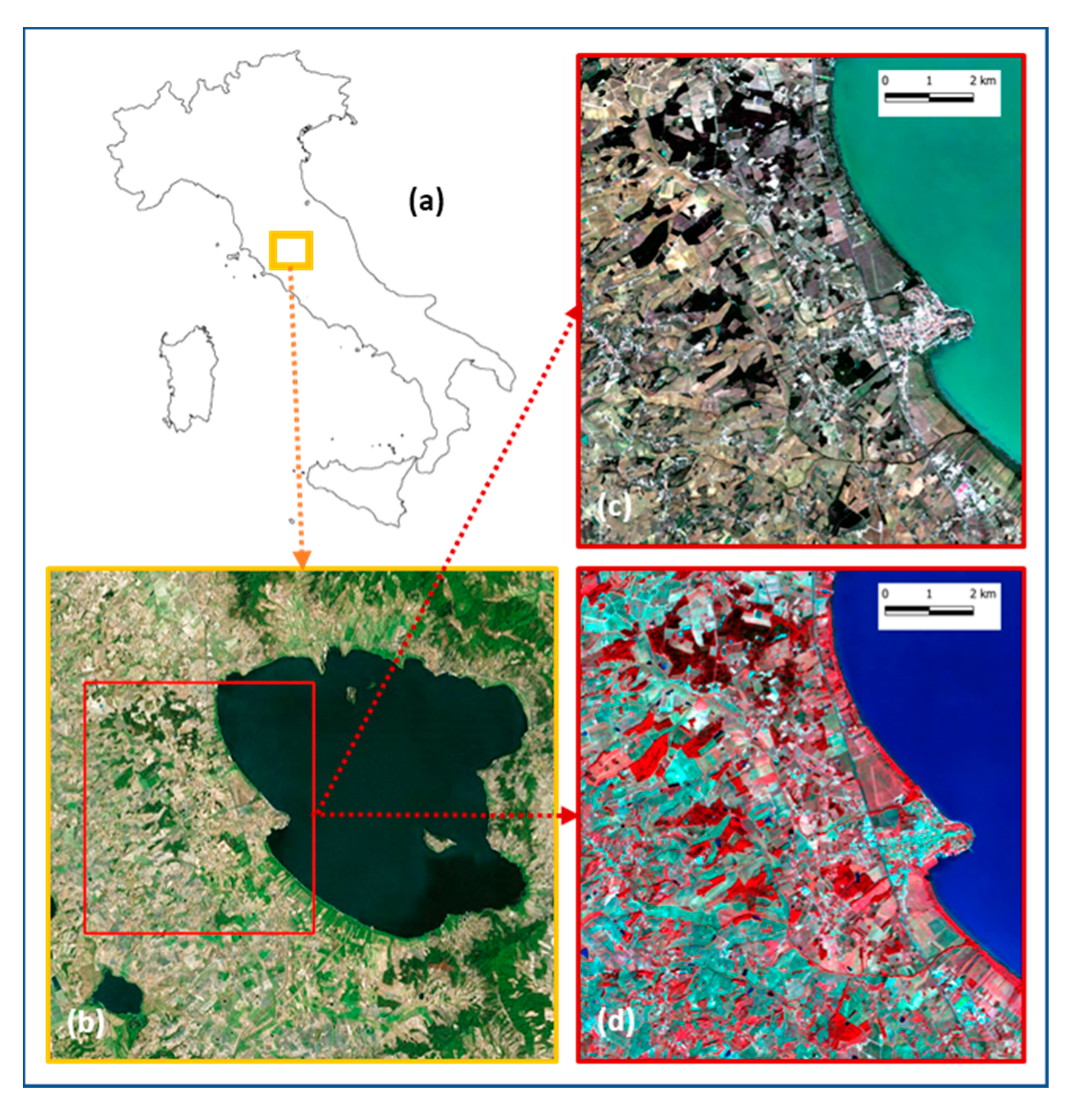
Figure 1. Study area location in Umbria, Italy (a) and overview of the Trasimeno Lake area (b). RGB image (c) and composite infrared image (d) based on 10 m resolution Sentinel 2 bands.
Remotesensing 12 03776 g001
Figure 2. The methodological workflow implemented in Google Earth Engine (GEE).
Remotesensing 12 03776 g002
Figure 3. RGB image, pixel-based (PB), and object-oriented (OO) Land Use–Land Cover (LULC) classifications of the study-area. (a) RGB image, (b) PB, (c) OO for Landsat 8; (d) RGB image, (e) PB, (f) OO for Sentinel 2; (g) RGB image, (h) PB, (i) OO for PlanetScope.
Remotesensing 12 03776 g003
Figure 4. RGB image, pixel-based (PB) classification, spatial cluster (SC) identified by Simple Non-Iterative Clustering (SNIC), and object-oriented (OO) classifications of a portion of the study-area. (a) RGB image, (b) PB, (c) SC, (d) OO for Landsat 8; (e) RGB image, (f) PB, (g) SC, (h) OO for Sentinel 2; (i) RGB image, (j) PB, (k) SC, (l) OO for PlanetScope.
Remotesensing 12 03776 g004
Figure 5. Percentages of the total area occupied by the LULC classes in the selected classifications (L8: Landsat 8, S2: Sentinel 2; PS: PlanetScope; PB: pixel-based; OO: object-oriented).
Remotesensing 12 03776 g005
Figure 6. Comparison of producer’s (a) and user’s (b) accuracies of the LULC classes from the selected classifications (L8: Landsat 8, S2: Sentinel 2; PS: PlanetScope; PB: pixel-based; OO: object-oriented). Woodlands and water LULC classes are omitted.
Remotesensing 12 03776 g006
Table 1. The number of validation points for each Land Use–Land Cover (LULC) class.
CLASSNumber of Validation Points
Built-up35
Annual crops154
Permanent crops40
Grasslands59
Woodlands65
Riparian Vegetation or Shrubs17
Water80
Total450
Table 2. List and short descriptions of the selected the Gray-Level Co-occurrence Matrix (GLCM) metrics.
BandsDescription
Angular Second Moment (ASM)Measures the uniformity or energy of the gray level distribution of the image
ContrastMeasures the contrast based on the local gray level variation
CorrelationMeasures the linear dependency of gray levels of neighboring pixels
EntropyMeasures the degree of the disorder among pixels in the image
VarianceMeasures the dispersion of the gray level distribution to emphasize the visual edges of land-cover patches
Inverse Difference Moment (IDM)Measures the smoothness (homogeneity) of the gray level distribution
Sum Average (SAVG)Measures the mean of the gray level sum distribution of the image
Table 3. Overall accuracies resulted from the pixel-based (PB) and object-oriented (OO) approaches, using data from three different satellite data (L8: Landsat 8; S2: Sentinel 2; PS: PlanetScope), applying the Random Forest (RF) or the Support Vector Machine (SVM) classifier, excluding or including textural information (GLCM) for the OO approach, using different seed spacing (5, 10, 15, 20 pixels for L8 and S2, and 35, 40, 45, 50 for PS-in italic), and. The best results from the PB and OO approaches, for the three datasets, are highlighted in bold.
SatClassifierPBOO Without GLCMOO With GLCM
5 (35)10 (40)15 (45)20 (50)5 (35)10 (40)15 (45)20 (50)
L8RF72.768.058.948.738.764.057.354.658.4
SVM79.178.471.361.173.170.467.661.364.4
S2RF8283.682.286.683.383.583.889.382.9
SVM80.280.984.285.382.483.886.286.984
PSRF74.27472.471.870.476.777.976.372.9
SVM74.872.473.170.970.874.973.973.671.7
Publisher’s Note: MDPI stays neutral with regard to jurisdictional claims in published maps and institutional affiliations.