Sea Echoes for Airborne HF/VHF Radar: Mathematical Model and Simulation

Abstract

Currently, shore-based HF radars are widely used for coastal observations, and airborne radars are utilized for monitoring the ocean with a relatively large coverage offshore. In order to take the advantage of airborne radars, the theoretical mechanism of airborne HF/VHF radar for ocean surface observation has been studied in this paper. First, we describe the ocean surface wave height with the linear and nonlinear parts in a reasonable mathematical form and adopt the small perturbation method (SPM) to compute the HF/VHF radio scattered field induced by the sea surface. Second, the normalized radar cross section (NRCS) of the ocean surface is derived by tackling the field scattered from the random sea as a stochastic process. Third, the NRCS is simulated using the SPM under different sea states, at various radar operating frequencies and incident angles, and then the influences of these factors on radar sea echoes are investigated. At last, a comparison of NRCS using the SPM and the generalized function method (GFM) is done and analyzed. The mathematical model links the sea echoes and the ocean wave height spectrum, and it also offers a theoretical basis for designing a potential airborne HF/VHF radar for ocean surface remote sensing.

1. Introduction

The sea echoes of HF or VHF ocean radars contain rich information about the sea surface since the length of the HF/VHF radio wave is very close to the wave length of gravity wave at the ocean surface [1]. On the one hand, shore-based HF radars are important components of coastal operational monitoring systems [2,3,4]. Many countries have utilized shore-based HF radars to obtain ocean current, wind and wave fields [5,6]. The maximum detection range of shore-based HF radars can reach 250 km, with the time resolution ranging from 10 min to 1 h and the spatial resolution varying from 300 m to 5 km. On the other hand, along with the development of electronic technology, airborne radars have been widely used for ocean remote sensing [7,8,9]. The size of radar is becoming smaller, and the cost of developing airborne radars is lower. In addition, an airborne VHF radar has been developed for forest remote sensing [10]. All these developments make it possible to design and develop an airborne HF/VHF radar to monitor the sea surface. The objective of this paper is to investigate the interaction mechanism of HF/VHF electromagnetic waves scattering from the ocean’s surface, and this should provide a theoretical basis for designing novel airborne HF/VHF radars for ocean remote sensing.

Many scholars have analyzed the interaction mechanism between HF/VHF electromagnetic waves and ocean waves for shore-based HF radar. Barrick [11] adopted the small perturbation method (SPM) to compute the scattered field from the time-varying sea surface and derived the normalized radar cross section (NRCS) of the sea surface for monostatic HF radar. Subsequently, Johnstone [12] and Anderson [13] respectively extended Barrick’s work to the configuration of shore-based bistatic HF radar. For the SPM, Hisaki [14] considered the effect of finite illumination area to derive the NRCS for shore-based monostatic HF radar. More recently, Hardman et al. [15] also presented the shore-based bistatic NRCS utilizing the SPM. Besides that, Srivastava and Walsh [16,17] proposed a generalized function method (GFM) to analyze the scattered field from the sea surface and derived the NRCS for the shore-based monostatic HF radar. Afterwards, the GFM was also extended to derive the NRCS for the shore-based bistatic HF radar [18,19,20]. It is noted that Silva et al. [21] modified the usual way of the GFM and derived a more general NRCS of the sea surface with arbitrary sea states.

For airborne HF/VHF radar, Bernhardt et al. [22,23] proposed the concept of HF Ground-Ionosphere- Ocean-Space (GIOS), and conducted experiments to observe the sea surface. Anderson [24] proposed the airborne passive HF radar which can be used to monitor the sea. Later, Chen et al. [25,26] theoretically analyzed the sea echoes of the shore-to-air bistatic HF radar. Meanwhile, Voronovich and Zavorotny [27] proved the possibility of extracting the wave height spectrum using airborne HF/VHF radars.

However, the theoretical study on the airborne HF/VHF radar is still in an initial stage. Voronovich and Zavorotny [27] analyzed the first-order interaction between HF/VHF radio waves and ocean waves, but they omitted the second-order information which is much more complicated than the first-order interaction and crucial for investigating the interaction mechanism between the HF/VHF radio waves and ocean surface waves. This paper analyzes the first- and second-order interactions which occur in the scattering of HF/VHF electromagnetic waves from the sea surface. First, a big square area of the sea surface is considered as the scattering patch. Taking into account the randomness of the sea surface, the ocean surface wave height is represented as the superposition of linear and nonlinear wave heights. Next, the SPM is employed to derive the scattered field from the sea surface. Then we obtain the NRCS of the sea surface for airborne HF/VHF radars. Finally, the theoretical NRCS of the sea surface is simulated with various parameters, such as sea states and radar operating frequencies.

This paper is organized as follows. Section 2 gives the description of the calculation of the scattered field. In Section 3, the NRCS of the sea surface is derived. Section 4 consists of the simulation of the NRCS and the analysis of the simulated sea echoes. Discussion and conclusions are presented in Section 5 and Section 6, respectively.

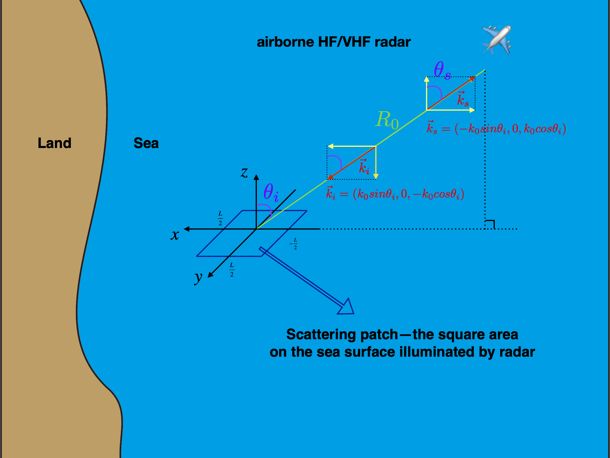
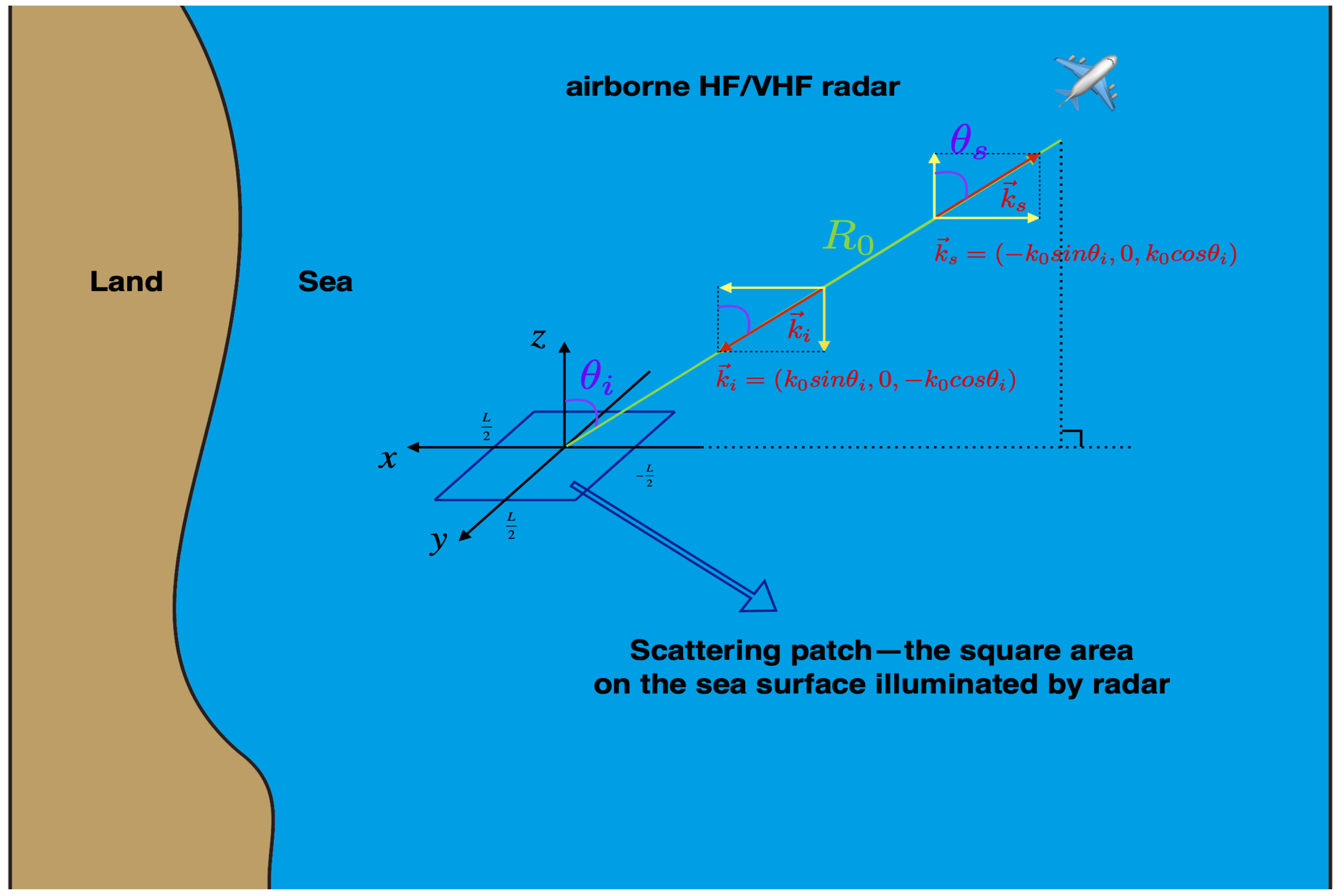
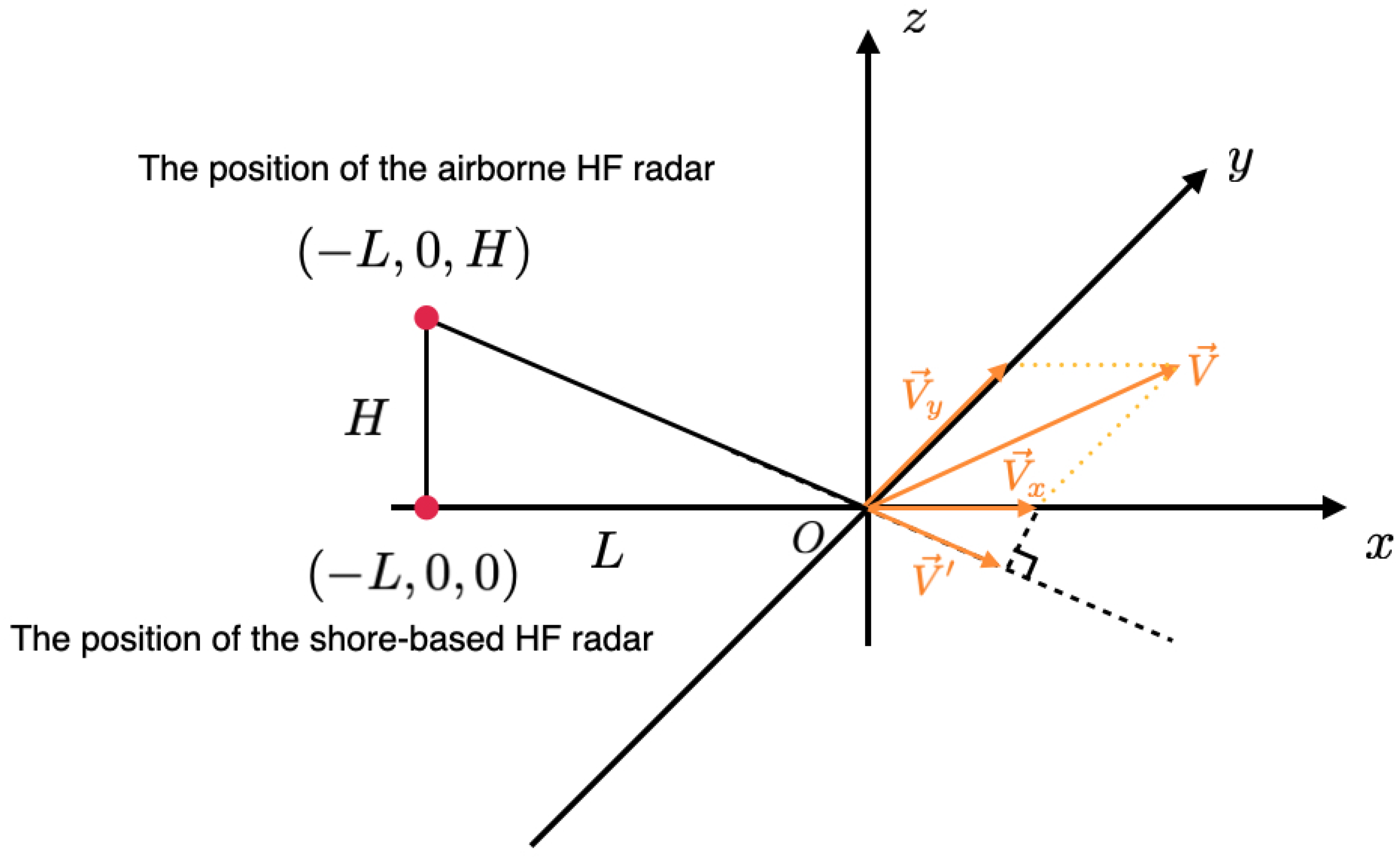
2. Description of the Scattering Problem

2.1. The Review of the Description of Wave Heights

As shown in Figure 1, the geometry of the scattering patch is established using a three-dimensional Cartesian coordinate system, and the center of the scattering patch is set as the origin. The scattering patch is assumed to be a square area with a very large side length of L. The x axis is assumed as the projection direction of radar beam at the sea surface and the y axis is at the sea surface and perpendicular to the x axis. The z axis is vertical to the sea surface.

Figure 1. The geometry of the scattering patch. The square scattering patch is represented by the parallelogram whose sides are navy blue straight lines. The radar is located in the far zone of the scattering patch ($R_0\gg L$). Backscattering is considered, i.e., ${\theta }_i={\theta }_s$. Here the x-z plane is perpendicular to the sea surface and contains the center of the scattering patch and the point of the radar position. $\overrightarrow{k_i}$ and $\overrightarrow{k_s}$ represent the wave vectors of the incident and scattered fields, respectively.

Then the sea surface wave height $z=f(x,y,t)$ can be expressed by Fourier series as:

$$\begin{array}{c}\hfill z=f(x,y,t)=f^{(1)}(x,y,t)+f^{(2)}(x,y,t),\end{array}$$

(1)

$$\begin{array}{c}\hfill f^{(1)}(x,y,t)=\sum _{m,n,l}^{}{p}_1(m,n,l)e^{iamx+iany-iwlt},\end{array}$$

(2)

$$\begin{array}{c}\hfill f^{(2)}(x,y,t)=\sum _{m,n,l}^{}{p}_2(m,n,l)e^{iamx+iany-iwlt},\end{array}$$

(3)

where m, n and l are integers between $-\infty$ and $+\infty$, $a=2\pi /L$ and $w=2\pi /T$; t denotes time; T is the temporal period of the Fourier expansion; $f^{(1)}(x,y,t)$ and $f^{(2)}(x,y,t)$ are Fourier series which denote linear and nonlinear wave heights [28], respectively; the superscripts 1 and 2 denote the first-order and second-order terms in the perturbational analysis, respectively; $p_1(m,n,l)$ and $p_2(m,n,l)$ are the Fourier coefficients of the linear and nonlinear wave heights, respectively.

When perturbational analysis is utilized to solve the hydrodynamic equations, it is found that $p_2(m,n,l)$ can be expressed using $p_1(m,n,l)$ [28]:

$$\begin{array}{c}\hfill p_2(m,n,l)=\sum _{m^{\prime },n^{\prime },l^{\prime }}^{}\mathsf{\Gamma }(\overrightarrow{k^{″}},{\omega }^{″},\overrightarrow{k^{\prime }},{\omega }^{\prime })p_1(m^{\prime },n^{\prime },l^{\prime })p_1(m-m^{\prime },n-n^{\prime },l-l^{\prime }),\end{array}$$

(4)

$$\begin{array}{c}\hfill (\overrightarrow{k^{″}},{\omega }^{″})=(a{m}^{\prime },a{n}^{\prime },w{l}^{\prime }),\end{array}$$

(5)

$$\begin{array}{c}\hfill (\overrightarrow{k^{\prime }},{\omega }^{\prime })=(am-a{m}^{\prime },an-a{n}^{\prime },wl-w{l}^{\prime }),\end{array}$$

(6)

where $m^{\prime }$, $n^{\prime }$ and $l^{\prime }$ are integers between $-\infty$ and $+\infty$; g is the gravitational acceleration; $\overrightarrow{k^{″}}$ and $\overrightarrow{k^{\prime }}$ represent two ocean wave vectors; ${\omega }^{″}$ and ${\omega }^{\prime }$ are the angular frequencies corresponding to $\overrightarrow{k^{″}}$ and $\overrightarrow{k^{\prime }}$, respectively. If $\overrightarrow{k^{″}}=-\overrightarrow{k^{\prime }}$ and ${\omega }^{″}=-{\omega }^{\prime }$, $\mathsf{\Gamma }(\overrightarrow{k^{″}},{\omega }^{″},\overrightarrow{k^{\prime }},{\omega }^{\prime })=0$; otherwise

$$\begin{array}{c}\hfill \mathsf{\Gamma }(\overrightarrow{k^{″}},{\omega }^{″},\overrightarrow{k^{\prime }},{\omega }^{\prime })=\frac{1}{2}\left[|\overrightarrow{k^{″}}|+|\overrightarrow{k^{\prime }}|+\frac{{\omega }_0^{″}{\omega }_0^{\prime }}{g}(1-\frac{\overrightarrow{k^{″}}·\overrightarrow{k^{\prime }}}{|\overrightarrow{k^{″}}||\overrightarrow{k^{\prime }}|})\frac{g|\overrightarrow{k^{″}}+\overrightarrow{k^{\prime }}|+{({\omega }_0^{″}+{\omega }_0^{\prime })}^2}{g|\overrightarrow{k^{″}}+\overrightarrow{k^{\prime }}|-{({\omega }_0^{″}+{\omega }_0^{\prime })}^2}\right],\end{array}$$

(7)

where $|\overrightarrow{k^{″}}|$ and $|\overrightarrow{k^{\prime }}|$ are the lengths of $\overrightarrow{k^{″}}$ and $\overrightarrow{k^{\prime }}$, respectively. The angular frequencies ${\omega }_0^{″}=\pm \sqrt{g|\overrightarrow{k^{″}}|}$ and ${\omega }_0^{\prime }=\pm \sqrt{g|\overrightarrow{k^{\prime }}|}$ are given by the dispersion relationship of the gravity waves in deep water.

2.2. Statistical Characteristics of the Scattering Patch

According to [29], the Fourier coefficient $p_1(m,n,l)$ of linear wave height can be considered as a Gaussian random variable so that (1)–(3) can represent a real random sea surface. The mean of the random variable $p_1(m,n,l)$ is zero:

$$\begin{array}{c}\hfill <p_1(m,n,l)>=0,\end{array}$$

(8)

where $<\cdots >$ denotes a statistical ensemble average. $p_2(m,n,l)$ is also a random variable, because $p_2(m,n,l)$ is determined by random variable $p_1(m,n,l)$.

The linear wave height $f^{(1)}(x,y,t)$ can be regarded as a stationary random process, so the power spectral density of the linear wave height is calculated as:

$$\begin{array}{c}\hfill W(p,q,\omega )=\frac{1}{{\pi }^3}{\int \int \int }_{-\infty }^{+\infty }<f^{(1)}(x_1,y_1,t_1)f^{(1)*}(x_2,y_2,t_2)>e^{-ip{\tau }_x-iq{\tau }_y-i\omega \tau }d{\tau }_{x}d{\tau }_{y}d\tau ,\end{array}$$

(9)

where ${\tau }_x=x_1-x_2$, ${\tau }_y=y_1-y_2$, $\tau =t_2-t_1$ and $f^{(1)*}(x_2,y_2,t_2)$ means the complex conjugation of $f^{(1)}(x_2,y_2,t_2)$. $W(p,q,\omega )$ is called the spatial-temporal spectrum of ocean waves. p and q denote the components of a ocean wave vector $\overrightarrow{k}$ along the x axis and y axis, respectively. $\omega$ is the angular frequency corresponding to $\overrightarrow{k}$. After calculation, the relationship between $W(p,q,\omega )$ and $p_1(m,n,l)$ is

$$\begin{array}{c}\hfill W(p,q,\omega )=\frac{L^{2}T}{{\pi }^3}<p_1(m,n,l),p_1^{*}(m,n,l)>,\end{array}$$

(10)

where $(\overrightarrow{k},\omega )=(p,q,\omega )=(am,an,wl)$. The spatial-temporal spectrum $W(p,q,\omega )$ also can be expressed as

$$\begin{array}{c}\hfill W(\overrightarrow{k},\omega )=4S(\overrightarrow{k})\delta (\omega -\sqrt{g|\overrightarrow{k}|})+4S(-\overrightarrow{k})\delta (\omega +\sqrt{g|\overrightarrow{k}|}),\end{array}$$

(11)

where $\delta (·)$ is the Dirac delta function, and $S(\overrightarrow{k})$ is the directional wavenumber spectrum.

2.3. The Incident and Scattered Fields Near the Sea Surface

Now we assume the incident field arriving at the scattering patch is vertically polarized with an incidence angle of ${\theta }_i$. The wave vector $\overrightarrow{k_i}=(k_{0}sin{\theta }_i,0,-k_{0}cos{\theta }_i)$ of the incident electromagtic wave is shown in Figure 1. Then the incident plane wave near the scattering patch, $\overrightarrow{E^i}$, can be expressed as:

$$\begin{array}{c}\hfill \overrightarrow{E^i}=E_0(cos{\theta }_i\widehat{x}+sin{\theta }_i\widehat{z})e^{i{k}_{0}sin{\theta }_{i}x-i{k}_{0}cos{\theta }_{i}z-i{\omega }_{c}t}=E_x^i\widehat{x}+E_y^i\widehat{y}+E_z^i\widehat{z},\end{array}$$

(12)

where $E_0$ is the magnitude of the electric field intensity of the incident field; ${\omega }_c$ and $k_0$ are the angular frequency and wavenumber corresponding to the radio frequency $f_c$ in the free space, respectively; $\widehat{x}$, $\widehat{y}$ and $\widehat{z}$ are unit vectors along each coordinate axis; $E_x^i$, $E_y^i$ and $E_z^i$ are the components of $\overrightarrow{E^i}$ along the x, y and z axes, respectively.

In (1)–(3), the whole sea surface has been treated as a periodic repetition of the scattering patch. In this way, the scattered field near the scattering patch can be derived using the SPM, which is a classical way to calculate the scattered field generated by periodic rough surface.

The slightly rough sea surface within the scattering patch can be divided into two parts: one is the planar part of the surface, and the other is the rough part of the surface. Consequently, the scattered field near the scattering patch contains two parts: the field induced by the planar surface, $\overrightarrow{E^{sp}}=E_x^{sp}\widehat{x}+E_y^{sp}\widehat{y}+E_z^{sp}\widehat{z}$, and the field caused by the rough surface, $\overrightarrow{E^{sr}}=E_x^{sr}\widehat{x}+E_y^{sr}\widehat{y}+E_z^{sr}\widehat{z}$. With the assumption that the sea water is an ideal conductor and the incident field is a plane wave at a frequency of $f_c$, the total electric field intensity, $\overrightarrow{E^t}=E_x^t\widehat{x}+E_y^t\widehat{y}+E_z^t\widehat{z}$, near the scattering patch, can be expressed as:

$$\begin{array}{c}\hfill \overrightarrow{E^t}=\overrightarrow{E^i}+\overrightarrow{E^{sp}}+\overrightarrow{E^{sr}}.\end{array}$$

(13)

The scattered field induced by the planar part is

$$\begin{array}{c}\hfill \overrightarrow{E^{sp}}=E_0(-cos{\theta }_i\widehat{x}+sin{\theta }_i\widehat{z})e^{i{k}_{0}sin{\theta }_{i}x+i{k}_{0}cos{\theta }_{i}z-i{\omega }_{c}t}.\end{array}$$

(14)

The components $E_x^{sr},E_y^{sr}$ and $E_z^{sr}$ of the scattered field induced by the rough part are expressed as Fourier series:

$$\begin{array}{c}\hfill \left\{\begin{array}{c}{E}_x^{sr}=\sum _{m,n,l}A(m,n,l)E(m,n,l),\hfill \\ E_y^{sr}=\sum _{m,n,l}B(m,n,l)E(m,n,l),\hfill \\ E_z^{sr}=\sum _{m,n,l}C(m,n,l)E(m,n,l),\hfill \end{array}\right.\end{array}$$

(15)

where $A(m,n,l),B(m,n,l)$ and $C(m,n,l)$ are unkown Fourier coefficients. $E(m,n,l)$ is assumed as:

$$\begin{array}{c}\hfill E(m,n,l)=E_0{e}^{iamx+iany+ib(m,n)z-i(wl+{\omega }_c)t},\end{array}$$

(16)

and $b(m,n)$ is defined as

$$\begin{array}{c}\hfill b(m,n)=\left\{\begin{array}{cc}\sqrt{k_0^2-a^2{m}^2-a^2{n}^2},\hfill & \mathrm{if}{m}^2+n^2<k_0^2/a^2\hfill \\ i\sqrt{a^2{m}^2+a^2{n}^2-k_0^2},\hfill & \mathrm{if}{m}^2+n^2>k_0^2/a^2\hfill \end{array}\right..\end{array}$$

(17)

The coefficients $A(m,n,l),B(m,n,l)$ and $C(m,n,l)$ can be derived by expanding boundary conditions in perturbation parameter or smallness [30]. Here $f^{(1)}(x,y,t)$ and $f^{(2)}(x,y,t)$ are selected as the first- and second-order smallness, respectively.

Two boundary conditions must be satisfied. First, the tangential component of the total electric field intensity is zero at the interface between the sea water and the air, because the sea water is perfectly conducting. Second, the divergence of the total electric field intensity is zero, because the zone above the sea surface is sourceless. Then substituting the components $E_x^t$, $E_y^t$ and $E_z^t$ of the total electric field into these two boundary conditions gives the first- and second-order solutions of $A(m,n,l)$, $B(m,n,l)$ and $C(m,n,l)$. The results are presented in (18)–(25) where $av=sin{\theta }_i$ with an integer v is assumed to facilitate the calculation. $A^{(1)}(m,n,l)$, $B^{(1)}(m,n,l)$ and $C^{(1)}(m,n,l)$ are the first-order solutions. $A^{(2)}(m,n,l)$, $B^{(2)}(m,n,l)$ and $C^{(2)}(m,n,l)$ are the second-order solutions. Substituting these Fourier coefficients into $E_x^{sr}$, $E_y^{sr}$ and $E_z^{sr}$, the total electric field near the sea surface can be obtained.

Referring to Barrick’s work [31], the first- and second-order terms of the scattered field are caused by the first- and second-order Bragg scattering, respectively.

$$\begin{array}{c}\hfill \left\{\begin{array}{c}A(m,n,l)=A^{(1)}(m,n,l)+A^{(2)}(m,n,l)\hfill \\ B(m,n,l)=B^{(1)}(m,n,l)+B^{(2)}(m,n,l)\hfill \\ C(m,n,l)=C^{(1)}(m,n,l)+C^{(2)}(m,n,l)\hfill \end{array}\right.\end{array}$$

(18)

$$\begin{array}{c}\hfill A^{(1)}(m,n,l)=2i(k_0-amsin{\theta }_i)p_1(m-v,n,l)\end{array}$$

(19)

$$\begin{array}{c}\hfill B^{(1)}(m,n,l)=-2iansin{\theta }_i{p}_1(m-v,n,l)\end{array}$$

(20)

$$\begin{array}{c}\hfill C^{(1)}(m,n,l)=\frac{1}{b(m,n)}2i[-k_{0}a(m-v)-b^2(m,n)sin{\theta }_i]p_1(m-v,n,l)\end{array}$$

(21)

$$\begin{array}{c}\hfill \begin{array}{c}\hfill A^{(2)}(m,n,l)=2i(k_0-amsin{\theta }_i)p_2(m-v,n,l)+\\ \hfill \sum _{m^{\prime },n^{\prime },l^{\prime }}2[(k_0-amsin{\theta }_i)b^2(m^{\prime },n^{\prime })+k_0(am-a{m}^{\prime })(av-a{m}^{\prime })]Q(m,n,l,m^{\prime },n^{\prime },l^{\prime })\end{array}\end{array}$$

(22)

$$\begin{array}{c}\hfill \begin{array}{c}\hfill B^{(2)}(m,n,l)=-2iansin{\theta }_i{p}_2(m-v,n,l)+\\ \hfill \sum _{m^{\prime },n^{\prime },l^{\prime }}2[k_0(an-a{n}^{\prime })(av-a{m}^{\prime })-ansin{\theta }_i{b}^2(m^{\prime },n^{\prime })]Q(m,n,l,m^{\prime },n^{\prime },l^{\prime })\end{array}\end{array}$$

(23)

$$\begin{array}{c}\hfill \begin{array}{c}\hfill C^{(2)}(m,n,l)=\frac{1}{b(m,n)}2i[-k_{0}a(m-v)-b^2(m,n)sin{\theta }_i]p_2(m-v,n,l)+\\ \hfill \frac{1}{b(m,n)}\sum _{m^{\prime },n^{\prime },l^{\prime }}2\{[a^2(m^2+n^2)sin{\theta }_i-am{k}_0]b^2(m^{\prime },n^{\prime })\}Q(m,n,l,m^{\prime },n^{\prime },l^{\prime })+\\ \hfill \frac{1}{b(m,n)}\sum _{m^{\prime },n^{\prime },l^{\prime }}2\{a^3{k}_0(m^{\prime }-v)(m^2+n^2-m{m}^{\prime }-n{n}^{\prime })\}Q(m,n,l,m^{\prime },n^{\prime },l^{\prime })\end{array}\end{array}$$

(24)

$$\begin{array}{c}\hfill Q(m,n,l,m^{\prime },n^{\prime },l^{\prime })=\frac{p_1(m^{\prime }-v,n^{\prime },l^{\prime })p_1(m-m^{\prime },n-n^{\prime },l-l^{\prime })}{b(m^{\prime },n^{\prime })}\end{array}$$

(25)

2.4. The Scattered Field Far from the Scattering Patch

For airborne HF radars, the antennas are located in the far zone of the scattering patch. As shown in Figure 1, the far zone means that the distance $R_0$ between the radar antenna and the center of the scattering patch is much longer than the side length L of the scattering patch.

Here the Stratton–Chu integral is employed to calculate the scattered field in the far zone of the scattering patch [12,32]. For monostatic configuration, substituting the scattered field from the rough part of the scattering patch into the Stratton–Chu integral gives (26), which represents the scattered field $\overrightarrow{H^f}(R_0,t)$ at the receive antenna.

$$\begin{array}{c}\hfill \begin{array}{c}\hfill \overrightarrow{H^f}(R_0,r)=\frac{i{e}^{i{k}_0{R}_0}}{4\pi R_0}{\int }_{-L/2}^{L/2}{\int }_{-L/2}^{L/2}\{\overrightarrow{k_s}\times (\widehat{n}\times \overrightarrow{H^{sr}})-k_0\sqrt{\frac{{ϵ}_0}{{\mu }_0}}(\widehat{n}\times \overrightarrow{E^{sr}})\\ \hfill +\sqrt{\frac{{ϵ}_0}{{\mu }_0}}\overrightarrow{k_s}·(\widehat{n}\times \overrightarrow{E^{sr}})\frac{\overrightarrow{k_s}}{k_0}\}{e}^{-i\overrightarrow{k_s}·\overrightarrow{r}}dxdy\end{array}\end{array}$$

(26)

In (26), $\overrightarrow{H^{sr}}$ denotes the magnetic field corresponding to $\overrightarrow{E^{sr}}$; $\overrightarrow{k_s}=(-k_{0}sin{\theta }_i,0,k_{0}cos{\theta }_i)$ is the wave vector of the scatterd field; the square area $\left\{(x,y,z)|-L/2\le x\le L/2,-L/2\le y\le L/2,z=0\right\}$ is the integration interval of the Stratton–Chu integral; $\widehat{n}=\widehat{z}$ is the unit normal vector of the integration plane; $\overrightarrow{r}=(x,y,z)$ is the vector pointing from the center of the scattering patch to any point in the integration area; ${ϵ}_0$ and ${\mu }_0$ are the electrical and magnetic permittivity of free space, respectively. For backscattering, the angle of reflection ${\theta }_s$ is identical to the angle of incidence ${\theta }_i$, i.e., ${\theta }_i={\theta }_s$. As mentioned in [14,15], when L is very big, i.e., $L\to +\infty$ is assumed, the integration interval of the Stratton–Chu integral can also be set as $\left\{(x,y,z)|-L/2\le x\le L/2,-L/2\le y\le L/2,z=f(x,y,t)\right\}$. The results of the NRCS are the same for these two cases of the integration interval.

As shown in Figure 1, the antenna locates at the point $(R_0,{\theta }_s={\theta }_i,{\varphi }_s=\pi )$ in the spherical coordinate system. The vertical polarization is considered herein. Thus the vertically polarized component of $\overrightarrow{H^f}(R_0,t)$ is the component of $\overrightarrow{H^f}(R_0,t)$ along the direction ${\varphi }_s=\pi$ in the spherical coordinate system:

$$\begin{array}{c}\hfill H_{{\varphi }_s}^f(R_0,t)=\overrightarrow{H^f}(R_0,t)·(-\widehat{y})=\sum _{m,n,l}\{\zeta (m,n,l)\frac{sin[(am+k_{0}sin{\theta }_i)L/2]sin(anL/2)}{(am+k_{0}sin{\theta }_i)an}\},\end{array}$$

(27)

$$\begin{array}{c}\hfill \zeta (m,n,l)=\frac{i{e}^{i{k}_0{R}_0}}{\pi R_0}{E}_0\sqrt{\frac{{ϵ}_0}{{\mu }_0}}\{\left[cos{\theta }_{i}b(m,n)+k_0\right]A(m,n,l)-amcos{\theta }_{i}C(m,n,l)\}{e}^{-i(wl+{\omega }_c)t}.\end{array}$$

(28)

3. The NRCS of the Scattering Patch for Backscattering

3.1. The Power Spectral Density of the Scattered Field

The normalized power spectral density of the vertically polarized component $H_{{\varphi }_s}^f(R_0,t)$ of the scattered field at the receive antenna can be calculated as follows:

• Obtain the time autocorrelation function $R(\tau )$. The time autocorrelation function of $H_{{\varphi }_s}^f(R_0,t)$ is defined as

  $$\begin{array}{c}\hfill R(\tau )=<H_{{\varphi }_s}^f(R_0,t_1)H_{{\varphi }_s}^{f*}(R_0,t_2)>,\end{array}$$

  (29)

  where $\tau =t_2-t_1$.
• Estimate the power spectral density. Take the Fourier transform of $R(\tau )$ and estimate the power density spectrum $R({\omega }^{″})$:

  $$\begin{array}{c}\hfill R({\omega }^{″})=\frac{1}{\pi }\int R(\tau )e^{-i{\omega }^{″}\tau }d\tau .\end{array}$$

  (30)
• Calculate the normalized power spectral density. The normalized power density spectrum $\sigma ({\omega }^{″})$ is derived by:

  $$\begin{array}{c}\hfill \sigma ({\omega }^{″})=R({\omega }^{″})·\frac{4\pi R_0^2}{L^2{H}_0^2},\end{array}$$

  (31)

  where $H_0=E_0\sqrt{{ϵ}_0/{\mu }_0}$ is the magnitude of the magnetic field intensity corresponding to the magnitude of the electric field intensity of the incident field. $\sigma ({\omega }^{″})$ is also called the NRCS of the sea surface. The normalization is applied to derive the range-independent NRCS at the sea surface area.

For an airborne HF/VHF radar, $\sigma ({\omega }^{″})$ is a function of the incidence angle ${\theta }_i$. For that ${\omega }_d={\omega }^{″}-{\omega }_c$ is the Doppler frequency, $\sigma ({\omega }^{″})$ is rewritten as $\sigma ({\omega }_d,{\theta }_i)$ which is given in (32)–(34). The definitions of the coefficients and vectors in (32)–(34) are given in (35)–(41). Here the velocity of airplane is assumed to be constant within the coherent integration time and has been left out.

$$\begin{array}{c}\hfill \sigma ({\omega }_d,{\theta }_i)={\sigma }^{(1)}({\omega }_d,{\theta }_i)+{\sigma }^{(2)}({\omega }_d,{\theta }_i),\end{array}$$

(32)

$$\begin{array}{c}\hfill {\sigma }^{(1)}({\omega }_d,{\theta }_i)=2^4\pi k_0^4{(1+{sin}^2{\theta }_i)}^2\sum _{m_1=\pm 1}S(-2m_{1}sin{\theta }_i\overrightarrow{k_0})\delta ({\omega }_d-m_1{\omega }_B),\end{array}$$

(33)

$$\begin{array}{c}\hfill \begin{array}{c}\hfill {\sigma }^{(2)}({\omega }_d,{\theta }_i)=2^4\pi k_0^4\sum _{m_1,m_2=\pm 1}\int \int {|(1+{sin}^2{\theta }_i){\mathsf{\Gamma }}_H+{\mathsf{\Gamma }}_{EM}|}^{2}S(m_1\overrightarrow{k_1})\\ \hfill S(m_2\overrightarrow{k_2})\delta ({\omega }_d-m_1\sqrt{g{k}_1}-m_2\sqrt{g{k}_2})dpdq,\end{array}\end{array}$$

(34)

$$\begin{array}{c}\hfill \overrightarrow{k_0}=(k_0,0),\end{array}$$

(35)

$$\begin{array}{c}\hfill {\omega }_B=\sqrt{2g{k}_{0}sin{\theta }_i},\end{array}$$

(36)

$$\begin{array}{c}\hfill \overrightarrow{k_1}=(p-k_{0}sin{\theta }_i,q),\end{array}$$

(37)

$$\begin{array}{c}\hfill \overrightarrow{k_2}=(-k_{0}sin{\theta }_i-p,-q),\end{array}$$

(38)

$$\begin{array}{c}\hfill \overrightarrow{k_1}+\overrightarrow{k_2}=-2sin{\theta }_i\overrightarrow{k_0},\end{array}$$

(39)

$$\begin{array}{c}\hfill {\mathsf{\Gamma }}_{EM}=\left[\frac{-(\overrightarrow{k_1}·\widehat{x})(\overrightarrow{k_2}·\widehat{x})+(1+{sin}^2{\theta }_i)[k_0^2{cos}^2{\theta }_i+\overrightarrow{k_1}·\overrightarrow{k_2}]}{\sqrt{k_0^2{cos}^2{\theta }_i+\overrightarrow{k_1}·\overrightarrow{k_2}}-k_0\Delta }\right],\end{array}$$

(40)

$$\begin{array}{c}\hfill \mathsf{\Gamma }(\overrightarrow{k},\omega ,\overrightarrow{k^{\prime }},{\omega }^{\prime })\underset{\overrightarrow{k^{″}}=\overrightarrow{k_1},\overrightarrow{k^{\prime }}=\overrightarrow{k_2}}{\overset{{\omega }_0^{″}+{\omega }_0^{\prime }={\omega }_d}{\to }}{\mathsf{\Gamma }}_H=\frac{1}{2}\left[|\overrightarrow{k_1}|+|\overrightarrow{k_2}|+m_1{m}_2\sqrt{|\overrightarrow{k_1}||\overrightarrow{k_2}|}(1-\frac{\overrightarrow{k_1}·\overrightarrow{k_2}}{|\overrightarrow{k_1}||\overrightarrow{k_2}|})\frac{2g{k}_{0}sin{\theta }_i+{\omega }_d^2}{2g{k}_{0}sin{\theta }_i-{\omega }_d^2}\right].\end{array}$$

(41)

Both the first- and second-order scattered fields are considered; therefore, $\sigma ({\omega }_d,{\theta }_i)$ consists of two parts: ${\sigma }^{(1)}({\omega }_d,{\theta }_i)$ and ${\sigma }^{(2)}({\omega }_d,{\theta }_i)$, which are called the first- and second-order NRCS of the sea surface, respectively. ${\sigma }^{(1)}({\omega }_d,{\theta }_i)$ comes from the first-order component of $\overrightarrow{E^{sr}}$, i.e., $A^{(1)}(m,n,l)$, $B^{(1)}(m,n,l)$ and $C^{(1)}(m,n,l)$, which are directly proportional to the $p_1(m-v,n,l)$. Hence, the first-order NRCS ${\sigma }^{(1)}({\omega }_d,{\theta }_i)$ is only caused by the first-order Bragg scattering. Similarly, ${\sigma }^{(2)}({\omega }_d,{\theta }_i)$ comes from the second-order components of $\overrightarrow{E^{sr}}$, i.e., $A^{(2)}(m,n,l)$, $B^{(2)}(m,n,l)$ and $C^{(2)}(m,n,l)$, which include $p_2(m-v,n,l)$ and $Q(m,n,l,m^{\prime },n^{\prime },l^{\prime })$. The $\mathsf{\Gamma }(\overrightarrow{k^{″}},{\omega }^{″},\overrightarrow{k^{\prime }},{\omega }^{\prime })$ in $p_2(m-v,n,l)$ (given in (7)) becomes the hydrodynamic coupling coefficient ${\mathsf{\Gamma }}_H$ which is given in (41). According to Barrick’s definitions [31], ${\mathsf{\Gamma }}_{EM}$ (given in (40)) is called the electromagnetic coupling coefficient which comes from the second-order scattered field composed of $Q(m,n,l,m^{\prime },n^{\prime },l^{\prime })$. It can be seen that both $p_2(m-v,n,l)$ and $Q(m,n,l,m^{\prime },n^{\prime },l^{\prime })$ are the products of $p_1(m^{\prime },n^{\prime },l^{\prime })$ and $p_1(m-m^{\prime },n-n^{\prime },l-l^{\prime })$. Thus the second-order NRCS ${\sigma }^{(2)}({\omega }_d,{\theta }_i)$ is a result of the second-order Bragg scattering.

There is a singularity in the denominator of ${\mathsf{\Gamma }}_{EM}$ when $k_0^2{cos}^2{\theta }_i+\overrightarrow{k_1}·\overrightarrow{k_2}$ becomes zero. The assumption that the sea water is perfectly conducting causes the singularity. A term, $-k_0\Delta$, is added in the denominator of ${\mathsf{\Gamma }}_{EM}$ to eliminate this singularity [12,33]. $\Delta$ is the normalized surface impedance which is a complex constant, i.e., $\Delta =0.011-i(0.012)$. The added term $-k_0\Delta$ means the small energy loss of HF electromagnetic waves traveling along the actual sea surface which is good at conducting rather than perfectly conducting.

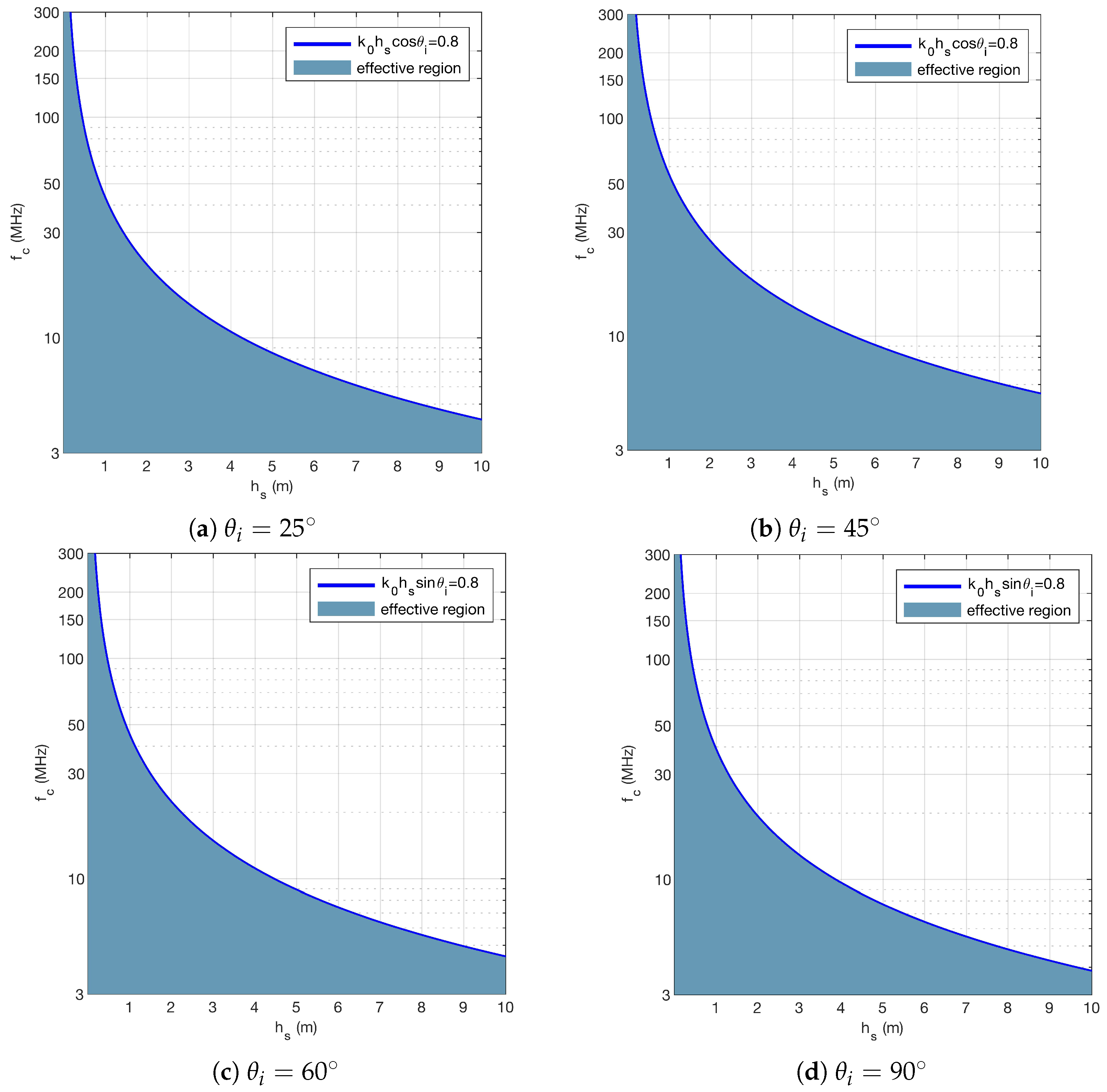
3.2. The Effectiveness of the NRCS

The NRCS of the sea surface has been derived using the SPM. Accordingly, the approximation made in the perturbational analysis must satisfy the condition:

$$\begin{array}{c}\hfill k_{0}hcos{\theta }_i\ll 0.5\mathrm{and}{k}_{0}hsin{\theta }_i\ll 0.5,\end{array}$$

(42)

where h is the root mean square (RMS) wave height of the sea surface, $k_0$ is the wavenumber of the incident plane wave at a frequency of $f_c$ and ${\theta }_i$ is the incident angle [28,34]. To ensure the correctness of the results from the perturbational analysis, a more rigorous condition is adopted in this work:

$$\begin{array}{c}\hfill k_{0}hcos{\theta }_i\le 0.2\mathrm{and}{k}_{0}hsin{\theta }_i\le 0.2.\end{array}$$

(43)

Considering that $h_s=4h$ ($h_s$ is significant wave height), the NRCS $\sigma ({\omega }_d,{\theta }_i)$ is effective only if the following inequality is satisfied:

$$\begin{array}{c}\hfill G(f_c)\le 0.8,\end{array}$$

(44)

where $G(f_c)$ is defined as:

$$\begin{array}{c}\hfill G(f_c)=\left\{\begin{array}{cc}{k}_0{h}_{s}cos{\theta }_i,\hfill & \mathrm{if}{20}^{\circ }\le {\theta }_i\le {45}^{\circ }\hfill \\ k_0{h}_{s}sin{\theta }_i,\hfill & \mathrm{if}{45}^{\circ }<{\theta }_i\le {90}^{\circ }\hfill \end{array}\right..\end{array}$$

(45)

The scattered field induced by the rough part of the sea surface is taken into consideration herein. As a result, the NRCS $\sigma ({\omega }_d,{\theta }_i)$ is effective only when the angle of incidence ${\theta }_i$ satisfies ${20}^{\circ }\le {\theta }_i\le {90}^{\circ }$ where the intensity of the scattered field from the plane part of the sea surface is much smaller than the intensity of the scattered field from the rough part of the sea surface [31]. Figure 2 shows the effective region of the NRCS $\sigma ({\omega }_d,{\theta }_i)$ in the $f_c-h_s$ plane with different ${\theta }_i$ values.

Figure 2. The effective region of the NRCS $\sigma ({\omega }_d,{\theta }_i)$. In (a) ${\theta }_i={25}^{\circ }$, (b) ${\theta }_i={45}^{\circ }$, (c) ${\theta }_i={60}^{\circ }$ and (d) ${\theta }_i={90}^{\circ }$, the area filled with dark blue is the effective region for each case.

4. The Simulation and Analysis of the Sea Echo

The interpretation of the NRCS of the sea surface is crucial to analyze the sea echoes. The NRCS of the sea surface, $\sigma ({\omega }_d,{\theta }_i)$, is interpreted as the theoretical prediction of the sea-echo Doppler spectrum. Consequently, the simulations of ${\sigma }^{(1)}({\omega }_d,{\theta }_i)$ and ${\sigma }^{(2)}({\omega }_d,{\theta }_i)$ are treated as the first- and second-order sea-echo Doppler spectra, respectively.

It can be found from the Formulas (32)–(34) that the directional wavenumber spectrum $S(\overrightarrow{k})$ is included in the theoretical sea-echo Doppler spectrum $\sigma ({\omega }_d,{\theta }_i)$. $S(\overrightarrow{k})$ is the product of a non-directional wave spectrum $S(k)$ and a directional distribution function $g(\alpha )$. It is assumed that only wind waves exist and they are fully developed. The Pierson–Moskowitz spectrum [35] and the cardioid distribution model [33] are assumed:

$$\begin{array}{c}\hfill S(\overrightarrow{k})=S(k)g(\alpha ),\end{array}$$

(46)

$$\begin{array}{c}\hfill S(k)=\frac{4.05\times {10}^{-3}}{k^4}{e}^{-0.74{(\frac{g}{k{U}^2})}^2},\end{array}$$

(47)

$$\begin{array}{c}\hfill g(\alpha )=\frac{{cos}^4(\frac{\alpha -{\alpha }^{\prime }}{2})}{{\int }_{-\pi }^{\pi }{cos}^4(\frac{\alpha }{2})d\alpha },\end{array}$$

(48)

where U is the wind speed at 19.5 m above the sea surface and ${\alpha }^{\prime }$ is the dominant wave direction which is the same with wind direction for wind-wave sea state. The relationship between U and $h_s$ is:

$$\begin{array}{c}\hfill h_s=4\sqrt{\int \int S(\overrightarrow{k})d\overrightarrow{k}}=0.2\frac{U^2}{g}.\end{array}$$

(49)

It can be seen that the theoretically predicted sea-echo Doppler spectrum $\sigma ({\omega }_d,{\theta }_i)$ is influenced by four factors: the dominant wave direction ${\alpha }^{\prime }$, the incident angle ${\theta }_i$, the radar frequency $f_c$ and the sea state $h_s$. Here we investigate the effects of the latter three factors on $\sigma ({\omega }_d,{\theta }_i)$. For simplification, a normalized Doppler frequency is defined as $\eta ={\omega }_d/{\omega }_B$ in the simulation. It is easy to prove that when ${\theta }_i={90}^{\circ }$, the theoretical sea-echo Doppler spectrum $\sigma ({\omega }_d,{\theta }_i)$ is reduced to the classical NRCS for shore-based HF radar.

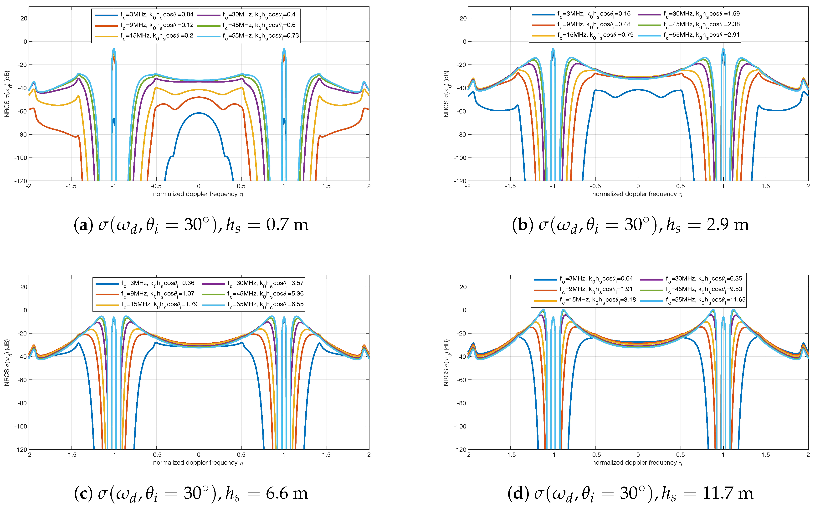
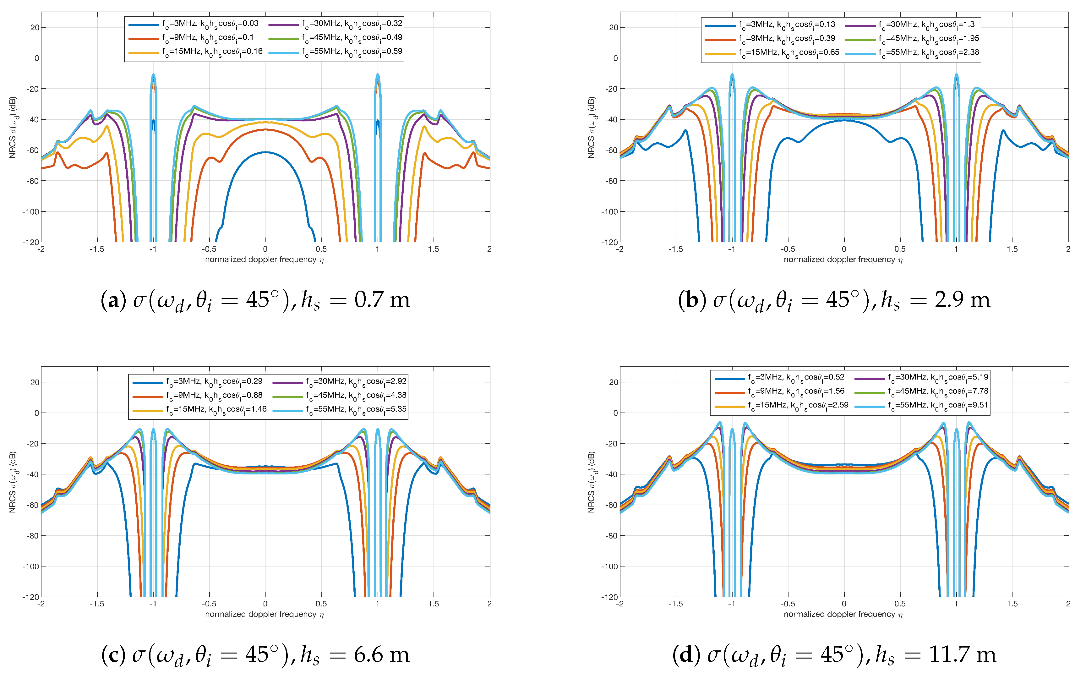
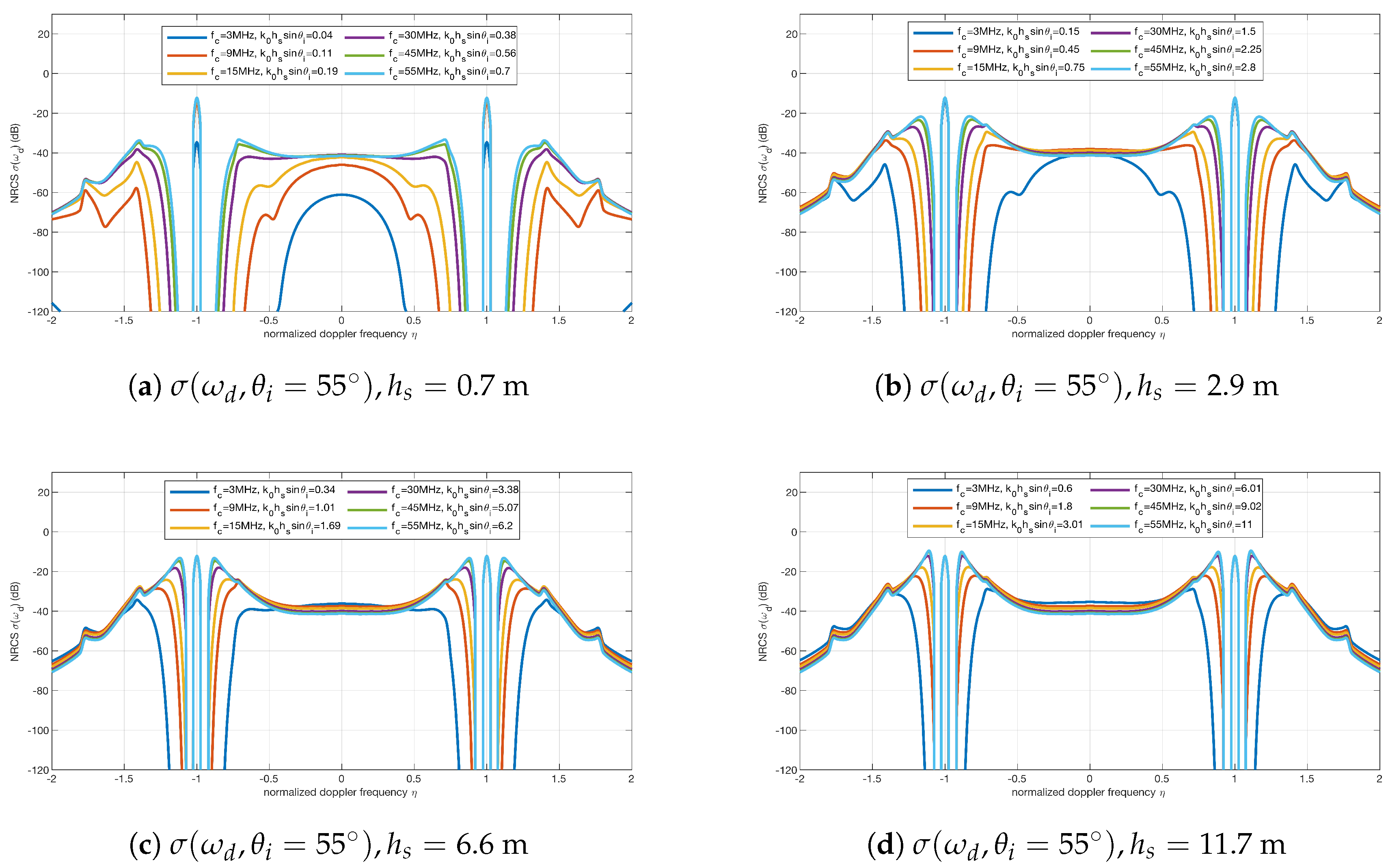
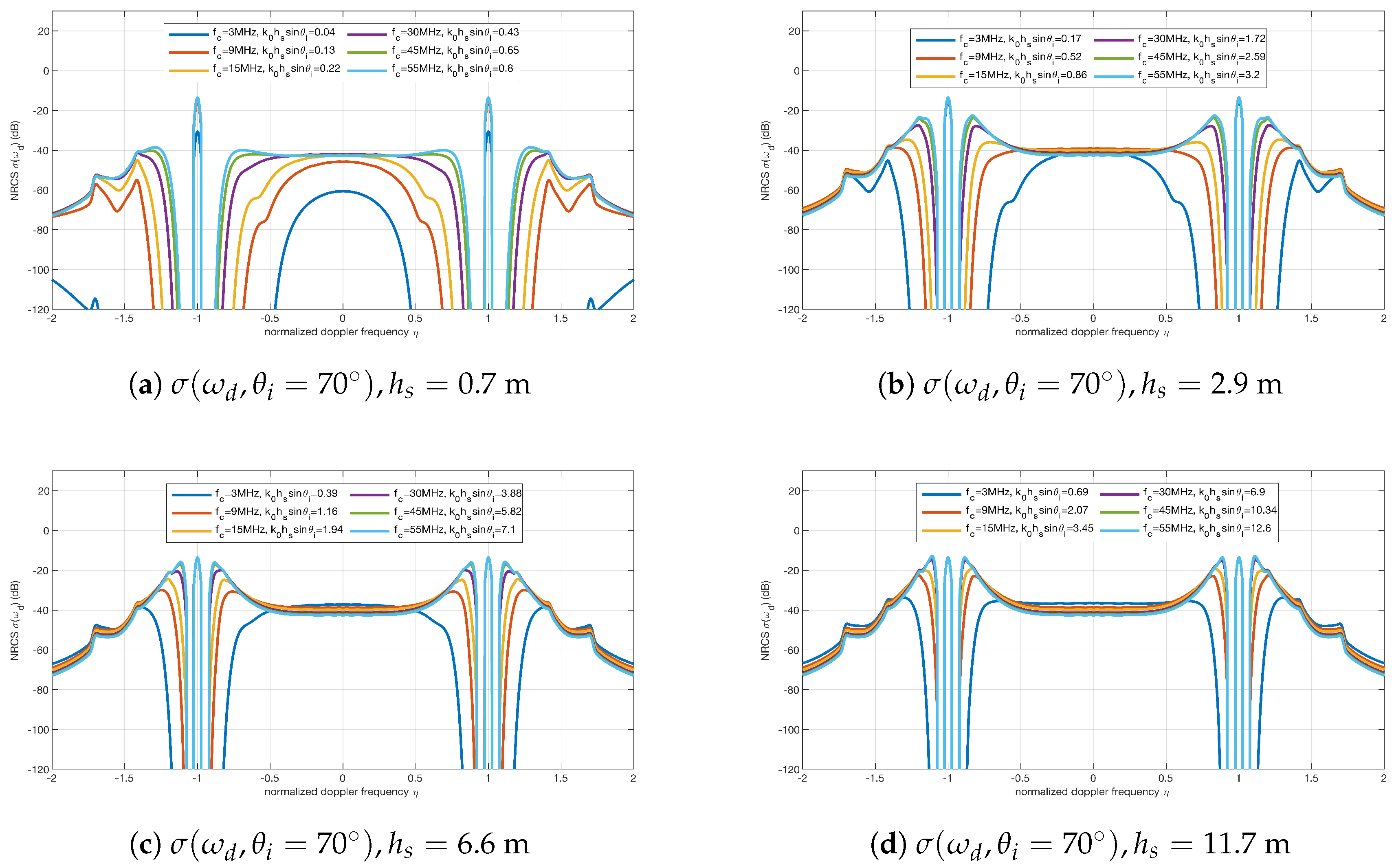
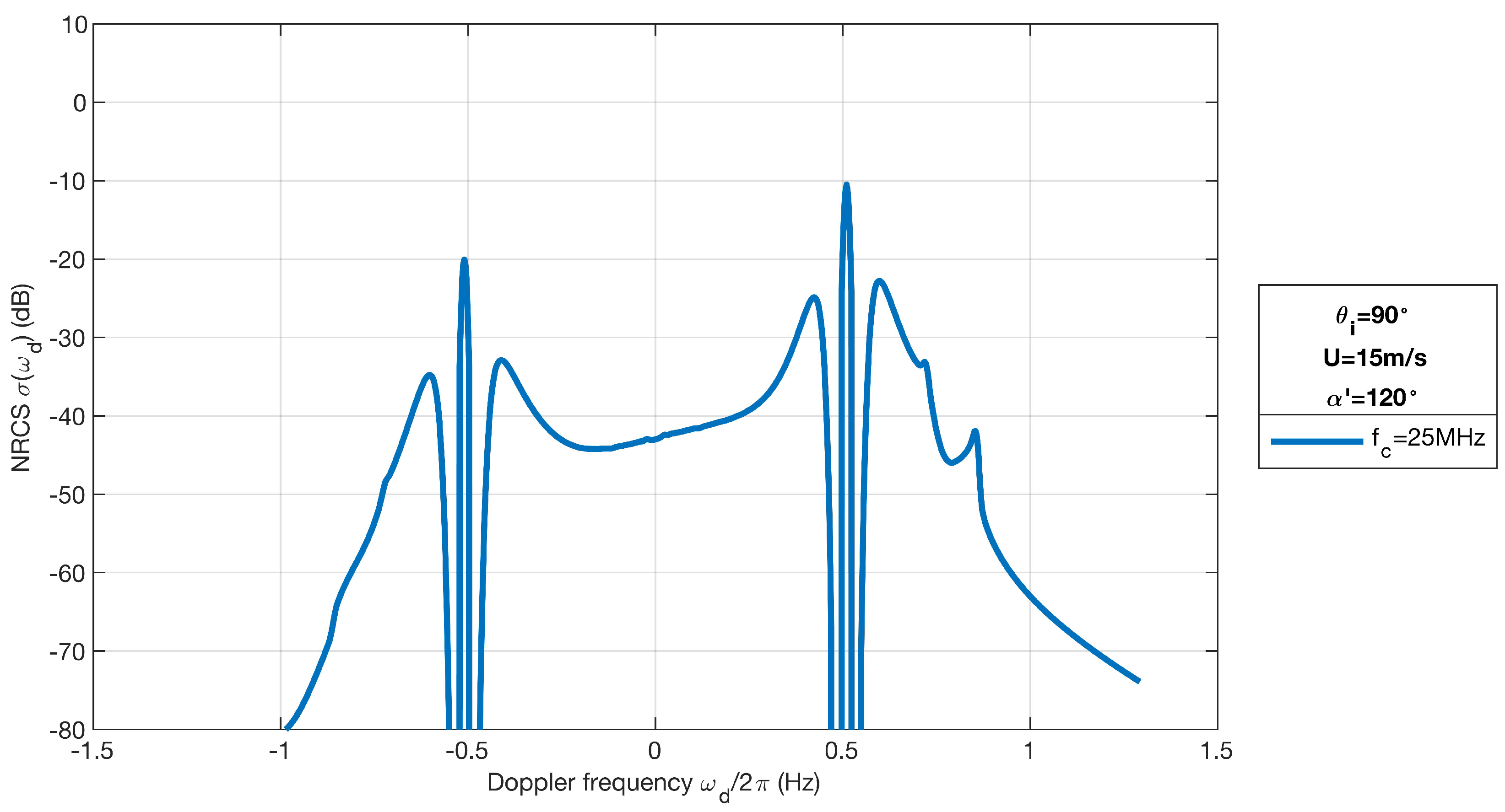
4.1. Sea Echoes at Different Radar Frequencies and Sea States

When ${\alpha }^{\prime }={90}^{\circ }$, different values of $f_c$, ${\theta }_i$ and $h_s$ are selected to simulate the Doppler spectrum. The simulated results for ${\theta }_i={30}^{\circ },{45}^{\circ },{55}^{\circ }$ and ${70}^{\circ }$ are given in Figure 3, Figure 4, Figure 5 and Figure 6, respectively. Each sub-figure in Figure 3, Figure 4, Figure 5 and Figure 6 corresponds to a combination of ${\theta }_i$ and $h_s$ and shows the Doppler spectrum at six radar frequencies, i.e., $f_c=$3, 9, 15, 30, 45 and 55 MHz. The first-order sea-echo Doppler spectrum ${\sigma }^{(1)}({\omega }_d,{\theta }_i)$ is represented by the two peaks at $\eta =\pm 1$, and the continuous curves around these two peaks are the second-order sea-echo Doppler spectra ${\sigma }^{(2)}({\omega }_d,{\theta }_i)$.

Figure 3. The Doppler spectra for ${\theta }_i={30}^{\circ }$ with different $f_c$ and $h_s$. (a) $\sigma ({\omega }_d,{\theta }_i={30}^{\circ }),h_s=0.7$ m; (b) $\sigma ({\omega }_d,{\theta }_i={30}^{\circ }),h_s=2.9$ m; (c) $\sigma ({\omega }_d,{\theta }_i={30}^{\circ }),h_s=6.6$ m; and (d) $\sigma ({\omega }_d,{\theta }_i={30}^{\circ }),h_s=11.7$ m. For each pair of ${\theta }_i$ and $h_s$, six radar frequencies were selected to simulate the spectra. The six values of $f_c$ were 3, 9, 15, 30, 45 and 55 MHz. The dominant wave direction ${\alpha }^{\prime }$ is ${90}^{\circ }$.

Figure 4. The Doppler spectra for ${\theta }_i={45}^{\circ }$ with different $f_c$ and $h_s$. (a) $\sigma ({\omega }_d,{\theta }_i={45}^{\circ }),h_s=0.7$ m; (b) $\sigma ({\omega }_d,{\theta }_i={45}^{\circ }),h_s=2.9$ m; (c) $\sigma ({\omega }_d,{\theta }_i={45}^{\circ }),h_s=6.6$ m; and (d) $\sigma ({\omega }_d,{\theta }_i={45}^{\circ }),h_s=11.7$ m. For each pair of ${\theta }_i$ and $h_s$, six radar frequencies were selected to simulate the spectra. The six values of $f_c$ were 3, 9, 15, 30, 45 and 55 MHz. The dominant wave direction ${\alpha }^{\prime }$ is ${90}^{\circ }$.

Figure 5. The Doppler spectra for ${\theta }_i={55}^{\circ }$ with different $f_c$ and $h_s$. (a) $\sigma ({\omega }_d,{\theta }_i={55}^{\circ }),h_s=0.7$ m; (b) $\sigma ({\omega }_d,{\theta }_i={55}^{\circ }),h_s=2.9$ m; (c) $\sigma ({\omega }_d,{\theta }_i={55}^{\circ }),h_s=6.6$ m; and (d) $\sigma ({\omega }_d,{\theta }_i={55}^{\circ }),h_s=11.7$ m. For each pair of ${\theta }_i$ and $h_s$, six radar frequencies were selected to simulate the spectra. The six values of $f_c$ were 3, 9, 15, 30, 45 and 55 MHz. The dominant wave direction ${\alpha }^{\prime }$ is ${90}^{\circ }$.

Figure 6. The Doppler spectra for ${\theta }_i={70}^{\circ }$ with different $f_c$ and $h_s$. (a) $\sigma ({\omega }_d,{\theta }_i={70}^{\circ }),h_s=0.7$ m; (b) $\sigma ({\omega }_d,{\theta }_i={70}^{\circ }),h_s=2.9$ m; (c) $\sigma ({\omega }_d,{\theta }_i={70}^{\circ }),h_s=6.6$ m; and (d) $\sigma ({\omega }_d,{\theta }_i={70}^{\circ }),h_s=11.7$ m. For each pair of ${\theta }_i$ and $h_s$, six radar frequencies were selected to simulate the spectra. The six values of $f_c$ were 3, 9, 15, 30, 45 and 55 MHz. The dominant wave direction ${\alpha }^{\prime }$ is ${90}^{\circ }$.

First, as shown in Figure 3, the symmetry characteristics of the simulated results (when ${\alpha }^{\prime }={90}^{\circ }$ and ${\theta }_i\ne {90}^{\circ }$) are the same as the simulated sea-echo Doppler spectra for shore-based HF radar (when ${\alpha }^{\prime }={90}^{\circ }$ and ${\theta }_i={90}^{\circ }$) [33].

Second, it is noted that the first-order sea-echo Doppler spectrum seems a constant for each ${\theta }_i$ when the radar works in a higher frequency band, e.g., $f_c\ge 15$ MHz. It can be found from Figure 3a, Figure 4a, Figure 5a and Figure 6a that the energy of the first-order peak is relatively smaller when radar frequency is low and sea state is calm, e.g., $f_c=3$ MHz and $h_s=0.7$ m. The reason for this is that the energy of ocean waves which cause the first-order Bragg scattering does not vary dramatically when $f_c$ is high and $h_s$ is large.

Finally, it can be seen from Figure 3a–d that the second-order spectrum increases in magnitude when $f_c$ increases. However, when the values of $f_c$ and $h_s$ do not meet the condition given in (44), the second-order spectrum is even higher than the first-order peaks. As mentioned in [33], in this case, the theoretical Doppler spectrum predicted by the SPM is not accurate.

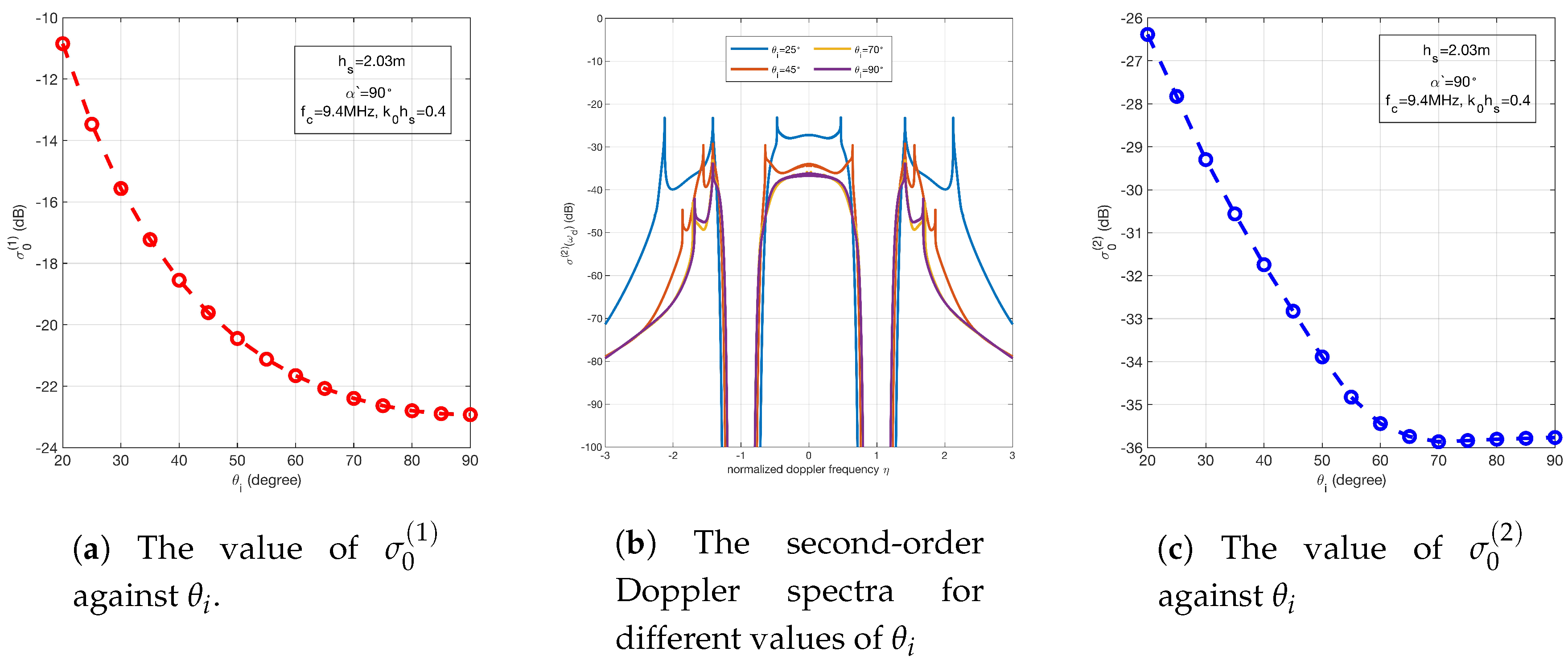
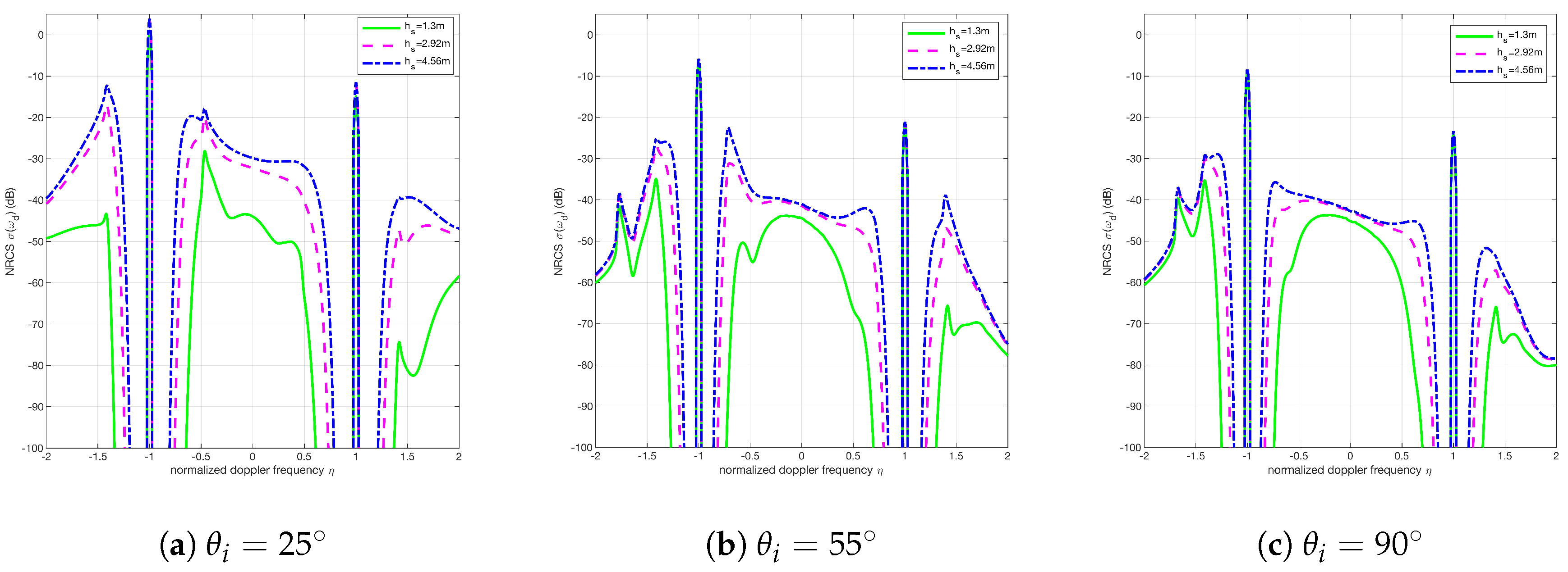
4.2. Sea Echoes for Different Incidence Angles

Comparing Figure 3a, Figure 4a, Figure 5a and Figure 6a, it can be found that the first-order spectrum ${\sigma }^{(1)}({\omega }_d,{\theta }_i)$, which is represented by the two highest peaks in the spectra, varies with ${\theta }_i$. To make it clear, the values of ${\sigma }_0^{(1)}=\frac{1}{2}{\int }_{-\infty }^{\infty }{\sigma }^{(1)}({\omega }_d,{\theta }_i)d{\omega }_d$ against incident angles are shown in Figure 7a, and it shows that the radar-received energy caused by the first-order Bragg scattering drops from $-11 \mathrm{dB}$ to $-23 \mathrm{dB}$ when ${\theta }_i$ increases from ${20}^{\circ }$ to ${90}^{\circ }$.

Figure 7. (a) The values of ${\sigma }_0^{(1)}$ for ${20}^{\circ }\le {\theta }_i\le {90}^{\circ }$. (b) The second-order Doppler spectra ${\sigma }^{(2)}({\omega }_d,{\theta }_i)$ for several incident angles ${\theta }_i$, i.e., ${\theta }_i={25}^{\circ },{45}^{\circ },{70}^{\circ }$ and ${90}^{\circ }$. (c) The values of ${\sigma }_0^{(1)}$ for ${20}^{\circ }\le {\theta }_i\le {90}^{\circ }$. $h_s=2.03 \mathrm{m}$, ${\alpha }^{\prime }={90}^{\circ }$ and $f_c=9.4 \mathrm{MHz}$ are assumed for (a), (b) and (c).

As shown in Figure 7b, this descending trend also exists in the second-order Doppler spectra for different ${\theta }_i$. For $|\eta |<1$, the values of second-order spectra decrease nearly 10 dB when ${\theta }_i$ varies from ${25}^{\circ }$ to ${90}^{\circ }$. In contrast, for $|\eta |>1$, the magnitude of the second-order spectrum decreases even more than 10 dB. Figure 7c demonstrates the value of ${\sigma }_0^{(2)}=\frac{1}{2}{\int }_{-\infty }^{\infty }{\sigma }^{(2)}({\omega }_d,{\theta }_i)d{\omega }_d$ against ${\theta }_i$, and it clearly shows the decrease in the radar-received energy caused by the second-order Bragg scattering.

However, this descending trend is not significant for the near-grazing case, i.e., for ${70}^{\circ }\le {\theta }_i\le {90}^{\circ }$. The value of ${\sigma }_0^{(1)}$ drops less than $1dB$ when ${\theta }_i$ changes from ${70}^{\circ }$ to ${90}^{\circ }$. The second-order Doppler spectrum for ${\theta }_i={70}^{\circ }$ is nearly identical to that for ${\theta }_i={90}^{\circ }$. Consequently, the values of ${\sigma }_0^{(2)}$ for ${\theta }_i={70}^{\circ }$ and ${90}^{\circ }$ are nearly equal. There are two reasons for this phenomenon. One reason is that the values of the functions $sin{\theta }_i$ and $cos{\theta }_i$ vary slightly with ${\theta }_i$ changing from ${70}^{\circ }$ to ${90}^{\circ }$, which causes a small variation in the length of the vector $-2sin{\theta }_i\overrightarrow{k_0}$. The other one is that the ocean waves which cause the second-order Bragg scattering contain nearly equal energy for ${70}^{\circ }\le {\theta }_i\le {90}^{\circ }$.

4.3. Sea Echoes for Different Sea States

In Section 4.1, it has been clearly seen that the first-order Doppler spectra do not vary as the sea state becomes higher. Here it is necessary to investigate the variation of the second-order spectrum when sea state is higher. As shown in Figure 8, the Doppler spectra under three different sea states ($h_s$ = 1.3 m, 2.92 m and 4.56 m) for different angles of incidence (${\theta }_i={25}^{\circ },{55}^{\circ }$ and ${90}^{\circ }$) were simulated while ${\alpha }^{\prime }={45}^{\circ }$ and $f_c=8\mathrm{MHz}$. It is obvious that the energy of the second-order Doppler spectrum becomes stronger along with the higher sea state.

Figure 8. The Doppler spectra for different values of $h_s$ and ${\theta }_i$. (a) ${\theta }_i={25}^{\circ }$. (b) ${\theta }_i={55}^{\circ }$. (c) ${\theta }_i={90}^{\circ }$. ${\alpha }^{\prime }={45}^{\circ }$ and $f_c=8 \mathrm{MHz}$. The Doppler spectra were simulated for three distinct values of $h_s$, i.e., $h_s=1.3 \mathrm{m},2.92 \mathrm{m}$ and $4.56 \mathrm{m}$. These three values of $h_s$ correspond to $U=8 \mathrm{m}/\mathrm{s}$, $12 \mathrm{m}/\mathrm{s}$ and $15 \mathrm{m}/\mathrm{s}$, respectively.

4.4. Comparison between SPM and GFM

For the case of shore-based monostatic HF radar, both the SPM [31] and GFM [16] have been utilized to derive the NRCS of the sea surface. For a comparison between these two methods, it is convenient to simulate the sea echoes derived by the two methods. Under the same condition as Figure 5 in [36], we simulated the model which was derived by using the SPM. The simulated result is shown in Figure 9.

Figure 9. The simulated Doppler spectrum for monostatic radar (${\theta }_i={90}^{\circ }$). In order to compare the simulated result with Figure 5 in [36], $U=15$ m/s, $f_c=25$ MHz and ${\alpha }^{\prime }={120}^{\circ }$ were assumed.

It is seen that the Doppler spectra simulated by the two methods are similar in shape. Each result shows that the positive first-order peak is nearly 10 dB larger than the negative one. However the amplitudes of these two spectra are not equal. As mentioned in [36], these two methods are different although they have the same form. The significant difference is that the NRCS based on the GFM is affected by the range resolution of the radar while the NRCS derived using the SPM is not based on this parameter.

The above comparison shows a typical example of the NRCSs simulated using the GFM and the SPM. However, a recent work [21] seems to indicate that the derivation of the NRCS using the GFM has a wider application range in terms of approximation restrictions. The derivation of the NRCS using the SPM is on the basis of three assumptions: first, the sea water is a good conductor; second, the slope of ocean surface wave height is much smaller than 1; third, the product of the significant wave height and the radio wavenumber is small. The results in Figure 3, Figure 4, Figure 5, Figure 6, Figure 7 and Figure 8 were obtained based on those conditions. Additionally, HF radar NRCS simulated using the SPM has been validated using real data for more than 50 years. In contrast, it is possible to remove the significant wave height restriction using the GFM as shown in [21]. In that work, the NRCS with arbitrary roughness scales has been obtained, but it has not been compared with real Doppler spectrum.

5. Discussion

Four factors, radar frequency $f_c$, the angle of incidence ${\theta }_i$, the significant wave height $h_s$ and the dominant wave direction ${\alpha }^{\prime }$, which influence the shape and the magnitude of the sea-echo Doppler spectrum, have been investigated.

First, it was found that the first- and second-order spectra increase when radar frequency becomes higher. However, the Doppler spectrum becomes saturated when radar frequency is too high to meet the effective condition of the SPM. From the radar equation, we know that $SN{R}_o\propto P_t{\sigma }_0/L_p$, where $SN{R}_o$ is the signal to noise ratio at the output of the radar receiver, $P_t$ is the transmitted power of radar, ${\sigma }_0=\frac{1}{2}{\int }_{-\infty }^{+\infty }\sigma ({\omega }_d,\theta )d{\omega }_d$ and $L_p$ represents the propagation loss of radio waves. If radar frequency increases, both the $L_p$ and ${\sigma }_0$ vary. Thus, it is much better to combine the ${\sigma }_0$ (derived in this paper) with a suitable $L_p$ (which is not the focus of our work) to select radar frequency for designing an airborne HF/VHF radar for ocean remote sensing.

Second, the variation that occurs in the sea-echo Doppler spectrum when ${\theta }_i$ changes attracts our attention. It can be known from Figure 7a,c that ${\sigma }_0$ increases nearly 10 dB with ${\theta }_i$ changing from ${90}^{\circ }$ to ${20}^{\circ }$ (${\sigma }_0={\sigma }_0^{(1)}+{\sigma }_0^{(2)}$). The ${\sigma }_0$ becomes large when the incident angle becomes small, and $L_p$ is smaller when radio waves propagate in the air than when they propagate along the air–sea surface. Consequently, considering the same $SN{R}_o$ for the airborne HF/VHF radar and the shore-based HF radar, $P_t$ could be much smaller for airborne HF/VHF radars. It is convenient to design a relatively compact and low-power airborne HF/VHF radar.

Third, the energy of the sea echo increases when the sea state becomes higher, which is similar to the case of shore-based HF radar.

Finally, since the NRCS connects the sea echoes and the waveheight spectrum, it is possible to retrieve wave parameters from radar sea echoes by inversing the NRCS. In addition, sea surface current may also be extracted from the first-order echoes by determining the Doppler shift induced by current. The difference between ${\theta }_i\ne {90}^{\circ }$ and ${\theta }_i={90}^{\circ }$ for current inversion is shown in Figure 10. If airborne and shore-based HF radars are located at the positions as the red points in the picture, the current velocity measured by the shore-based HF radar is ${\overrightarrow{V}}_x$, whereas the current measured by the airborne radar is ${\overrightarrow{V}}^{\prime }$ which is a component of ${\overrightarrow{V}}_x$.

Figure 10. The difference between ${\theta }_i\ne {90}^{\circ }$ and ${\theta }_i={90}^{\circ }$ for current inversion. A current with velocity vector $\overrightarrow{V}$ exists at the origin O. The airborne and shore-based HF radars are located at $(-L,0,H)$ and $(-L,0,0)$, respectively.

6. Conclusions

In this paper, the sea surface wave height has been expressed as the superposition of two Fourier series which represent linear and nonlinear wave heights. Then the SPM was adopted to get the scattered field from the sea surface. The scattered field has been calculated by taking into account both the first- and second-order Bragg scatterings between the sea surface waves and the electromagnetic waves. At last, theoretical models of the first- and second-order sea-echo Doppler spectra for the airborne HF/VHF radars have been derived. Besides that, the effectiveness region of the theoretical sea-echo Doppler spectrum $\sigma ({\omega }_d,{\theta }_i)$ was given.

There are continuous second-order spectra ${\sigma }^{(2)}({\omega }_d,{\theta }_i={90}^{\circ })$ around the first-order Bragg peaks ${\sigma }^{(1)}({\omega }_d,{\theta }_i={90}^{\circ })$ in the sea-echo Doppler spectra of the shore-based HF radar, and the continuous spectra have been used for wave parameter inversion in practice. Thus, the second-order terms in the SPM are not neglected in order to get the theoretical second-order sea-echo Doppler spectrum for the airborne HF/VHF radar. Both the first- and second-order spectra were simulated under different environment conditions to give a brief demonstration of the sea echo is received by radar. In addition, the results of the simulated sea echoes may provide a basic guide for designing an airborne HF/VHF radar to monitor the sea state in the future.

References

- Crombie, D.D. Doppler spectrum of sea echo at 13.56 Mc./s. Nature 1955, 175, 681–682. [Google Scholar] [CrossRef]
- Prandle, D.; Ryder, D. Measurement of surface currents in Liverpool Bay by high-frequency radar. Nature 1985, 315, 128–131. [Google Scholar] [CrossRef]
- Georges, T.; Harlan, J.; Lematta, R. Large-scale mapping of ocean surface currents with dual over-the-horizon radars. Nature 1996, 379, 434–436. [Google Scholar] [CrossRef]
- Zhao, C.; Chen, Z.; He, C.; Xie, F.; Chen, X. A Hybrid Beam-Forming and Direction-Finding Method for Wind Direction Sensing Based on HF Radar. IEEE Trans. Geosci. Remote Sens. 2018, 56, 6622–6629. [Google Scholar] [CrossRef]
- Capodici, F.; Cosoli, S.; Ciraolo, G.; Nasello, C.; Maltese, A.; Poulain, P.M.; Drago, A.; Azzopardi, J.; Gauci, A. Validation of HF radar sea surface currents in the Malta-Sicily Channel. Remote Sens. Environ. 2019, 225, 65–76. [Google Scholar] [CrossRef]
- Zhao, C.; Chen, Z.; Li, J.; Zhang, L.; Huang, W.; Gill, E.W. Wind Direction Estimation Using Small-Aperture HF Radar Based on a Circular Array. IEEE Trans. Geosci. Remote Sens. 2020, 58, 2745–2754. [Google Scholar] [CrossRef]
- Jackson, G.; Fornaro, G.; Berardino, P.; Esposito, C.; Lanari, R.; Pauciullo, A.; Reale, D.; Zamparelli, V.; Perna, S. Experiments of sea surface currents estimation with space and airborne SAR systems. In Proceedings of the 2015 IEEE International Geoscience and Remote Sensing Symposium (IGARSS), Milan, Italy, 26–31 July 2015; pp. 373–376. [Google Scholar]
- Forget, P.; Broche, P. Slicks, waves, and fronts observed in a sea coastal area by an X-band airborne synthetic aperture radar. Remote Sen. Environ. 1996, 57, 1–12. [Google Scholar] [CrossRef]
- Martin, A.C.; Gommenginger, C. Towards wide-swath high-resolution mapping of total ocean surface current vectors from space: Airborne proof-of-concept and validation. Remote Sens. Environ. 2017, 197, 58–71. [Google Scholar] [CrossRef]
- Israelsson, H.; Ulander, L.M.H.; Askne, J.L.H.; Fransson, J.E.S.; Frolind, P.; Gustavsson, A.; Hellsten, H. Retrieval of forest stem volume using VHF SAR. IEEE Trans. Geosci. Remote Sens. 1997, 35, 36–40. [Google Scholar] [CrossRef]
- Barrick, D. First-order theory and analysis of MF/HF/VHF scatter from the sea. IEEE Trans. Antennas Propag. 1972, 20, 2–10. [Google Scholar] [CrossRef]
- Johnstone, D.L. Second-Order Electromagnetic and Hydrodynamic Effects in High-Frequency Radio-Wave Scattering from the Sea. Ph.D. Thesis, Stanford Univeristy, Stanford, CA, USA, 1975. [Google Scholar]
- Anderson, S.J. Directional wave spectrum measurement with multistatic HF surface wave radar. In Proceedings of the IGARSS 2000. IEEE 2000 International Geoscience and Remote Sensing Symposium. Taking the Pulse of the Planet: The Role of Remote Sensing in Managing the Environment. Proceedings (Cat. No.00CH37120), Honolulu, HI, USA, 24–28 July 2000; Volume 7, pp. 2946–2948. [Google Scholar]
- Hisaki, Y.; Tokuda, M. VHF and HF sea echo Doppler spectrum for a finite illuminated area. Radio Sci. 2001, 36, 425–440. [Google Scholar] [CrossRef]
- Hardman, R.L.; Wyatt, L.R.; Engleback, C.C. Measuring the Directional Ocean Spectrum from Simulated Bistatic HF Radar Data. Remote Sens. 2020, 12, 313. [Google Scholar] [CrossRef]
- Srivastava, S.K. Scattering of High-Frequency Electromagnetic Waves from an Ocean Surface: An Alternative Approach Incorporating a Dipole Source. Ph.D. Thesis, Memorial University of Newfoundland, Saint John, NL, Canada, 1984. [Google Scholar]
- Srivastava, S.; Walsh, J. An alternate of HF Scattering from an ocean surface. In Proceedings of the 1983 Antennas and Propagation Society International Symposium, Houston, TX, USA, 23–26 May 1983; Volume 21, pp. 680–683. [Google Scholar]
- Gill, E.W.; Walsh, J. High-frequency bistatic cross sections of the ocean surface. Radio Sci. 2001, 36, 1459–1475. [Google Scholar] [CrossRef]
- Huang, W. The Second-Order High Frequency Bistatic Radar Cross Section of the Ocean Surface for Patch Scatter. Master’s Thesis, Memorial University of Newfoundland, Saint John, NL, Canda, 2004. [Google Scholar]
- Ma, Y.; Gill, E.W.; Huang, W. Bistatic High-Frequency Radar Ocean Surface Cross Section Incorporating a Dual-Frequency Platform Motion Model. IEEE J. Ocean. Eng. 2018, 43, 205–210. [Google Scholar] [CrossRef]
- Silva, M.T.; Huang, W.; Gill, E.W. High-Frequency Radar Cross-Section of the Ocean Surface with Arbitrary Roughness Scales: A Generalized Functions Approach. IEEE Trans. Antennas Propag. 2020. [Google Scholar] [CrossRef]
- Bernhardt, P.A.; Briczinski, S.J.; Siefring, C.L.; Barrick, D.E.; Bryant, J.; Howarth, A.; James, G.; Enno, G.; Yau, A. Large area sea mapping with Ground-Ionosphere-Ocean-Space (GIOS). In Proceedings of the OCEANS 2016 MTS/IEEE Monterey, Monterey, CA, USA, 19–23 September 2016; pp. 1–10. [Google Scholar]
- Bernhardt, P.A.; Siefring, C.L.; Briczinski, S.C.; Vierinen, J.; Miller, E.; Howarth, A.; James, H.G.; Blincoe, E. Bistatic observations of the ocean surface with HF radar, satellite and airborne receivers. In Proceedings of the OCEANS 2017, Anchorage, AK, USA, 18–21 September 2017; pp. 1–5. [Google Scholar]
- Anderson, S.J. Space-borne Passive HF Radar for Surveillance and Remote Sensing. In Proceedings of the Progress In Electromagnetics Research Symposium, St Petersburg, Russia, 22–25 May 2017; p. 1649. [Google Scholar]
- Zhao, C.; Chen, Z. Model of shore-to-air bistatic HF radar for ocean observation. In Proceedings of the OCEANS 2018 MTS/IEEE Charleston, Charleston, SC, USA, 22–25 October 2018; pp. 1–4. [Google Scholar]
- Chen, Z.; Li, J.; Zhao, C.; Ding, F.; Chen, X. The Scattering Coefficient for Shore-to-Air Bistatic High Frequency (HF) Radar Configurations as Applied to Ocean Observations. Remote Sens. 2019, 11, 2978. [Google Scholar] [CrossRef]
- Voronovich, A.G.; Zavorotny, V.U. Measurement of Ocean Wave Directional Spectra Using Airborne HF/VHF Synthetic Aperture Radar: A Theoretical Evaluation. IEEE Trans. Geosci. Remote Sens. 2017, 55, 3169–3176. [Google Scholar] [CrossRef]
- Weber, B.L.; Barrick, D.E. On the Nonlinear Theory for Gravity Waves on the Ocean’s Surface. Part I: Derivations. J. Phys. Oceanogr. 1977, 7, 3–10. [Google Scholar] [CrossRef]
- Barrick, D.E.; Weber, B.L. On the Nonlinear Theory for Gravity Waves on the Ocean’s Surface. Part II: Interpretation and Applications. J. Phys. Oceanogr. 1977, 7, 11–21. [Google Scholar] [CrossRef]
- Rice, S.O. Reflection of electromagnetic waves from slightly rough surfaces. Commun. Pure Appl. Math. 1951, 4, 351–378. [Google Scholar] [CrossRef]
- Barrick, D.E. Remote Sensing of Sea State by Radar. In Remote Sensing of the Troposphere; Derr, V.E., Ed.; U.S. Govt. Printing Office: Washington, DC, USA, 1972; pp. 1–46. [Google Scholar]
- Barrick, D.E. The interaction of HF/VHF radio waves with the sea surface and its implications. In Electromagnetic of the Sea, AGARD Conference Proceedings; AGARD: Neuilly sur Seine, France, 1970. [Google Scholar]
- Lipa, B.J.; Barrick, D.E. Extraction of sea state from HF radar sea echo: Mathematical theory and modeling. Radio Sci. 1986, 21, 81–100. [Google Scholar] [CrossRef]
- Barrick, D.E.; Peake, W.H. A review of scattering from surfaces with different roughness scales. Radio Sci. 1968, 3, 865–868. [Google Scholar] [CrossRef]
- Katopodes, N.D. Air-Water Interface. In Free-Surface Flow:Shallow Water Dynamics; Elsevier: Amsterdam, The Netherlands, 2019; Chapter 2; pp. 44–121. [Google Scholar]
- Gill, E.; Huang, W.; Walsh, J. On the Development of a Second-Order Bistatic Radar Cross Section of the Ocean Surface: A High-Frequency Result for a Finite Scattering Patch. IEEE J. Ocean. Eng. 2006, 31, 740–750. [Google Scholar] [CrossRef]
Publisher’s Note: MDPI stays neutral with regard to jurisdictional claims in published maps and institutional affiliations. |
© 2020 by the authors. Licensee MDPI, Basel, Switzerland. This article is an open access article distributed under the terms and conditions of the Creative Commons Attribution (CC BY) license (http://creativecommons.org/licenses/by/4.0/).