Article

Remote Sensing of Ice Conditions in the Southeastern Baltic Sea and in the Curonian Lagoon and Validation of SAR-Based Ice Thickness Products

by
Igor E. Kozlov
1,2,*,
Elena V. Krek
3,
Andrey G. Kostianoy
3,4,5 and
Inga Dailidienė
2,6
1
Satellite Oceanography Laboratory, Russian State Hydrometeorological University, Malookhtinsky pr. 98, St. Petersburg 195196, Russia
2
Marine Research Institute, Klaipėda University, Universiteto ave. 17, 92294 Klaipėda, Lithuania
3
P.P. Shirshov Institute of Oceanology, Russian Academy of Sciences, Nakhimovsky pr. 36, Moscow 117997, Russia
4
Interfacultary Center for Marine Research (MARE), University of Liège, B5a Sart-Tilman, B-4000 Liège, Belgium
5
S.Yu. Witte Moscow University, Second Kozhukhovsky pr. 12, Build. 1, Moscow 115432, Russia
6
Lithuanian Business University of Applied Sciences, University of Klapeida, Turgaus g. 21, 91249 Klaipeda, Lithuania
*
Author to whom correspondence should be addressed.
Remote Sens. 2020, 12(22), 3754; https://doi.org/10.3390/rs12223754
Submission received: 7 October 2020 / Revised: 13 November 2020 / Accepted: 13 November 2020 / Published: 14 November 2020
(This article belongs to the Special Issue Baltic Sea Remote Sensing)

Abstract

:
Here we analyze ice conditions in the Southeastern Baltic (SEB) Sea and in the Curonian Lagoon (CL) using spaceborne synthetic aperture radar (SAR) data combined with in-situ measurements from coastal stations during four winter seasons between 2009–2013. As shown, the ice conditions in the SEB and in the CL are strongly varying from year to year and do not always correlate with each other. In the SEB, ice cover may form only within 5–15 km band along the coast or spread up to 100 km offshore covering almost the entire region. The mean ice season duration here is 45 days. The CL is almost fully ice-covered every year apart of its northern part subjected to sea water inflow and active shipping. The ice regime is also more stable here, however, it also possesses multiple periods of partial melting and re-freezing. In this study we also perform a validation of three SAR-based ice thickness products (Envisat ASAR 0.5-km and 1-km, and RADARSAT-2 0.5-km) produced by the Finnish Meteorological Institute versus in-situ measurements in the CL. As shown, all satellite products perform rather well for the periods of gradual ice thickness growth. When the ice thickness grows rapidly, all products underestimate the observed values by 10–20 cm (20–50%). The best results were obtained for the RADARSAT-2 ice thickness product with the highest R2 value (0.68) and the root mean square error around 8 cm. The results of the study clearly show that multi-mission SAR data are very useful for spatial and temporal analysis of the ice regime in coastal waters and semi-enclosed shallow water bodies where the number of field observations is insufficient or lacking.

Graphical Abstract

1. Introduction

Every year the Baltic Sea is partially covered by ice. Normally, the ice formation begins to the north of the Bothnian Bay and east of the Gulf of Finland. In average winters, ice covers the Bothnian Sea, the Archipelago Sea, the Gulf of Finland and the Gulf of Riga, as well as the northern part of the Baltic proper. In severe winters, the Danish Straits and the southern Baltic Proper are also covered with ice [1]. In the Southeastern Baltic (hereinafter, SEB), ice cover also forms within brackish and shallower estuaries—the Vistula and the Curonian Lagoons—that are at least partially ice-covered every year [2,3].
Historical records show that interannual variability of the Baltic Sea ice cover is very high. For the last 60 years the area covered by ice varied from 50,000 km2 (2008) to almost 400,000 km2 (1987), and from year to year the ice cover may change for 100,000–150,000 km2. The timing of the maximum ice cover extent can vary from 31 January (in 1990) up to 30 March (in 1994), while the highest ice thickness is usually found in the northern part of the Bothnian Bay (about 70 cm) [4].
Regional climate change in the Baltic Sea during the last 30 years has led to a notable increase of sea surface temperature, which is evident in all areas and all seasons [5,6,7]. Accordingly, a change towards milder winters has been observed which is characterized by a decrease of maximum ice cover extent, ice thickness, and ice season duration [4,8,9,10,11]. A pronounced decrease of the ice season duration was also reported for the Southeastern Baltic Sea [12,13,14], where according to [12], it has decreased by 50% during the 1961–2005 period equivalent to the ice season shortening by 1 month.
The largest European freshwater estuary, the Curonian Lagoon (hereinafter, CL) is also affected by regional climate change [3,15]. During the last two decades, mean winter air temperature over the CL increased by 1.7 °C. The ice season duration in the lagoon is very irregular, and the ice cover can form and break-up several times per season. Higher air temperatures observed during the last decade favor unstable sea ice regime in the CL characterized by higher spatial variability of sea ice cover due to more frequent ice drift events. As such, this might add certain errors to the ice season duration estimates currently obtained mainly from range-limited visual observations from several coastal stations. Such observations do not resolve a spatial spreading of the ice cover over the entire lagoon. Moreover, the adequate knowledge of the ice regime and its variability over the CL and in the SE Baltic is locally important, e.g., for shipping operations in the Port of Klaipėda, local transportation and fisheries, planning commercial mussel cultivation grounds, as well as for the lagoon and coastal biota [16].
With an ongoing reduction in the number of ice monitoring coastal stations, there is a wider perspective opening and a certain need for the utilization of satellite remote sensing to perform regular observations and investigate rapidly changing sea ice regime in the SE Baltic and in the Curonian Lagoon. Such methods, primarily based on synthetic aperture radar (SAR) observations, are well elaborated and used for operational monitoring of sea ice extent and concentration, ice thickness, drift and deformation in various regions of the Baltic Sea [17,18,19,20,21]. However, their use in the SE Baltic Sea is limited until now. The only exclusion is a recent study presented in [3], where the authors used multi-mission SAR data to analyze ice phenology and dynamics in the Curonian Lagoon, importantly showing a pronounced shortening of ice season duration observed over this region during 2002–2017. Yet, this study provides no information about the ice conditions in the adjacent coastal area of the SE Baltic Sea. Another important issue is that not all ice parameters operationally retrieved from SAR data undergo comprehensive validation versus in-situ measurements because the latter are often lacking, spotty and intermittent in time, while the ice properties themselves might differ from one region to another [22].
The aim of this paper is, therefore, to investigate spatial and temporal variability of ice conditions in the SE Baltic Sea and in the Curonian Lagoon and describe their peculiarities and dependence on background meteorological conditions. An important task of the study is also to perform the validation of regularly available SAR-based ice thickness products versus in-situ measurements in this part of the Baltic Sea.

2. Study Area

The study area includes the southeastern part of the Baltic Sea bounded by 19°E from the west and 56°N from the north, and the Curonian Lagoon, the largest coastal lagoon in Europe (Figure 1). The area of the marine part considered here is 18,045 km2. The CL is separated from the Baltic Sea by the Curonian Spit with a narrow Klaipėda Strait in its northern part. The area of the lagoon is 1544 km2 with maximum length of 93 km and varying width of 0.8–46 km, volume of 6.3 km3 and an average depth of 3.8 m [5,23,24]. The total river runoff is 25.1 km3 (84% belongs to the Neman River—21 km3), which is four times of its volume. An average salinity of the seawater in the SEB is about 7‰, while in the lagoon it varies in the range of 0.5–7.5‰ [25]. The lagoon water being hypereutrophic, its quality is controlled mostly by physical factors such as the wind regime, temperature and level variations, and transparency [24]. Shallow bathymetry and low salinity are key factors discriminating the ice regime in the lagoon and the SEB.

3. Materials and Methods

Investigation of spatial properties of ice cover in the study site was based on the analysis of spaceborne synthetic aperture radar (SAR) images acquired by Envisat ASAR (European Space Agency, ESA), RADARSAT-1 (Canadian Space Agency, CSA, Canada), RADARSAT-2 (McDonald, Dettwiler & Associates, MDA, Canada) (Table 1), distributed by Kongsberg Satellite Services (Norway). In total, 277 SAR images during four winter seasons in 2009–2013 were used with 83 images in 2009–2010, 74—in 2010–2011, 71—in 2011–2012, and 49—in 2012–2013. For every winter, a period between 20 November and 15 April was taken for consideration.
The method of ice cover detection in the SAR data is based on sensitivity of radar return to the surface roughness and dielectric properties of the medium from which the radar signal is backscattered. For different wind conditions, SAR imaging geometry and ice age, the strength of the return SAR signal from the sea ice would differ by several orders of magnitude [26]. However, the ice-open water boundary can still be detected rather effectively [27,28]. In this work, we use a visual detection of the ice edge in satellite data that is often used in similar studies [3,14,29]. Detected ice fields were digitized from SAR images and the area of ice cover extent was calculated in ArcGIS 10.0. The area of the ice cover detected in subsequent SAR images was interpolated when there was a gap in observations.
The main advantage of the method is the ability of SAR to perform measurements under cloudy conditions and at night that are major limitations for the optical and infrared remote sensing in the Baltic Sea [30,31]. While being effective for observing surface pollutants and signatures of upper-ocean dynamics over ice-free regions mostly under low to moderate winds [32,33,34,35,36], SAR observations of sea ice patterns are feasible under a wider range of wind speeds [14,37], and were successfully used for the sea ice studies in the nearby Vistula Lagoon [38]. We also use cloud-free optical data from Moderate Resolution Imaging Spectroradiometer (MODIS) onboard Terra and Aqua satellites to illustrate the ice cover formation and decay in the Curonian Lagoon.
Here we also perform a validation of several SAR-based ice thickness (IT) products derived from Envisat ASAR and RADARSAT-2 observations versus in-situ IT measurements. All considered products were produced by the Finnish Meteorological Institute (FMI) and obtained from Copernicus Marine Environment Monitoring Service (CMEMS, https://resources.marine.copernicus.eu). The first product is the gridded ice thickness based on the digitized Baltic ice charts produced manually by the ice analysts at FMI (FMI-BAL-SEAICE_THICK-L4-NRT-OBS data set). It is produced daily since 2010 at the nominal resolution of 1 km based on satellite SAR and optical data, and ground truth from icebreakers, ships and ice observation stations. This product is considered only for winter season of 2010–2011, when it was primarily based on Envisat ASAR data (hereinafter, ASAR 1-km IT product).
The other two IT products are available since the end of 2010 and are based on automatic SAR data classification [17]. These are gridded ice thickness data based on the digitized FMI ice charts refined by Envisat ASAR (winter seasons of 2010–2012, hereinafter, ASAR 0.5-km) and RADARSAT-2 (winter seasons of 2011–2013, hereinafter, RS-2 0.5-km) at the nominal resolution of 0.5 km (FMI-BAL-SEAICE_THICK-SAR-NRT-OBS data set). The detailed description of these IT products is given in [39]. In-situ IT measurements over several locations in the Curonian Lagoon were obtained from Lithuanian hydrometeorological stations in Nida and Ventė, and from one Russian station in Otkrytoye (see Figure 1). The in-situ IT values were obtained from daily ice-drilling measurements when the ice thickness and snow depth on top of it were measured manually by tape with measurement error of ±1 cm. Since in-situ IT data were available only till the winter of 2012–2013 and satellite IT products became available from 2010, our validation is limited by 2010–2013 period. For comparison, we extracted satellite-based ice thickness values over the points nearest to the locations of the three coastal stations.
For the analysis of seasonal ice cover variability, we also use wind field data obtained from Autonomous Hydro-Meteorological Station (AHMS) installed on the offshore oil platform D-6 (see Figure 1) and air temperature (Ta) records from AHMS installed in Klaipėda.

4. Results

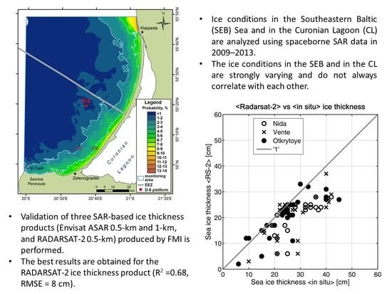
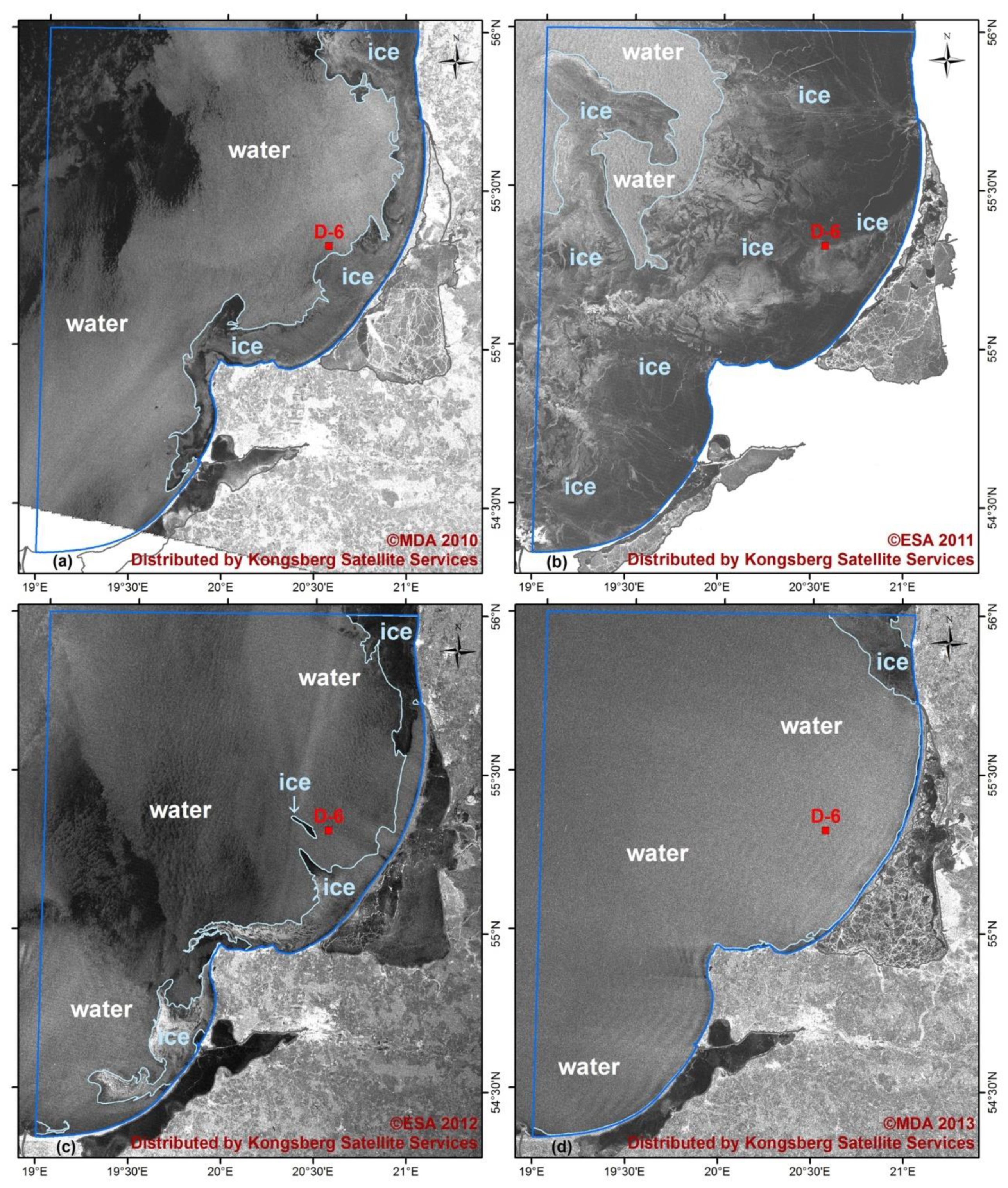
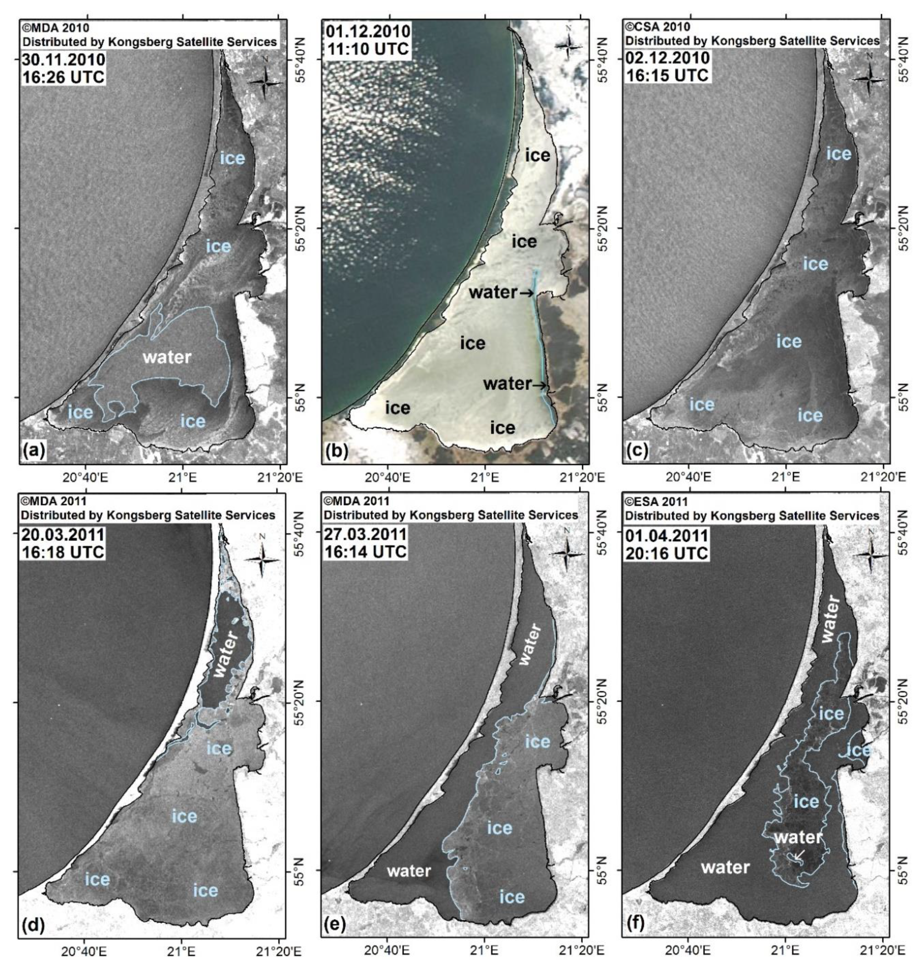
4.1. Ice Conditions in 2009–2013

Analysis of SAR data for the Southeastern Baltic Sea and the Curonian Lagoon shows that their ice regime is strongly varying from year to year. Figure 2 illustrates a very strong difference in the area covered by sea ice during the maximum ice cover development stage in the SEB in 2009–2013. In 2010 and 2012, the ice cover is observed along the coasts with a mean width of the ice band of about 5–15 km (Figure 2a,c). To the contrary, the ice extent is anomalously wide in February 2011 when it spreads up to 100 km offshore and covers about 90% of the marine part of the study area (Figure 2b). In 2013, the minimal spatial ice extent was recorded along the SEB with sea ice primarily observed along the Curonian Spit shore and north of the Port of Klaipėda (Figure 2d). Notably, the Curonian Lagoon was almost fully ice-covered during all these winter seasons.
The marine part of the study area is characterized by sporadic sea ice growth that clearly depends on wind conditions and air temperature. In contrast, the ice formation is more continuous and less sporadic in the Curonian Lagoon where it usually lasts from the first frosts in December–January till the end of winter season in March–April. Nevertheless, some winters were characterized by several freezing and melting periods in the CL. As already shown in [3], the northernmost part of the lagoon near the Port of Klaipėda often remains partially ice-free due to inflow of relatively warm and saline water from the Baltic Sea through the Klaipėda Strait and intensive shipping (Figure 3a,b). During severe winters, ships break the first ice forms and prevent the formation of stable ice cover in this area. Most often the marine water penetrates into the northern part of the lagoon through the Klaipėda Strait up to 25 km, and under particular meteorological conditions and strong westerly and north-westerly winds it may penetrate up to 40–50 km down the lagoon [40].
The temporal variability of ice extent in the CL and the SEB during four winter seasons in 2009–2013 is shown in Figure 4, while a more detailed analysis of ice cover changes in relation to air temperature and wind conditions is presented below.
In 2009–2010 ice season in the Curonian Lagoon has started on 12 December 2009, i.e., 3 days after the air temperature (Ta) dropped below zero. A further increase of wind speed above 10 m/s has stimulated intensive water mixing and cooling of the shallow lagoon resulting in full freeze up dated on 19 December 2009. The coastal zone of the SEB was ice-free at that moment, while a thin strip of ice was later observed along the Curonian Spit on 22 December and disappeared on 24 December 2009, when the Ta became positive (Figure 4).
Following a week of negative Ta values, sea ice formation in the SEB started again on 8 January 2010. Despite moderate and strong winds observed in that period, the ice cover spread rather fast along the Curonian Spit coast. A continuous freezing period lasted until 18 February 2010, and the maximum ice extent over the SEB was recorded on 8 February 2010 covering about 16 % of the study area (see Figure 2a and Figure 4). Strong winds and the rise of Ta in the second half of February 2010 stimulated the ice break-up and rapid melting, resulting in almost ice-free conditions observed on 3 March 2010. A short period of negative Ta down to −6 °C during the next week leaded to a partial ice formation that completely decayed on 19 March 2010.
In the Curonian Lagoon, the ice cover was more stable (Figure 4). The melt onset started in the north-western part of the lagoon in the beginning of March 2010. A small fracture of open water near Pervalka was well seen both in Envisat ASAR and MODIS Aqua images acquired on 10–11 March 2010 (Figure 5), and not captured visually at Nida and Ventė stations located nearby. Under westerly winds and positive Ta the ice melt moved further north- and eastward until reaching the eastern CL coast. Further warming led to the ice break-up in the central part of the CL. The last observation of ice during this winter season was made on 8 April 2010 along the eastern CL coast. The total ice season duration in 2009–2010 was 115 days and 65 days for the CL and the SEB, respectively.
The ice season of 2010–2011 started in the CL in late November, when early frosts and strong winds above 15 m/s (Figure 4) led to a fast cooling and freezing of the lagoon well depicted in Figure 6a–c. RADARSAT-2 image acquired on 30 November 2010 shows an intensive ice cover formation that spans the entire northern and central parts of the lagoon, as well as the regions along the coast in the southern CL with open water observed only in its central part (Figure 6a). MODIS visible band image acquired on the next day, 1 December 2010, shows the lagoon already fully ice-covered (Figure 6b), confirmed by RADARSAT-1 image of 2 December 2010 (Figure 6c).
In the marine part, the ice cover started to form two weeks later along the northern coast of the Sambia Peninsula. Prior to 1 February 2011, sea ice was observed mainly under moderate winds and subzero temperatures in the form of grease ice drifting along the coast. From 10 February 2011, a rapid drop of Ta down to −15 °C led to an extensive ice formation reaching 15,725 km2 (about 87% of the marine study area) by 24 February 2011 (see Figure 2b and Figure 4). That was the maximum ice extent recorded in the SE Baltic during the study period. Ice melting started in the beginning of March, and on 7 March 2011, only grease ice was detected along the Lithuanian coast and the Vistula Spit. The last observation of ice was recorded on 15 March 2011. It total, sea ice in the SEB was observed during 68 days within six episodes of ice formation.
In the Curonian Lagoon, ice melt onset was dated on 10 March 2011 (Figure 4). The ice break-up started in the northern part of the lagoon (Figure 6d), and then spread along the entire western coast. Varying winds caused a strong ice accumulation on the coasts near Nida in some cases damaging the coastal infrastructure (Figure 3c,d). Later on, strong westerly winds of 10–15 m/s caused an ice drifting eastward (Figure 6e). The ice cover remained longest in the central CL close to Neman Delta (Figure 6f). The overall length of the melting season was more than 3 weeks, and complete ice decay was dated on 4 April 2011 with the ice season duration equal to 127 days.
The ice season of 2011–2012 was the shortest during the period of observations starting in second half of January 2012 both in the CL and in the SEB (Figure 4). A rapid drop of Ta within a week period down to −21 °C and moderate winds triggered a fast ice formation and full freezing of the CL dated on 6 February 2012 (Figure 4). Eight days later, the first ice forms also appeared along the SEB coast. The ice extent grew quite rapidly and peaked on 11 February 2012 covering about 12% of the marine study area (Figure 2c). However, the next week was characterized by a sharp increase in Ta and wind conditions that stimulated ice melting in the SEB and its full decay on 17 February. In the CL, the melt onset was dated on 3 March and the last observation of ice was recorded on 31 March 2012 along the northeastern coast of the CL. The ice season duration for the CL and the SEB were 71 and 23 days, respectively.
In winter season 2012–2013, strong winds above 15 m/s and negative air temperature contributed to the ice formation in the CL in mid-December 2012 (see Figure 4). An increase of Ta in the end of December and strong westerly winds led to the ice melt along the coast of CL. Later on, with the onset of frosts, the CL became completely ice-covered again (see Figure 4).
In the SEB, the ice season was characterized by four ice formation episodes. The first fast ice was observed along the shore of the Curonian Spit on 16 January 2013. The maximum ice cover development was recorded by RADARSAT-2 on 23 January 2013, covering only about 3.4% of the marine study area (see Figure 2d). However, just a week later the ice cover completely disappeared when the air temperature rose above zero. The last two ice formation episodes were rather short, only 5–6 days long, observed in mid- and late March 2013 (see Figure 4). During these episodes, the formation of fast ice was observed along the coast from Baltiysk to the northern part of the marine study area. The last detection of sea ice was made on 26 March 2013.
As usual, the ice melt in the Curonian Lagoon began in its northern part. On 2 March 2013, open water reached Juodkrantė in the northwestern part of the CL (see Figure 1 for details). Other ice-covered parts of the lagoon remained stable till the end of March 2013. In the beginning of April 2013, when Ta was stably above zero, ice melting started near Ventė and then expanded along the northeastern coast of the lagoon. Ice-free regions strongly increased southward towards the central part of the lagoon, as both SAR and MODIS data suggest (Figure 7). A strong air temperature rise above 5 °C observed after 12 April 2013 led to the fast ice melt along the southern coasts of the lagoon, where it remained longest till 15 April 2013 (see Figure 7). It total, the ice season duration for winter 2012–2013 counted for 24 days in the SE Baltic Sea and 130 days in the Curonian Lagoon.
Figure 8 shows a composite map of ice cover probability in the SE Baltic obtained during an extended period of 2004–2019 for February, the month of the maximum ice cover development in this region [14]. As seen, the ice cover is observed most frequently along the southwestern part of the Curonian Spit and north of Klaipėda Strait, where an intense outflow of ice floes from the CL is frequently observed during the ice season. In 5% of cases the ice extent covers about 5 km band adjacent to the coast. A wider ice cover extent is observed less frequently, yet, in some rare cases it might span almost the entire SEB, as in February 2011 (Figure 2b).
Figure 9 shows spatial maps of ice cover probability in the Curonian Lagoon during 2009–2013. One common feature that is seen during all winter seasons is the highest ice cover probability (i.e., longest ice cover season) in the southeastern part of the lagoon. Depending on background air temperature and wind conditions, the area of longest ice observations (brown color in Figure 8) could be very large (25 km wide) covering almost the entire central and southern parts of the lagoon as in 2010–2011, rather narrow (5–8 km wide) as in 2011–2012, or have inhomogeneous pattern as in 2009–2010 and 2012–2013. The shortest ice season is clearly observed in the northern part of the lagoon, in agreement with [3]. Here, the location and area of minimal ice cover regions differ from year to year and are mainly determined by the wind conditions (Figure 9). Under prevalence of westerly-northwesterly winds, the sea water from the SEB enters the lagoon and together with mechanical wind action trigger the ice break up along the northwestern CL coast and its drift and accumulation along the opposite northeastern coast (Figure 9b,c). The higher is the wind action, the larger is the area of minimal ice cover in the northern lagoon part (compare Figure 9a–c). When the easterly and southeasterly winds dominate, the region of lowest ice frequency spans the entire northern part including the northeastern CL coast down to the northern Neman Delta (Figure 9d).

4.2. Validation of SAR-Based Ice Thickness Products

As already mentioned before, ice thickness (IT) measurements in the Curonian Lagoon were performed only at several coastal stations and, therefore, lack the spatial details of IT distribution over the entire lagoon. In turn, satellite observations provide a unique possibility to derive spatially detailed ice thickness maps for the large ice-covered regions of the Baltic Sea [41]. In this subsection we aim to explore the quality of SAR-based IT retrievals over the Curonian Lagoon through the comparison of satellite-based IT products with in-situ ice thickness measurements. Since the latter were only available till the winter of 2012–2013 and satellite products became available from 2010–onwards, our analysis is limited to three winter seasons of 2010–2013. In winter 2010–2011, we consider two types of ASAR-based ice thickness data (ASAR 0.5-km and ASAR 1-km), while in 2011–2012 ASAR 0.5-km and RADARSAT-2 (RS-2) 0.5-km products are used. Due to failure of Envisat ASAR in April 2012, we consider only the RS-2 0.5-km product for the winter 2012–2013.
As seen from Figure 10a, the ASAR-based ice thickness values nicely follow the gradual ice thickness rise from 5 cm to 25 cm observed in the beginning of winter 2010–2011 at Nida and Ventė, with some overestimates at Otkrytoye station. The discrepancy between the two data sources grows when the true ice thickness experiences a step-like rise till around 40 cm in the middle of the season around 27 January–26 February 2011. After that, the SAR-based estimates grow up and start to reproduce the observed IT levels at all stations with the ASAR 1-km IT product performing somewhat better, while the 0.5-km IT product showed a better performance during the first half of the season.
In winter 2011–2012, the ice thickness is gradually rising and peaks at 40–42 cm around 21–23 February 2012 (Figure 10b). During this winter season, both the RS-2 and the ASAR products show rather similar results and, in general, reproduce the observed seasonal changes of IT values. Nevertheless, satellite products largely underestimate the observed IT values by 10–15 cm. One may see a clear delay of about 7–10 days between the in-situ and the satellite IT curves. In satellite data, the 40-cm ice thickness level is reached only in the end of February 2012, after which the gap between the satellite and the in-situ data is almost negligible. The smallest difference is observed for Otkrytoye station in the southern CL part where the ice conditions are more stable (Figure 9c).
The winter season of 2012–2013 is characterized by relatively low ice thickness values generally not exceeding 20–30 cm throughout the season (Figure 10c). The performance of the RS-2 product is rather adequate, it correlates quite well with the observed ice thickness values with only some minor underestimates for Ventė and Otkrytoye stations. The correlation for Nida station is also good apart of two short-term episodes of rapid ice thickness growth observed after 15 February 2013.
Figure 11 shows two scatter plots where the in-situ ice thickness measurements are plotted against the satellite products separately for Envisat ASAR and RS-2. The corresponding statistical measures describing the overall performance of the three different SAR-based IT products are given in Table 2. The comparison between the ASAR 0.5-km and 1-km products shows that the 0.5-km product performs slightly better with a mean R2 equal to 0.64 (Table 2). For this reason, only the ASAR 0.5-km product values are plotted in Figure 11a. As seen from Figure 11a and Table 2, the best results are obtained for Ventė station where R2 is equal to 0.81 and a root mean square error (RMSE) is smallest, 9.7 cm. The plausible explanation of this fact could be a more stable ice cover conditions near Ventė (for example, see Figure 9b,c). The largest RMSE is obtained for Nida station (14.1 cm), while the lowest R2 is obtained for Otkrytoye station where the ASAR product both over- and underestimates the observed ice thickness values.
In contrast to the ASAR performance, the RS-2 ice thickness values have much smaller spread around 1:1 line (Figure 11b) with RMSE in the range of 6.7–9 cm (Table 2). Moreover, RS-2 data are found to predominantly underestimate the observed ice thickness levels at all stations unlike the ASAR product that partly overestimates the observations. The best performance is obtained for Otkrytoye station with R2 equal to 0.78 and smallest RMSE value (6.7 cm). The correlation of RS-2 data with in-situ measurements at Ventė station is R2 = 0.65 but is characterized by the relatively high RMSE (around 9 cm).

5. Discussion

The Baltic Sea is a vital waterway connecting densely populated and highly industrialized countries of Northern Europe, and the Port of Klaipėda is one of the busiest in the SE Baltic Sea. Shipping operations in the Port of Klaipėda, as well as navigation and fisheries in the Curonian Lagoon in wintertime depend on accurate now- and forecasting of local weather and ice conditions. Many numerical forecasting models suffer from a lack of calibration data because relevant ice cover properties such as ice extent, concentration, thickness, drift and deformation are difficult and expensive to monitor [41]. In turn, the accurate knowledge of ice conditions obtained from satellite data leads to a more adequate modeling of hydrodynamic processes and circulation patterns in the Curonian Lagoon [42].
In this work we use visual interpretation and manual digitization of SAR data to retrieve ice cover extent in the SE Baltic Sea and the Curonian Lagoon. While the human supervised method could have various biases in defining the area of ice-covered regions, it is widely used by ice analysts to produce ice charts at FMI (Finland), Swedish Meteorological and Hydrological Institute (Sweden), Arctic and Antarctic Research Institute (Russia), etc. In our case, the main advantage of the method is the ability to preserve the initial high resolution of SAR data at 50–150 m spatial resolution that is critical to study the ice conditions over small coastal areas and semi-enclosed water bodies. Nevertheless, we must acknowledge that more elaborated and fully automated methods of sea ice parameter retrieval from SAR data exist [17,18,19,20,21,28].
We have also attempted to evaluate the quality of several SAR-based IT products produced by FMI and distributed by CMEMS, in the shallow semi-enclosed Curonian Lagoon where the number of in-situ ice thickness measurements is small. To our knowledge, there has been only a limited validation of these FMI IT products versus in-situ IT measurements made from the Finnish ice breakers in the northern Baltic Sea counting only for 27 match-ups in total [22]. In particular, the validation results showed rather large scatter and mismatch up to 50 cm between the SAR-based IT product and in-situ IT measurements for the range of observed IT values of 10–65 cm [22]. In our case, the largest difference between the ASAR 0.5-km IT product and in-situ IT measurements was 34 cm, while for the RS-2 0.5-km IT product it was even less, 22 cm, for the range of observed IT values of 4–55 cm. In this sense, our validation study based on a larger number of match-up points suggests that the considered SAR-based IT products perform better in the shallow Curonian Lagoon than in the northern Baltic Sea.
Some information is also available on the performance of FMI multi-sensor IT product for the Barents and Kara Seas. This product is slightly different from the one used in our study. It is based on merging ice thickness derived from AMSR2 radiometer data, TOPAZ-4 coupled ocean-sea ice model and SAR (see details in [43]). The validation of this multi-sensor 1-km IT product based on RADARSAT-2 data versus in-situ IT measurements derived from ship-mounted electromagnetic induction instrument EM31 was done in March 2014 east of Svalbard [44]. The results based on 2758 match-up points showed good accuracy in identification of thin ice class (<30 cm). Only in 10% of cases the multi-sensor IT product underestimated the observed IT values above 30 cm and showed thin ice class (<30 cm) [44]. In our case, the three considered FMI IT products showed thin ice class and underestimated the observed IT values above 30 cm in 30% of cases, suggesting that multi-sensor IT product enriched with model data performs better at least for IT values above 30 cm. However, most of our results and those from the Arctic region were obtained for thin ice class. Yet, the detailed statistics of multi-sensor IT product performance for thin ice class in the Arctic is not available and, hence, we can’t make any solid conclusions on the quality of FMI IT products in the Curonian Lagoon in comparison to the results obtained in the Arctic.
We should also note that the contemporary version of the FMI IT product for the Baltic Sea is largely based on Sentinel-1 data (in combination with RADARSAT-2, [39]) that were not considered in this study. Availability of data from two SAR sensors carried by Sentinel-1A and -1B suggests a higher frequency of SAR observations over our study site [3] and a better potential for future validation activities, provided the number of regular in-situ IT measurements would increase.
Lastly, L-band SAR data from ALOS-2 PALSAR-2 were recently shown to have better results than conventional C-band SAR data in defining key sea ice parameters in the Arctic Ocean, including ice thickness [45]. As such, they could be also used in regular sea ice monitoring to complement the data available from operational C-band and X-band instruments for the Baltic Sea and better the quality of existing sea ice products.

6. Conclusions

Here we show that a combination of spaceborne SAR and optical imagery with in-situ data from local hydrometeorological stations can significantly improve our knowledge about the ice regime in the seasonally ice-covered regions like the Southeastern Baltic Sea and the Curonian Lagoon.
As shown, the ice conditions in the SEB and in the CL are strongly varying from year to year. In the SEB, the ice cover could be observed either only along the coast within 5–15 km band covering only about 3–4% of the study area (January 2013), or spread up to 100 km offshore and cover almost the entire SEB, as in February 2011. In turn, the Curonian Lagoon is almost fully ice-covered during all considered winters apart of its northern part that is subject to sea water inflow and various port activities. The SEB is also characterized by sporadic sea ice growth that may appear and decay several times per season (e.g., 6 episodes in 2010–2011) depending on background weather conditions. In contrast, the ice cover is more stable in the Curonian Lagoon where it usually lasts from the first frosts till the end of winter season. Nevertheless, it also possesses multiple periods of partial melting and re-freezing that becomes more frequent during the last decades.
The dates of maximal ice extent in the SEB range from the end of January till the end of February. The mean ice season duration here is equal to 45 days ranging from 23 days in 2011–2012 to 68 days in 2010–2011. The ice season of 2011–2012 was the shortest during 2009–2013 both for the SEB and the CL, lasting for 23 and 71 days, respectively. However, the ice season duration in the sea and in the lagoon do not always correlate with each other. For example, in 2012–2013 it counted only for 24 days in the SEB (second lowest value) versus the longest ice season duration of 129 days in the lagoon.
In the Curonian Lagoon, the rapid ice cover formation is often stimulated by the high winds above 10–15 m/s that intensify water mixing and cooling of the shallow brackish lagoon. The ice break-up usually starts in its northern part [3] and could be associated with an intense ice drift sometimes followed by heavy ice accumulation on the coasts under high winds. The highest ice cover frequency (i.e., longest ice cover season) is observed in the southeastern part of the lagoon, while the lowest one is clearly seen in its northern part. Here, the location and area of regions with the shortest ice season differs from year to year and is mainly determined by the wind conditions. Under prevalence of westerly-northwesterly winds, the sea water enters the lagoon and together with the mechanical wind action trigger the ice break up along the north-western CL coast. When the easterly and southeasterly winds dominate, the region of lowest ice cover frequency spans the entire northern part including the northeastern CL coast down to the northern Neman Delta.
The comparison and validation of three SAR-based ice thickness products (ASAR 0.5-km, ASAR 1-km and RADARSAT-2 0.5-km) versus in-situ measurements has shown very promising results. All satellite products perform rather well for the periods of gradual ice thickness growth. During the episodes of the rapid ice thickness increase, all products underestimate the ice thickness by 10–20 cm (20–50%) reaching the observed level after about a month period. During such periods, the observed difference could be compensated by simply adding on average 15 cm to the SAR-based ice thickness values. The best results are obtained for the RADARSAT-2 0.5-km ice thickness product, it has the highest station-mean R2 value (0.68) and the lowest mean RMSE (around 8 cm), followed by the ASAR 0.5-km product.
The overall performance of satellite products is better near Ventė and Otkrytoye stations where the ice conditions are more stable, while the largest RMSE and the lowest R2 values are obtained for Nida station characterized by more dynamic ice cover conditions. All in all, the validation results show that the SAR-based ice thickness products provide rather adequate ice thickness estimates for the shallow brackish coastal lagoon. Though our comparison spans only several winter seasons and doesn’t consider ice thickness products from other contemporary SAR missions (e.g., Sentinel-1), we believe that, upon careful validation, such products can provide useful information for spatial and temporal analysis of ice thickness variations in coastal waters and semi-enclosed shallow water bodies where the number of field observations is insufficient or lacking.

Author Contributions

Conceptualization, I.E.K., E.V.K. and A.G.K.; methodology, E.V.K. and I.E.K.; software, E.V.K. and I.E.K.; validation, I.E.K. and I.D.; formal analysis, I.E.K. and E.V.K.; investigation, all authors; data curation, E.V.K. and I.E.K.; writing—original draft preparation, I.E.K., E.V.K., A.G.K.; writing—review and editing, I.D., A.G.K.; visualization, E.V.K., I.E.K., I.D.; supervision, I.E.K.; funding acquisition, I.E.K. and E.V.K. All authors have read and agreed to the published version of the manuscript.

Funding

This research and the APC was funded by the Russian Science Foundation, grant no. 17-77-30019. Collection of satellite data was funded by the state assignment of IO RAS, theme no. 0149-2019-0013. Study of spatial sea ice extent variability was funded by the Russian Foundation for Basic Research, grant no. 19-45-390012.

Acknowledgments

The authors would like to thank LUKOIL-KMN, Ltd. (Kaliningrad, Russia) for providing satellite radar imagery for the Southeastern Baltic Sea, and the Marine Research Department of the Environment Protection Agency of Lithuania for providing the hydrometeorological and the ice thickness data from coastal stations.

Conflicts of Interest

The authors declare no conflict of interest.

References

  1. Granskog, M.; Kaartokallio, H.; Kuosa, H.; Thomas, D.N.; Vainio, J. Sea ice in the Baltic Sea—A review. Estuar. Coast. Shelf Sci. 2006, 70, 145–160. [Google Scholar] [CrossRef]
  2. Chubarenko, B.; Chechko, V.; Kileso, A.; Krek, E.; Topchaya, V. Hydrological and sedimentation conditions in a non-tidal lagoon during ice coverage—The example of Vistula Lagoon in the Baltic Sea. Estuar. Coast. Shelf Sci. 2019, 216, 38–53. [Google Scholar] [CrossRef]
  3. Idzelytė, R.; Kozlov, I.E.; Umgiesser, G. Remote sensing of ice phenology and dynamics of Europe’s largest coastal lagoon (The Curonian Lagoon). Remote Sens. 2019, 11, 2059. [Google Scholar] [CrossRef] [Green Version]
  4. Eremina, T.R.; Bugrov, L.Y.; Maksimov, A.A.; Ryabchenko, V.A.; Shilin, M.B. The Baltic Sea. In Second Assessment Report of Roshydromet on Climate Change and Its Concequences on Territory of Russian Federation; Kattsov, V.M., Semenov, S.M., Eds.; Institute of Global Climate and Ecology: Moscow, Russia, 2014; pp. 615–643. (In Russian) [Google Scholar]
  5. Dailidienė, I.; Baudler, H.; Chubarenko, B.; Navrotskaya, S. Long term water level and surface temperature changes in the lagoons of the southern and eastern Baltic. Oceanologia 2011, 53, 293–308. [Google Scholar] [CrossRef] [Green Version]
  6. Omstedt, A.; Elken, J.; Lehmann, A.; Leppäranta, M.; Meier, H.E.M.; Myrberg, K.; Rutgersson, A. Progress in physical oceanography of the Baltic Sea during the 2003–2014 period. Prog. Oceanogr. 2014, 128, 139–171. [Google Scholar] [CrossRef]
  7. Serykh, I.V.; Kostianoy, A.G. About the climatic changes in the temperature of the Baltic Sea. Fundam. Prikl. Gidrofiz. 2019, 12, 5–12. [Google Scholar]
  8. Helsinki Commission (HELCOM). Climate Change in the Baltic Sea Area: HELCOM Thematic Assessment in 2013; Baltic Sea Environment Proceedings No. 137; Helsinki Commission: Helsinki, Finland, 2013; 66p. [Google Scholar]
  9. Elken, J.; Lehmann, A.; Myrberg, K. Recent changes in Baltic Sea oceanographic conditions, with some effects to the ecosystem status. In Proceedings of the 10th Baltic Sea Science Congress, Riga, Latvia, 15–19 June 2015; p. 34. [Google Scholar]
  10. Haapala, J.; Ronkainen, L.; Schmelzer, N.; Sztobryn, M. Recent change—Sea ice. In Second Assessment of Climate Change for the Baltic Sea Basin; The BACC Author Team, Ed.; Springer: Cham, Switzerland, 2008; pp. 145–153. [Google Scholar]
  11. Von Storch, H.; Barkhordarian, A. Detection and attribution of climate change in the Baltic Sea Region. In Proceedings of the 10th Baltic Sea Science Congress, Riga, Latvia, 15–19 June 2015; p. 8. [Google Scholar]
  12. Dailidienė, I.; Davulienė, L.; Kelpšaitė, L.; Razinkovas, A. Analysis of the climate change in Lithuanian coastal areas of the Baltic Sea. J. Coast. Res. 2012, 28, 557–569. [Google Scholar] [CrossRef]
  13. Kļaviņš, M.; Avotniece, Z.; Rodinovs, V. Dynamics and impacting factors of ice regimes in Latvia inland and coastal waters. Proc. Latv. Acad. Sci. 2016, 70, 400–408. [Google Scholar] [CrossRef] [Green Version]
  14. Krek, E.V.; Stont, Z.I.; Bukanova, T.V. Ice conditions in the Southeastern Baltic Sea from satellite data (2004–2019). J. Ocean Res. 2020, 48, 18–33. (In Russian) [Google Scholar] [CrossRef]
  15. Dailidienė, I. Kuršių marių hidrologinio režimo pokyčiai. Geografija 2007, 43, 36–43. [Google Scholar]
  16. Bagdanavičiūtė, I.; Umgiesser, G.; Vaičiūtė, D.; Bresciani, M.; Kozlov, I.; Zaiko, A. GIS-based multi-criteria site selection for zebra mussel cultivation: Addressing end-of-pipe remediation of a eutrophic coastal lagoon ecosystem. Sci. Total Environ. 2018, 634, 990–1003. [Google Scholar] [CrossRef] [PubMed]
  17. Karvonen, J.; Simila, M.; Heiler, I. Ice thickness estimation using SAR data and ice thickness history. In Proceedings of the IEEE International Geoscience and Remote Sensing Symposium 2003 (IGARSS 03), Toulouse, France, 21–25 July 2003; Volume 1, pp. 74–76. [Google Scholar]
  18. Similä, M.; Karvonen, J.; Haas, C. Inferring the degree of ice field deformation in the Baltic Sea using Envisat ASAR images. In Advances in SAR Oceanography from Envisat and ERS Missions, Proceedings of the SEASAR 2006, Frascati, Italy, 23–26 January 2006; Lacoste, H., Ouwehand, L., Eds.; ESA Publications Division, ESTEC: Noordwijk, The Netherlands, 2006. [Google Scholar]
  19. Askne, J.; Dierking, W. Sea ice monitoring in the Arctic and Baltic Sea using SAR. In Remote Sensing of the European Seas; Barale, V., Gade, M., Eds.; Springer: Dordrecht, The Netherlands, 2008; pp. 383–398. [Google Scholar] [CrossRef]
  20. Karvonen, J. Operational SAR-based sea ice drift monitoring over the Baltic Sea. Ocean Sci. 2012, 8, 473–483. [Google Scholar] [CrossRef] [Green Version]
  21. Karvonen, J. Evaluation of the operational SAR based Baltic Sea ice concentration products. Adv. Space Res. 2015, 56, 119–132. [Google Scholar] [CrossRef]
  22. Eastwood, S.; Karvonen, J.; Dinessen, F.; Fleming, A.; Pedersen, L.T.; Saldo, R.; Buus-Hinkler, J.; Hackett, B.; Ardhuin, F.; Kreiner, M.B.; et al. Quality Information Document for SI TAC Sea Ice Products; EU Copernicus Marine Service, 2020; Issue 2.9; 71p, Available online: https://cmems-resources.cls.fr/documents/QUID/CMEMS-OSI-QUID-011-001to007-009to012.pdf (accessed on 6 October 2020).
  23. Žaromskis, R. Oceans, Seas, Estuaries; Debesija: Vilnius, Lithuania, 1996. (In Lithuanian) [Google Scholar]
  24. Gasiūnaitė, Z.R.; Daunys, D.; Olenin, S.; Razinkovas, A. The Curonian Lagoon. In Ecology of Baltic Coastal Waters; Schiewer, U., Ed.; Springer: Berlin/Heidelberg, Germany, 2008; pp. 197–215. [Google Scholar] [CrossRef]
  25. Dailidienė, I.; Davulienė, L. Salinity trend and variation in the Baltic Sea near the Lithuanian coast and in the Curonian Lagoon in 1984–2005. J. Mar. Syst. 2008, 74, 20–29. [Google Scholar] [CrossRef]
  26. Onstott, R.G.; Shuchman, R.A. SAR measurements of sea ice. In Synthetic Aperture Radar Marine User’s Manual; Jackson, C.R., Apel, J.R., Eds.; U.S. Department of Commerce: Washington, DC, USA, 2004; pp. 81–115. [Google Scholar]
  27. Johannessen, O.M.; Alexandrov, V.Y.; Frolov, I.Y.; Bobylev, L.P.; Sandven, S.; Pettersson, L.H.; Kloster, K.; Babich, N.G.; Mironov, Y.U.; Smirnov, V.G. Remote Sensing of Sea Ice in the Northern Sea Route: Studies and Applications; Springer: Chichester, UK, 2007. [Google Scholar]
  28. Dierking, W. Sea ice monitoring by synthetic aperture radar. Oceanography 2013, 26, 100–111. [Google Scholar] [CrossRef]
  29. Muckenhuber, S.; Nilsen, F.; Korosov, A.; Sandven, S. Sea ice cover in Isfjorden and Hornsund, Svalbard (2000–2014) from remote sensing data. Cryosphere 2016, 10, 149–158. [Google Scholar] [CrossRef] [Green Version]
  30. Kozlov, I.; Dailidienė, I.; Korosov, A.; Klemas, V.; Mingėlaitė, T. MODIS-based sea surface temperature of the Baltic Sea Curonian Lagoon. J. Mar. Syst. 2014, 129, 157–165. [Google Scholar] [CrossRef]
  31. Dabuleviciene, T.; Kozlov, I.E.; Vaiciute, D.; Dailidiene, I. Remote sensing of coastal upwelling in the South-Eastern Baltic Sea: Statistical properties and implications for the coastal environment. Remote Sens. 2018, 10, 1752. [Google Scholar] [CrossRef] [Green Version]
  32. Karimova, S.S.; Gade, M. Improved statistics of sub-mesoscale eddies in the Baltic Sea retrieved from SAR imagery. Int. J. Rem. Sens. 2016, 37, 2394–2414. [Google Scholar] [CrossRef]
  33. Ginzburg, A.I.; Krek, E.V.; Kostianoy, A.G.; Solovyev, D.M. Evolution of mesoscale anticyclonic vortex and vortex dipoles/multipoles on its base in the South-Eastern Baltic (satellite information: May–July 2015). J. Ocean Res. 2017, 45, 10–22. (In Russian) [Google Scholar] [CrossRef] [Green Version]
  34. Ginzburg, A.I.; Krek, E.V.; Kostianoy, A.G.; Solovyev, D.M. On the role of mesoscale vortices in the oil spill transport in the Southeastern Baltic Sea (satellite information). J. Ocean Res. 2019, 47, 8–19. (In Russian) [Google Scholar] [CrossRef]
  35. Kozlov, I.E.; Kudryavtsev, V.N.; Johannessen, J.A.; Chapron, B.; Dailidienė, I.; Myasoedov, A.G. ASAR imaging for coastal upwelling in the Baltic Sea. Adv. Space Res. 2012, 50, 1125–1137. [Google Scholar] [CrossRef]
  36. Kozlov, I.E.; Artamonova, A.V.; Manucharyan, G.E.; Kubryakov, A.A. Eddies in the Western Arctic Ocean from spaceborne SAR observations over open ocean and marginal ice zones. J. Geophys. Res. Oceans 2019, 124, 6601–6616. [Google Scholar] [CrossRef] [Green Version]
  37. Kozlov, I.E.; Plotnikov, E.V.; Manucharyan, G.E. Brief Communication: Mesoscale and submesoscale dynamics of marginal ice zone from sequential SAR observations. Cryosphere 2020, 14, 2941–2947. [Google Scholar] [CrossRef]
  38. Stont, Z.; Bulycheva, E.; Bukanova, T. Ice conditions in the South-Eastern Baltic by satellite data and field observations in 2006–2013. In Proceedings of the Baltic Sea Science Congress, Klaipėda, Lithuania, 26–30 August 2013; p. 251. [Google Scholar]
  39. Karvonen, J.; Heiler, I.; Seinä, A.; Hackett, B. Product User Manual for Baltic Sea Ice Products SEAICE_BAL_SEAICE_L4_NRT_OBSERVATIONS_011_004/011; EU Copernicus Marine Service, 2018; Issue 2.7; 28p, Available online: https://resources.marine.copernicus.eu/documents/PUM/CMEMS-OSI-PUM-010-016.pdf (accessed on 6 October 2020).
  40. Zemlys, P.; Ferrarin, C.; Umgiesser, G.; Gulbinskas, S.; Bellafiore, D. Investigation of saline water intrusions into the Curonian Lagoon (Lithuania) and two-layer flow in the Klaipėda Strait using finite element hydrodynamic model. Ocean Sci. 2013, 9, 573–584. [Google Scholar] [CrossRef] [Green Version]
  41. Löptien, U.; Axell, L. Ice and AIS: Ship speed data and sea ice forecasts in the Baltic Sea. Cryosphere 2014, 8, 2409–2418. [Google Scholar] [CrossRef] [Green Version]
  42. Idzelytė, R.; Mėžinė, J.; Zemlys, P.; Umgiesser, G. Study of ice cover impact on hydrodynamic processes in the Curonian Lagoon through numerical modeling. Oceanologia 2020. [Google Scholar] [CrossRef]
  43. Similä, M.; Mäkynen, M.; Cheng, B.; Rinne, E. Multisensor data and thermodynamic sea-ice model based sea-ice thickness chart with application to the Kara Sea, Arctic Russia. Ann. Glaciol. 2013, 54, 241–252. [Google Scholar] [CrossRef] [Green Version]
  44. Melsheimer, C.; Mäkynen, M.; Rasmussen, T.; Rudjord, Ø.; Simila, M.; Sohlberg, R.; Walker, N. Comparison and validation of four Arctic sea ice thickness products of the EC POLAR ICE project. In Proceedings of the ESA Living Planet Symposium 2016, Prague, Czech Republic, 9–13 May 2016; Volume 740, p. 8. [Google Scholar]
  45. Karvonen, J.; Rinne, E.; Sallila, H.; Mäkynen, M. On suitability of ALOS-2/PALSAR-2 dual-polarized SAR data for Arctic sea ice parameter estimation. IEEE Trans. Geosci. Rem. Sens. 2020, 58, 7969–7981. [Google Scholar] [CrossRef]
Figure 1. Map of the study area. Legend: 1—marine part of the study area; 2—the Curonian Lagoon; 3—boundaries of exclusive economic zones (EEZ); 4—ice monitoring stations in the Curonian Lagoon; 5—D-6 oil platform. The contour lines show isobaths.
Remotesensing 12 03754 g001
Figure 2. Maximum sea ice extent in the Southeastern Baltic Sea in winter seasons of 2009–2013 observed in spaceborne SAR data: (a) RADARSAT-2 on 8 February 2010 (05:05 UTC); (b) Envisat ASAR on 24 February 2011 (09:13 UTC); (c) Envisat ASAR on 11 February 2012 (09:10 UTC); (d) RADARSAT-2 on 23 January 2013 (05:05 UTC). Light blue contours mark the boundaries between the open water and the ice-covered regions.
Remotesensing 12 03754 g002
Figure 3. Photographs illustrating the ice conditions in the Klaipėda Strait taken on: (a) 3 January 2010 and (b) 13 February 2011; and (c,d) heavy ice accumulation along the coasts of Nida on 17 March 2011. Photographs taken by I. Dailidienė and I. Kairytė.
Remotesensing 12 03754 g003
Figure 4. Variability of ice extent in the Curonian Lagoon (left column) and in the Southeastern Baltic Sea (right column) obtained from satellite data for winters of 2009–2013. Legend: 1—percentage of the ice extent within the study area; 2—daily average air temperature (Ta); 3—daily average wind speed. Zero values in both diagrams mean absence of ice cover.
Remotesensing 12 03754 g004
Figure 5. Start of ice break-up in the Curonian Lagoon as seen in (a) Envisat ASAR image acquired on 10 March 2010; (b) MODIS Aqua visible-band image acquired on 11 March 2010.
Remotesensing 12 03754 g005
Figure 6. Ice formation and decay in the Curonian Lagoon during winter 2010–2011 as observed in: (a) RADARSAT-2 image of 30 November 2010 (16:26 UTC); (b) MODIS Aqua image of 1 December 2010; (c) RADARSAT-1 image of 2 December 2010 (16:15 UTC); (d) RADARSAT-2 image of 20 March 2011 (16:18 UTC); (e) RADARSAT-2 image of 27 March 2011 (16:14 UTC); (f) Envisat ASAR image of 1 April 2011 (20:16 UTC). Light blue contours mark the boundaries between the open water and the ice-covered regions.
Remotesensing 12 03754 g006
Figure 7. Ice break-up and decay in the Curonian Lagoon in March–April 2013. Light blue contours mark the boundaries between the open water and the ice-covered regions.
Remotesensing 12 03754 g007
Figure 8. Probability of ice cover observations (%) in the SE Baltic near the Curonian Spit in February according to spaceborne SAR data during an extended period of 2004–2019 [14]. Light blue contours show isolines of 2% and 5% probabilities of ice cover observations.
Remotesensing 12 03754 g008
Figure 9. Probability of ice cover observations (%) in the Curonian Lagoon according to spaceborne SAR data in: (a) 2009–2010; (b) 2010–2011; (c) 2011–2012; (d) 2012–2013. Inserts show wind roses for the period from 20 November to 15 April.
Remotesensing 12 03754 g009
Figure 10. Comparison of Envisat ASAR and RADARSAT-2 ice thickness products with in-situ measurements for winter seasons of 2010–2013 for (a) Envisat ASAR 0.5-km and 1-km products in 2010–2011, (b) Envisat ASAR 0.5-km and RADARSAT-2 0.5-km products in 2011–2012, (c) RADARSAT-2 0.5-km in 2012–2013.
Remotesensing 12 03754 g010
Figure 11. Scatter plots of in-situ ice thickness measurements made at Nida, Ventė and Otkrytoye stations versus (a) Envisat ASAR 0.5-km and (b) RADARSAT-2 0.5-km ice thickness products.
Remotesensing 12 03754 g011
Table 1. Main characteristics of spaceborne SAR images used in the study.
SatelliteBandScene Size, kmSpatial Resolution, mNumber of ImagesPeriod
Envisat ASARC400 × 400150 × 150144November 2009–April 2012
RADARSAT-1C300 × 30050 × 5063December 2009–March 2013
RADARSAT-2C500 × 500100 × 10070December 2009–April 2013
Table 2. Statistical measures for SAR-derived ice thickness products as compared against in-situ measurements in the Curonian Lagoon.
StationASAR 1-kmASAR 0.5-kmRS-2 0.5-km
NRRMSE, cmNRRMSE, cmNRRMSE, cm
Nida370.5514.9460.6114.1350.588.8
Ventė390.818.6460.819.7330.659
Otkrytoye400.5713.5470.5913410.786.7
All1160.5912.61390.6412.41090.688.1
Publisher’s Note: MDPI stays neutral with regard to jurisdictional claims in published maps and institutional affiliations.

